learning about the interdependence between the macroeconomy

LEARNING ABOUT THE INTERDEPENDENCE BETWEEN THEMACROECONOMY AND THE STOCK MARKET

FABIO MILANI

University of California, Irvine

Abstract. How strong is the interdependence between the macroeconomy and the stockmarket?

This paper estimates a New Keynesian general equilibrium model, which includes a wealtheffect from asset price fluctuations to consumption, to assess the quantitative importance ofinteractions among the stock market, macroeconomic variables, and monetary policy.

The paper relaxes the assumption of rational expectations and assumes that economicagents learn over time and form near-rational expectations from their perceived model of theeconomy. The stock market, therefore, affects the economy through two channels: through atraditional “wealth effect” and through its impact on agents’ expectations. Monetary policydecisions also affect and are potentially affected by the stock market.

The empirical results show that the direct wealth effect is modest, but asset price fluctu-ations have had important effects on output expectations. Shocks in the stock market canaccount for a large portion of output fluctuations. The effect on expectations, however, hasdeclined over time.

Keywords: Stock Market, Wealth Channel, Monetary Policy, Constant-Gain Learning, BayesianEstimation, Expectations.

JEL classification: E32, E44, E52, E58.

Date: May 15, 2008.I would like to thank Efrem Castelnuovo for a very useful discussion and for comments, seminar participantsat UC Irvine and at the Society for Nonlinear Dynamics and Econometrics 2008 conference in San Franciscofor comments. Huy Pham provided excellent research assistance.Address for correspondence: Department of Economics, 3151 Social Science Plaza, University of California,Irvine, CA 92697-5100. Phone: 949-824-4519. Fax: 949-824-2182. E-mail: [email protected]. Homepage:http://www.socsci.uci.edu/˜fmilani.

LEARNING, THE MACROECONOMY, AND THE STOCK MARKET 1

1. Introduction

How strong are the links between the macroeconomy and the stock market?

The New Keynesian models that are widely employed to characterize the dynamics of

output and inflation and to study monetary policy typically abstract from the stock market.

Asset prices, however, can influence the economy through a variety of channels. Policy

discussions often emphasize the impact that asset price fluctuations can have on consump-

tion spending decisions: this is the so-called “wealth effect”. Monetary policy makers may

consider actively responding to asset prices if the wealth channel is sizeable. But the size

of the effect is still controversial: although most regressions that have been estimated in

the literature show a positive and significant causal effect of wealth on consumption,1 recent

studies conclude that the effect is smaller than previously thought (Lettau and Ludvigson,

2004, Case, Quigley, and Shiller, 2005). Additionally, asset prices can affect real activity

trough other channels, such as through a Tobin’s Q effect on investment and through a

balance sheet/credit channel effect.2

Another central area of interdependence involves the link between asset prices and mon-

etary policy decisions. Researchers have been interested in understanding both whether

monetary policy responds to asset price fluctuations and how strongly the latter are affected

by policy shocks (e.g., Rigobon and Sack, 2003, 2004, Bernanke and Kuttner, 2005, Biørnland

and Leitemo, 2008) or other macroeconomic fundamentals (e.g., Chen et al., 1986).

This paper adopts a structural New Keynesian model, which will be estimated on U.S.

data, to infer the strength of the interdependence among macroeconomic variables, monetary

policy, and the stock market. The model, which is based on Nistico (2005)’s extension of

Blanchard (1985)’s overlapping generations framework, includes a wealth effect from asset

prices to consumption, whose magnitude depends on a structural parameter, which affects

the length of the households’ planning horizon. Current output is affected by expectations

of future output, real interest rates, and by current financial wealth, which is influenced by

swings in stock prices. Current stock values depend on their own expected future values, on

expectations about future real activity, and on the ex ante real interest rate.

1Research goes back to Ando and Modigliani (1963); Poterba (2000) and Davis and Palumbo (2001) arerecent surveys.

2This paper will focus on the wealth channel; the Tobin’s Q and balance sheet effects are, instead, omittedfrom the analysis.

2 FABIO MILANI

In modeling the expectations formation, the paper relaxes the traditional informational

assumptions imposed by rational expectations and it assumes that agents form subjective –

near-rational – expectations and that they attempt to learn the model parameters over time.

Some critics of the conventional wealth channel effect have argued that changes in stock

wealth mainly affect consumption through changes in expectations and consumer confidence,

but no direct wealth effect exists.3 This paper includes both effects: a direct wealth effect of

asset prices on consumption and output, and an effect of asset prices on future expectations.

The estimation tries to empirically disentangle the two effects.

The model is estimated using Bayesian methods on monthly U.S. data. The constant gain

coefficient is jointly estimated with the structural parameters of the economy, so that the

learning process can be extracted from the data, rather than arbitrarily imposed.

1.1. Results. The empirical evidence suggests a small direct wealth effect of stock prices

on output. Fluctuations in the stock market, however, affect economic agents’ expectations

of future real activity. The effect has considerably varied over the sample: in the first half,

economic agents believed changes in the stock market to have a strong effect on output,

while they revised their beliefs downward in the second part of the sample.

Through such effect on expectations, therefore, the stock market plays an important role

for macroeconomic variables. In the 1960s-1970s, up to 60-70% of fluctuations in the output

gap were explained by shocks that originated in the stock market; the stock market also

acted to amplify the transmission of monetary policy shocks. The importance of stock

market shocks has declined over the sample: in the 1990s-2000s, they typically account for

less than 20% of the variability in output. Fluctuations in the stock price gap were mainly

driven by its own innovations until the 1970s, but they have been increasingly affected by

demand shocks afterwards. Monetary policy shocks account for at most 10% of fluctuations

in the stock market and their effect has also changed over time.

3Examples are Hymans (1970), who argues that stock market wealth has small effects on consumptionafter accounting for changes in consumer confidence, Otoo (1999), who shows that the relation betweenstock prices and consumer confidence is counterfactually similar between stock owners and non-owners, andJansen and Nahuis (2003), who find that the short-run impact of changes in the stock market depends ontheir effect on perceptions about future real activity, rather than personal finances, as would be expectedunder a traditional wealth channel.


The data show that the estimated response of monetary policy to the stock price gap has

been positive if computed over the full sample. But monetary policy has reacted less to

the stock market in the post-1984 sample. Moreover, post-1984 policy has responded to the

stock market only to the extent that it affected output and inflation forecasts: when those

forecasts are included in the policy rule, the estimated reaction to stock prices drops to zero.

1.2. Related Literature. This paper aims to contribute to the literature on the interaction

between the stock market and macroeconomic variables. Their linkages have interested

researchers for a long time (e.g., Fischer and Merton, 1985, for a discussion, Blanchard, 1981,

for an early theoretical analysis), but empirical analysis in a general equilibrium setting are

rare. The paper’s main objective, therefore, is to offer quantitative estimates about the role

of such linkages using a theory-based general equilibrium model.

The paper is closely related to the studies that seek to estimate the wealth effect (e.g.,

Poterba, 2000, Davis and Palumbo, 2001, Lettau and Ludvigson, 2004) and to those that

analyze the interaction between asset prices and monetary policy from a positive or normative

perspective (e.g., Rigobon and Sack, 2003, 2004, Biørnland and Leitemo, 2008, Bernanke

and Gertler, 1999, 2001, Cecchetti et al., 2000, and Gilchrist and Leahy, 2002). This paper

provides estimates of the wealth effect in a structural model, which permits to control for

general equilibrium effects, and it reveals a quantitative important channel through which

asset prices affect the economy and which operates through expectations. The paper also

adds to the evidence on the interrelationship between monetary policy and asset prices, by

showing that monetary policy has reacted to stock prices (but, after Volcker, not beyond

their role as leading indicators), that stock prices are affected by policy shocks, and that

both effects seem to have weakened over time.

Finally, the paper is related to the countless empirical studies using the New Keynesian

model, as it hints that the typical omission of stock market variables may represent an

important misspecification of the model, to the empirical studies that replace rational ex-

pectations with adaptive learning (e.g., Adam, 2005, Milani 2007, 2008, Orphanides and

Williams, 2003, Primiceri, 2006), and to the studies that illustrate how learning can help

in explaining asset price dynamics (e.g., Timmermann, 1993, Guidolin and Timmermann,

2007, Adam et al., 2007, and Branch and Evans, 2007).

4 FABIO MILANI

2. A Model with Wealth Effects

2.1. Households. The model is based on Nistico (2005), who extends Blanchard (1985)

and Yaari (1965)’s perpetual youth models to include risky equities and adapts it to a New

Keynesian framework.4 An indefinite number of cohorts populate the economy. Each cohort

may survive in any period with probability (1−γ), which may be more generally interpreted

as the probability of remaining active in the market.5

Each household of age j maximizes the lifetime utility at time 0

E0

∞∑t=0

βt(1− γ)t [ζt log(Cj,t) + log(1−Nj,t)] (2.1)

where Cj,t denotes an index of consumption goods, Nj,t indicates hours worked, and ζt is

an aggregate preference shock. Consumers discount utility at the rate 0 ≤ β ≤ 1, which

denotes the usual intertemporal discount factor, and 1 − γ, where 0 ≤ γ ≤ 1, to account

for their limited lifespan. Consumers can invest in two types of financial assets: bonds and

equity shares, which are issued by firms, to which they also supply labor.6 Their portfolio,

therefore, consists of a set of state-contingent assets with payoff Bj,t+1 in t + 1, which they

discount using the stochastic discount factor Ft,t+1, and equity shares Zj,t+1(i) issued by firm

i at the real price Qt(i) and on which they receive dividends Dt(i).

Consumers maximize (2.1) subject to a sequence of budget constraints

PtCj,t + EtFjt,t+1Bj,t+1 + Pt

∫ 1

0

Qt(i)Zj,t+1(i)di ≤ WtNj,t − PtTj,t + Ωj,t (2.2)

where Pt is the aggregate price level, (WtNj,t − PtTj,t) is net labor income, financial wealth

Ωj,t is given by

Ωj,t ≡ 1

1− γ

[Bj,t + Pt

∫ 1

0

(Qt(i) + Dt(i))Zj,t(i)di

], (2.3)

and subject to a No-Ponzi-game condition

limk→∞

EtF jt,t+k(1− γ)kΩj,t+k = 0. (2.4)

4A sketch of the model is presented here; the reader is referred to Nistico (2005) for a detailed step-by-stepderivation.

5Therefore, 1/γ can be interpreted as the households’ time horizon when taking consumption and financialdecisions. The size of the cohort remains fixed, since by assumption a fraction γ of the total population isborn and dies every period.

6The economy is “cashless” as in Woodford (2003).


Financial wealth Ωj,t not only includes the portfolio of contingent claims and equity shares,

but also, following Blanchard (1985), the return on the insurance contract that redistributes

among surviving cohorts the financial wealth of those that have exited the market.7

2.2. Firms. There are i monopolistically-competitive firms in the economy, which produce

a continuum of differentiated goods and set prices a la Calvo: therefore, only a fraction

0 < 1 − α < 1 of firms are allowed to set an optimal price in a given period. Firm

i is a monopolistic supplier of good i, which is produced according to the production

technology yt(i) = AtNt(i), where At is an exogenous aggregate technology shock and

Nt(i) ≡∑t

j=−∞ γ(1 − γ)t−jNj,t(i) is labor input, aggregated across cohorts. Firms face

a common demand curve yt(i) = Yt

(pt(i)Pt

)−θ

for their product, where Yt is the aggregate

output, given by Yt =[∫ 1

0yt(i)

θ−1θ di

] θθ−1

, where θ > 1 is the elasticity among differentiated

goods. Each firm faces the same decision problem and, if allowed to re-optimize, sets the

common price p∗t (i) to maximize the expected present discounted value of future profits:

Et

∞∑t=0

αkFt,t+k [Πt+k (p∗t (i))]

(2.5)

where Πt+k (·) denotes firm’s nominal profits in period t + k.

2.3. Aggregate Dynamics. Log-linearization of the model first-order conditions around

a zero-inflation steady state gives the following equations, which summarize the aggregate

dynamics of the economy:

xt =1

1 + ψEtxt+1 +

ψ

1 + ψst − 1

1 + ψ(it − Etπt+1 − rn

t ) (2.6)

st = βEtst+1 + λEtxt+1 − (it − Etπt+1 − rnt ) + et (2.7)

πt = βEtπt+1 + κxt + ut (2.8)

it = ρit−1 + (1− ρ)[(1 + χπ)πt−1 + χxxt−1 + χsst−1] + εt (2.9)

where xt denotes the output gap, st denotes the real stock price gap,8 πt denotes inflation,

it denotes the short-term nominal interest rate, and Et stands for subjective near-rational

7This is why financial wealth is multiplied by 11−γ .

8The output gap is given by the deviation of total output Yt from Y nt , the natural level of output, i.e. the

equilibrium level of output under flexible prices. Similarly the real stock price gap is defined as st ≡ qt− qnt ,

where qt is the real stock price and qnt is the corresponding flexible-price equilibrium level.

6 FABIO MILANI

expectations.9 Four disturbances affect the economy: rnt denotes the natural rate of interest,

et is a shock that originates in the stock market and that can be rationalized as an equity

premium shock (as done in Nistico, 2005) or can account for fluctuations in asset prices that

are not linked to fundamentals (e.g. bubbles, “irrational exuberance”, fads, etc.),10 ut is a

cost-push shock, and εt is a monetary policy shock.

Equation (2.6) represents the log-linearized intertemporal Euler equation that derives from

the households’ optimal choice of consumption. As in the standard optimizing IS equation

in the New Keynesian model, the output gap depends on the expected one-period-ahead

output gap and on the ex ante real interest rate. The novelty in the model is the inclusion

of a wealth channel, i.e. a direct effect of stock price fluctuations on the output gap, which

depends on the size of the reduced-form coefficient ψ1+ψ

. The coefficient ψ is a combination

of structural parameters, ψ ≡ γ 1−β(1−γ)(1−γ)

ΩPC

, where ΩPC

denotes the steady-state real financial

wealth to consumption ratio. The magnitude of ψ and hence the magnitude of the wealth

effect positively depends on the structural parameter γ, which as seen in (2.1), denotes the

span of the agents’ planning horizon. A high survival probability – or equivalently a long

planning horizon (i.e. a low γ) – implies a weaker wealth effect. Also, a shorter planning

horizon reduces the degree of consumption smoothing and the responsiveness of consumption

to the real interest rate.

The stock-price dynamics is characterized by equation (2.7). Stock prices are forward-

looking: the stock price gap depends on its own one-period ahead expectations, on expec-

tations about future output gap, on the ex-ante real interest rate, and on the stock market

shock.11

9As customary in the adaptive learning literature, near-rational expectations are assumed starting fromthe same log-linearized conditions that would be obtained under rational expectations.

10Learning may potentially generate endogenous bubbles in the model (e.g., Branch and Evans, 2008);the disturbance term et, however, captures exogenous bubbles that are not rationalized by such learningdynamics. Unmodeled changes in the stock market risk premium will also end up in et.

11In Nistico (2005) and Airaudo, Nistico, and Zanna (2007), the composite coefficient λ ≡ ( 1+ϕµ−1−1), which

depends on the steady-state markup µ = θθ−1 and on the inverse of the Frisch elasticity of labor supply ϕ,

is negative: expectations of future expansions imply lower stock prices. This might be seen as contrary towhat commonly thought and hinges on the assumption of a flexible labor market (which in the model wouldgenerate countercyclical profits and dividends, which is at odds with the evidence). In this paper, I assumemarginal costs that can deviate from the value implied by the flexible labor market assumption, by allowingfor labor rigidities as in Blanchard and Galı (2007). The coefficients λ now becomes equal to ( (1−δ)(1+ϕ)

(µ−1) −1),which can be positive or negative, and where (1 − δ) accounts for the rigidity. The relationship betweenmarginal cost and the output gap is potentially attenuated. Although admittedly ad hoc, for the purposes


Equation (2.8) is the forward-looking New-Keynesian Phillips curve. Inflation depends on

expected inflation in t + 1 and on current output gap. The parameter κ denotes the slope of

the Phillips curve and negatively depends on α, the Calvo price stickiness parameter.

Equation (2.9) describes monetary policy. The central bank follows a Taylor rule by

adjusting its policy instrument, a short-term nominal interest rate, in response to changes

in inflation, output gap, and stock price gap.12 The policy feedback coefficients are denoted

by χπt , χx

t , and χst , while ρ accounts for interest-rate smoothing.

An advantage of this framework is that it permits to deal with interactions between

macroeconomic variables and the stock market by maintaining a parsimonious structure,

which potentially allows large wealth effects and nests the standard New Keynesian model

as special case.13 The evidence from this paper can be seen as complementary to that coming

from ‘financial accelerator’ models as in Bernanke, Gertler, and Gilchrist (1999) or Gilchrist

and Saito (2007), which emphasize a different channel through which financial variables can

affect the economy.

2.4. Expectations. The paper relaxes the assumption of rational expectations, by assuming

that economic agents form near-rational expectations and learn about economic relationships

over time (see Evans and Honkapohja, 2007, for a survey of the literature on learning models).

Agents are assumed to use a linear model as their Perceived Law of Motion

Zt = at + btZt−1 + εt (2.10)

where Zt ≡ [xt, st, πt, it]′, at is a 4× 1 vector and bt is a 4× 4 matrix of coefficients. Agents

are assumed not to know the relevant model parameters and they use historical data to

learn them over time. Each period, they update their estimates of at and bt according to the

of the paper, this assumption permits to avoid biases in the results that are due to imprecisions in modelingthe labor market. A previous version of the paper, however, was estimated under flexible labor markets anddelivered similar results.

12Monetary policy is assumed to react to the stock price gap, not to the level. This is similar to Nistico(2005) and Gilchrist and Saito (2007). The estimation results remained comparable when policy respondsto st rather than to st−1.

13The model is mostly aimed at studying the influence of stock prices on the main macroeconomic variablesthat matter for monetary policy; the model, however, cannot provide the best possible characterizationof stock price dynamics, since that would likely involve second-order terms, which are here lost in thelinearization.

8 FABIO MILANI

constant-gain learning formula

φt = φt−1 + gR−1t Xt(Zt −X ′

tφt−1) (2.11)

Rt = Rt−1 + g(XtX′t −Rt−1) (2.12)

where (2.11) describes the updating of the learning rule coefficients collected in φt = (a′t, vec(bt)′)′,

and (2.12) characterizes the updating of the precision matrix Rt of the stacked regressors

Xt ≡ 1, xt−1, st−1, πt−1, it−1t−10 . g denotes the constant gain coefficient. Economic agents

are assumed to use only observables in their perceived model: they do not know, instead,

the realizations of the unobservable shocks.14

3. Estimation

The vector Θ collects the coefficients that need to be estimated:

Θ = γ, λ, κ, ρ, χπ, χx, χs, g, ρr, ρe, ρu, σr, σe, σu, σε (3.1)

I use monthly data on industrial production, the S&P 500 stock price index, the CPI, and

the federal funds rate. The output gap xt is computed by detrending the log of the industrial

production series using the Hodrick-Prescott filter. The real stock price gap st is calculated

as the S&P 500 index deflated using the CPI and then detrended using the Hodrick-Prescott

filter.15 Inflation πt is constructed as the monthly change in the CPI, and the Federal Funds

rate it is taken in levels and converted to monthly units.16 Figure 1 displays the output and

stock price gap series. The stock price gap is about four times more volatile than the output

gap. Booms and busts in the stock market anticipate economic expansions and recessions:

14Adding learning in the model results in a number of advantages. The relationship between stock pricesand macroeconomic variables may have not been stable over time: learning allows the model to incorporatethe time variation in a parsimonious way. As in Milani (2007), learning introduces lags in the model,without the need to change the microfoundations – by assuming habit formation in consumption or inflationindexation, for example – thereby helping in capturing the persistence in the data.

15Obviously, the empirical measures for the output and stock price gap obtained by detrending the datawith the Hodrick-Prescott filter may not correspond to the theoretical definitions of deviations from theircorresponding flexible price level. The flexible price potential stock price level in the model would be strictlyconnected to the flexible price potential output: I have preferred not to impose this restriction on the dataand focus on a more data-driven decomposition.

16The series on industrial production, the CPI, and the Federal Funds rate were downloaded from FRED,the Federal Reserve Economic Database, hosted by the Federal Reserve Bank of St. Louis. Industrialproduction is the Industrial Production Index, Seasonally Adjusted (INDPRO), CPI is the Consumer PriceIndex for all Urban Consumers, All Items, Seasonally Adjusted (CPIAUCSL), the Federal Funds Rate isthe Effective Federal Funds Rate, in percent, average of daily figures (FEDFUNDS). The S&P 500 wasdownloaded from DRI.


essentially all recessions in the sample have been preceded by a fall in the stock price gap

(as known, however, not all stock market busts develop into a recession). The relation

between the two series appears attenuated starting from the early 1980s (for instance, the

cross-correlation between the output gap and the stock price gap lagged eight months goes

from 0.66 in the pre-1979 sample to 0.13 in the post-1984 sample).

In the estimation, I consider a sample from 1960:M1 to 2007:M8. To initialize the learning

algorithm in (2.11) and (2.12), I use pre-sample data from 1951:M1 to 1959:M1 (estimating

(2.10) by OLS over this period).

The model is estimated by likelihood-based Bayesian methods to fit the output gap, real

stock price gap, inflation, and Federal Funds rate series. The estimation technique follows

Milani (2007), who extends the approach described in An and Schorfheide (2007) to permit

the estimation of DSGE models with near-rational expectations and learning by economic

agents. The results may depend on the assumed learning dynamics, if this is imposed a

priori. Therefore, here, I instead estimate also the learning process (which depends on

the constant gain coefficient) jointly with the rest of structural parameters of the economy.

In this way, the best-fitting learning process is extrapolated from the data along with the

best-fitting preference and policy parameters.

I use the Metropolis-Hastings algorithm to generate draws from the posterior distribution.

At each iteration, the likelihood is evaluated using the Kalman filter. I consider 300,000

draws, discarding the first 25% as initial burn-in.

The priors for the model parameters are described in Table 1. I assume a noninformative

Uniform [0,1] prior for γ, the main parameter of interest, which affects the size of the wealth

effect. I assume prior Gamma distributions for the slope of the Phillips curve κ and for

the monetary policy feedback coefficients to inflation and output gap. I assume, instead, a

Normal prior with mean 0 and standard deviation 0.15 for the policy feedback to the stock

price gap and with mean 0 and standard deviation 0.25 for λ. I also assume a Gamma prior

distribution for the constant gain coefficient. Finally, Beta distributions are used for the

autoregressive coefficients and Inverse Gamma distributions for the standard deviations of

the shocks.17

17I need to fix some of the steady-state parameters that appear in the reduced-form coefficients: β equals(1 + 0.04

12

)−1 = 0.9967, while the real financial wealth to consumption ratio in steady-state Ω is fixed to

10 FABIO MILANI

4. Empirical Results

Table 2 presents the posterior estimates for the baseline model, summarized by equations

(2.6) to (2.9), with expectations formed using (2.10), (2.11), and (2.12). Table 3 displays the

estimates for a selection of alternative cases. Table 4 and Figures 4 to 8 present the outcome

of selected impulse response functions and variance decompositions, which are time-varying

in the model as a consequence of learning dynamics.

4.1. How Large is the Wealth Effect? The data indicate a low value for the probability

of exiting the market parameter γ. The mean posterior estimate equals 0.0084, which implies

a decision planning horizon of 1/γ = 119 months, or 10 years. The implied wealth effect

from changes in asset prices on output, measured by the composite reduced-form parameterψ

1+ψis extremely small: the 95% highest posterior density interval does not contain values

higher than 0.0025. The estimate for γ implies that the degree of consumption smoothing

and the sensitivity of output to the real interest rate remain high and close to the level they

would assume in the nested case of a New Keynesian model with no wealth effect.

Turning to the other parameters, the posterior mean for the constant gain coefficient equals

0.014, which is lower, but not far from the value estimated in Milani (2007) on quarterly

data. The sensitivity of the stock price gap to output expectations λ has posterior mean

0.09, but the estimate is characterized by large uncertainty (the 95% HPD contains values

between -0.11 and 0.29). The monthly Phillips curve is relatively flat (κ = 0.008).

The estimated autoregressive parameters for the shocks are moderate: this shows that

learning can account for most of the persistence in the model, so that strongly serially-

correlated exogenous shocks are not necessary.

4.1.1. Post-1984 Sample. The rate of equity ownership (direct or indirect through mutual

funds) has doubled from below a quarter in the 1970s to more than half in the 1990s (see

Duca, 2006). It is, therefore, possible that the size of the wealth effect has increased in the

second part of the sample, since a larger fraction of the population can be now affected by

swings in asset values. The estimates for the post-1984 sample (Table 3), however, indicate

4 (this value is consistent with the information in the Households Balance Sheet in the Federal ReserveSystem’s Flow of Funds accounts).


a posterior mean for γ equal to 0.009, which remains substantially at the same level as the

full-sample result.18

When the model is estimated assuming that stock prices do not affect the formation of

expectations, the posterior mean for γ, in the full sample case, becomes larger (γ = 0.033,

Table 3). The fit of the model, however, would be worse.

4.2. Evolving Economic Agents’ Beliefs. Figure 2 illustrates the evolving beliefs by

economic agents about the coefficient b12,t, which refers to the perceived effect of stock prices

on the output gap. Agents appear to use information in the stock market when forming

expectations about future output: the effect on their expectations, however, declines over

the sample.

Figure 3 provides some supportive evidence that such behavior is consistent with what

a rational forecaster would do. Economic agents that use information in stock prices to

forecast future output gaps obtain much lower root mean squared error in the early part of

the sample and for most of the 1970s compared with forecasters that exclude asset prices

from their perceived model. Their forecasting performances become very similar at the end

of the sample (when, in fact, learning agents start to believe that stock prices have only a

small effect on output). If agents had kept their initial belief of a large influence of the stock

market on the economy, retaining their 1965 estimate of b12 over the whole sample (that is

b12,t = 0.056 for all t’s), they would have done well until the 1970s, but poorly starting from

1985. This evidence is consistent with Stock and Watson (2003)’s finding that asset prices

are useful in forecasting for some periods, but not others.

Turning to the other beliefs, I find that the intercept and the autoregressive parameter in

the inflation equation are revised upward in the middle of the sample and decline again later

on. The perceived degree of monetary policy inertia jumps after 1979. In the stock price

equation, the perceived stock price persistence declines over time, while its sensitivity to the

real interest rate is stronger in the late 1960s and 1970s.19

18Estimates of the wealth effect appear stable over sub-samples. This finding differs from the evidenceof sub-sample instability detected by Ludvigson and Steindel (1999), who estimate a much larger effectbefore 1985 than afterwards. Such instability may easily reflect changes in the impact of stock prices onexpectations, more than a decline of the direct wealth effect over time.

19The full set of plots will be available in the online version of the paper athttp://www.socsci.uci.edu/ fmilani/Stock.pdf.

12 FABIO MILANI

4.3. Do Stock Market Shocks Matter? As evidenced from the estimation, the direct

wealth effect of short-run stock price changes on output is close to zero. Is the stock market

hence irrelevant for output fluctuations?

In the model, asset prices affect the economy through a second effect, by leading economic

agents to revise their expectations. This channel seems more important from the estimation,

although the effect has varied over the sample.20

I investigate the importance of stock prices on the economy by looking at the variance

decomposition over the sample. Figure 4 reports the percentage of variance in the output gap

that is explained by shocks in the stock price gap variable, shown across forecast horizons

(from one month to ten years) and over time.

Shocks in the stock market play a significant role in explaining output fluctuations. In

several periods in the 1960s and 1970s, up to 60-70% of output fluctuations are due to stock

price shocks. The stock market appears to play a more limited role in the second half of

the sample, the 1990s and 2000s: output fluctuations are due in large part to shocks in the

natural interest rate and usually to less than 20% to stock market shocks.21

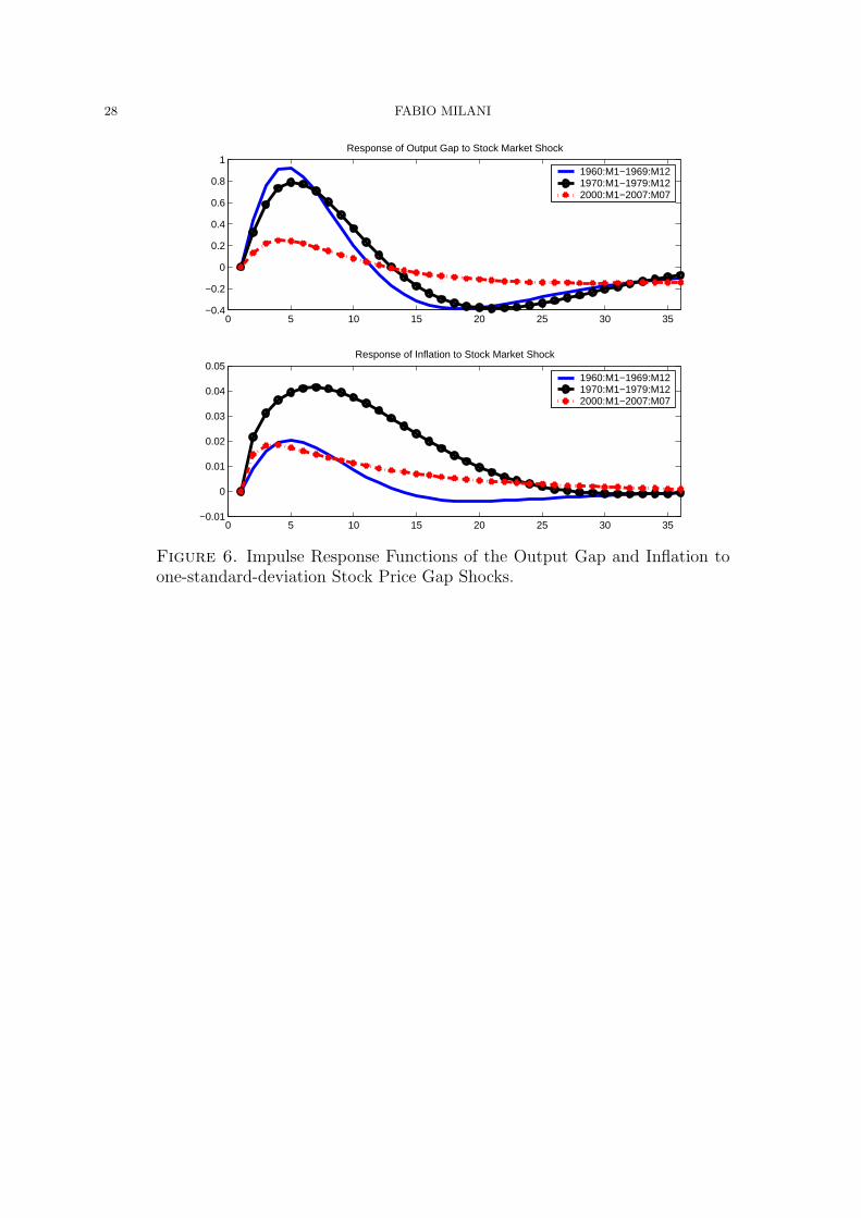
Figure 5 exhibits the impulse response of the output gap to a stock price shock as it varies

over the sample. In the early part of the sample and until the early 1980s, stock market

shocks induce a sharp increase in output that lasts about a year, before falling below its

initial level and reverting to zero in less than three years. The effect becomes much smaller

in the second half of the sample. Inflation is also affected by stock market shocks: the

effect is larger in the 1970s (figure 6). These shocks explain, on average, around 10% of the

variance in inflation (Table 4).

Biørnland and Leitemo (2008) discuss how stock price shocks that produce a permanent

effect on output may be interpreted as “news” shock, while shocks that produce only a

transitory effect are more evocative of sunspot shocks. As them, I find only transitory effects

20The effect of stock prices through expectations, rather than through a direct wealth channel, is consistentwith the microeconometric evidence that uncovers a similar consumption response between households thatown or do not own equities to stock price changes (e.g., Otoo, 1999).

21Doan, Litterman, and Sims (2003), in a paper with unrelated focus, find similar evidence that stockprice shocks are important in a structural VAR on data up to 1983. The percentage of variance they explainamounts to 30-40% after 1960 and it was already declining from more than 60% in their 1948:M7-1960:M1sample.


on output: these results seem to confirm, in a structural model, Biørnland and Leitemo’s

finding that stock price shocks may be better understood as non-fundamental sunspots.

But why has the role of stock market shocks faded over time?

One possible interpretation is that economic agents slowly learned over the sample and

are converging to the true estimate of a wealth channel close to zero.

Maybe more likely, the decline in the stock market effects on the real economy may be

related to the “Great Moderation”. The standard deviation of the output gap measure

has fallen from 2.68 before 1984 to 1.24 afterwards, while the standard deviation of the

stock price gap did not experience a similar decline (it went from 8.61 to 6.60). The stock

market has remained volatile, but the volatility of asset price fluctuations has not translated

into macroeconomic volatility. The improved monetary policy, which is one of the major

candidates as driver of the Great Moderation, may have induced agents to expect small

deviations of output from potential and, therefore, it may have reduced the usefulness of

asset prices in forecasting the output gap.

4.3.1. Stock Market and the Propagation of Shocks. The stock market, mainly through its

effect on expectations, plays also a significant role in propagating non-financial shocks. Figure

7 displays the mean impulse responses, across sub-samples, of the output gap to a monetary

policy shock for the baseline model and for an alternative model in which the effect of stock

prices on expectations is shut down. In periods when economic agents give a relatively large

weight to stock prices in their forecasting model, the stock market considerably amplifies

the propagation of monetary policy shocks (this is evident in the 1960s and 1970s). A

monetary contraction, in fact, depresses both output and stock prices, which in turn, through

their effect on expectations, cause an even larger reduction in output. The initial effect is,

therefore, magnified. The role of the stock market, however, varies over the sample. In the

1984-1999 sub-sample, the model that allows for stock price effects on expectations displays

an attenuated and more transient response (this is mostly due to a perceived negative effect

of past output on current stock prices in this period, which weakens the original output

effect). Finally, when agents’ beliefs assign a small weight to asset prices in their perceived

law of motion (as in the 2000-2007 period), the impulse responses with or without stock

price effects are virtually indistinguishable.

14 FABIO MILANI

If the stock market channel is entirely shut down, demand shocks would pick up most of

the effect of stock price shocks in explaining output fluctuations (their importance rises to

60% in the first half and 75% in the second half). Monetary policy shocks would also matter

more and they would account for a larger part of the variation in inflation.

4.4. Does Monetary Policy React to Stock Market Fluctuations? The full-sample

estimates indicate that monetary policy has responded to the stock price gap. The posterior

mean estimate for χs in table 2 equals 0.139.

The feedback to the stock price gap is much lower (χs = 0.034) in the post-1984 sample:

this is consistent with the reduced influence of stock prices on output expectations and with

the common perception that Fed’s policy under Greenspan did not react to the bubble in the

1990s. Moreover, if the estimation is repeated using a Taylor rule that responds to forecasts

of inflation and the output gap (i.e., to Etπt+1 and Etxt+1, assuming that the Fed uses the

same forecasting model (2.10) as the private sector), rather than to their lagged values, the

response to the stock price gap is quite precisely estimated around zero (and the model fit

improves). This signals that policy reacts to stock prices only to the extent that they act as

leading indicators of future inflation and real activity, but no separate response exists.22

Recent papers find that if central banks react to asset prices, they may increase the

chances of indeterminacy in the economy. Carlstrom and Fuerst (2007) find determinacy

only if the response to asset prices remains below a certain threshold. Airaudo et al. (2007),

in the same model used in this paper, study determinacy and learnability conditions. They

similarly show that a positive reaction to the stock price gap may enlarge the indeterminacy

region. Indeterminacy is also more likely when γ is close to 0, as estimated in this paper.

The post-1984 estimates, however, indicate that Federal Reserve policy, by not actively

targeting stock prices, has likely been conducive to determinacy and E-stability.

4.5. The Effect of Monetary Policy and Macro Shocks on Stock Prices. Figure 8

presents the impulse responses of the stock price gap to one-standard-deviation monetary

policy, demand, and supply shocks. Stock prices seem more responsive to monetary policy

surprises in the 1960-1970s: a contractionary shock leads to a decline in stock prices with a

22Fuhrer and Tootell (2008) similarly find little evidence of an independent response to stock values whenGreenbook forecasts are included in Taylor rules.


negative peak seven months after the shock. The decline would be even more pronounced

if examined on 1970s data alone. The response in the latest part of the sample, instead,

is much smaller (the plotted response, however, conceals some variation that exists in the

post-1984 period).23 This may suggest a recent more limited effect of monetary policy, but

it might also reflect the difficulty in identifying monetary policy shocks in the second part

of the sample on monthly data (responses that may be found on high-frequency data may

have become extremely short-lived and may be lost in the monthly averaging).

Shocks in the natural interest rate lead to an immediate jump in the stock price gap, which

turns negative after six-eight months, before reverting to zero. Inflationary shocks lead to a

decline in the stock price gap, with a less sluggish adjustment in the post-1984 sample.

Table 4 reports the outcome of the forecast error variance decomposition at alternative

horizons. Regarding the stock price gap, in the 1960-1970s, monetary policy shocks ac-

counted for up to 7.5% of the variance, demand shocks for 6.2%. Fluctuations in the stock

market are mostly driven by shocks that originate in the stock market. In the second half

of the sample, monetary policy shocks account for up to 9.7% of fluctuations, and demand

shocks for more than 20%: the stock market hence appears not as isolated from the rest of

the economy as in the past.

5. Conclusions

The paper has provided evidence from a structural model on the empirical relevance

of interactions between macroeconomic variables and the stock market. One of the main

channels that are usually emphasized in policy discussions, the wealth channel, appears

modest. But the stock market plays a significant role through its impact on expectations

about future real activity.

Monetary policy seems to have reacted to stock price fluctuations, but, in the post-1984

sample, only to the extent that they influence output and inflation forecasts. A monetary

policy response may be justified if non-rational movements in the stock market affect expec-

tations, as found in the data, and if non-fundamental stock market shocks are an important

source of fluctuations. But both these effects are now less important. Still, the welfare

23The small response may be consistent with Davig and Gerlach (2007)’s estimate of a distinct regime inthe late 1990s-early 2002, in which stock prices’ response to policy shocks is insignificant and volatile.

16 FABIO MILANI

implications of different monetary policy rules in a model in which asset prices affect private

sector’s expectations and learning is an important topic that deserves future study.

The stock market dynamics is affected by macroeconomic fundamentals, but a large part

of fluctuations is due to non-fundamental stock price shocks. A better modeling of the stock

market, which retains second-order terms, will be needed to shed more light on the nature

of financial shocks (Challe and Giannitsarou, 2007, offer a general equilibrium framework in

this direction). Future extensions should also move away from the linear/Gaussian frame-

work: including stochastic volatility in the structural innovations, for example, would allow

researchers to study the relation between output and stock price volatility, as well as be-

tween expectations of future booms and busts and volatility. Finally, it is necessary to check

whether the evidence is robust to the use of a larger model and the inclusion of different

financial sector channels: in this respect, Christiano et al. (2008)’s findings, in a different

framework, similarly identify an important role for financial shocks.


References

[1] Adam, K., (2005). “Learning to Forecast and Cyclical Behavior of Output and Inflation”, Macroeco-nomic Dynamics, Vol. 9(1), 1-27.

[2] Adam, K., A. Marcet, and J.P. Nicolini, (2007). “Stock Market Volatility and Learning”, CEPR WorkingPaper No. 6518.

[3] Airaudo, M., S. Nistico, and L.F. Zanna (2007), “Learning, Monetary Policy, and Asset Prices”, LLEEWorking Paper No.48.

[4] An, S., and F. Schorfheide, (2007). “Bayesian Analysis of DSGE Models”, Econometric Reviews, Vol.26, Iss. 2-4, 113-172.

[5] Ando, A., and F. Modigliani, (1963). “The ‘Life Cycle’ Hypothesis of Saving: Aggregate Implicationand Tests, American Economic Review, 53(1), pp. 5584.

[6] Bernanke, B., and M. Gertler, (2001). “Should Central Banks Respond to Movements in Asset Prices?”,American Economic Review, 253-57.

[7] Bernanke, B.S., and M. Gertler, and Gilchrist, S. (1999). “The Financial Accelerator in a QuantitativeBusiness Cycle Framework,” Handbook of Macroeconomics, edition 1, volume 1, chapter 21, 1341-1393.

[8] Bernanke, Ben S. and Kenneth N. Kuttner (2003), What Explains the Stock Markets Reaction toFederal Reserve Policy?”, Journal of Finance, 60, 1221-1257.

[9] Bjørnland, H.C., and K. Leitemo, (2008). “Identifying the Interdependence between US Monetary Policyand the Stock Market”, Journal of Monetary Economics, forthcoming.

[10] Blanchard, O.J., (1981). “Output, the Stock Market, and Interest Rates,” American Economic Review,vol. 71(1), pages 132-43.

[11] Blanchard, O.J., (1985), “Debt, Deficits, and Finite Horizons”, Journal of Political Economy, 93, pp.223-247.

[12] Blanchard, O.J., and J. Galı, (2007). “The Macroeconomic Effects of Oil Price Shocks: Why are the2000s so Different from the 1970s?”, NBER Working Paper No. 13368.

[13] Branch, W., and G.W. Evans, (2007). “Asset Return Dynamics and Learning”, mimeo, UC Irvine andUniversity of Oregon.

[14] Branch, W., and G.W. Evans, (2008). “Learning about Risk and Return: A Simple Model of Bubblesand Crashes”, mimeo, UC Irvine and University of Oregon.

[15] Carlstrom, C.T., and T.S. Fuerst, (2007). “Asset Prices, Nominal Rigidities, and Monetary Policy”,Review of Economic Dynamics, vol. 10(2), 256-275.

[16] Case, K.E., J.M. Quigley, and R.J. Shiller (2005), “Comparing Wealth Effects: The Stock Market VersusThe Housing Market”, Advances in Macroeconomics, vol. 5(1).

[17] Cecchetti S G, H Genberg, J Lipsky and S Wadhwani, (2000). “Asset Prices and Central Bank Policy”,Geneva Reports on the World Economy, vol 2, Geneva: International Center for Monetary and BankingStudies, London: Centre for Economic Policy Research.

[18] Challe, E., and C. Giannitsarou, (2007). “Stock Prices and Monetary Policy Shocks: a General Equi-librium Approach”, unpublished manuscript.

[19] Chen, N.F., Roll, R., and S.A. Ross, (1986). “Economic Forces and the Stock Market,” Journal ofBusiness, vol. 59(3), pages 383-403.

[20] Christiano, L., Motto, R., and M. Rostagno, (2008). “Financial Factors in Business Cycles”, unpublishedmanuscript.

[21] Davig, T., and J.R. Gerlach, (2006). “State-Dependent Stock Market Reactions to Monetary Policy”,International Journal of Central Banking, Vol. 2(4), 65-84.

[22] Davis, M., and M.G. Palumbo (2001), “A Primer on the Economics and Time Series Econometrics ofWealth Effects”, Federal Reserve Board Finance and Economics Discussion Series No. 09.

[23] Doan, T., Litterman, R., and C.A. Sims, (1983). “Forecasting and Conditional Projection Using RealisticPrior Distributions”, Econometric Reviews, 3(1), 1-100.

[24] Duca, J.V., (2006). “Mutual Funds and the Evolving Long-Run Effects of Stock Wealth on U.S. Con-sumption”, Journal of Economics and Business, 58(3), 202-221.

18 FABIO MILANI

[25] Evans, G.W., and S. Honkapohja, (2007). “Expectations, Learning and Monetary Policy: An Overviewof Recent Research”, Bank of Finland Discussion Paper No. 32.

[26] Fischer, S., and R.C. Merton, (1984). “Macroeconomics and Finance: the Role of the Stock Market,”Carnegie-Rochester Conference Series on Public Policy, vol. 21, 57-108.

[27] Fuhrer, J., and G. Tootell, (2008). “Eyes on the prize: How did the Fed respond to the stock market?”,Journal of Monetary Economics, forthcoming.

[28] Gilchrist, S., and J.V. Leahy, (2002). “Monetary Policy and Asset Prices”, Journal of Monetary Eco-nomics, Vol. 49, Iss. 1, 75-97.

[29] Gilchrist, S., and M. Saito, (2007). “Expectations, Asset Prices and Monetary Policy: The Role ofLearning”, Asset Prices and Monetary Policy, ed. by John Campbell, Chicago: University of ChicagoPress, forthcoming.

[30] Guidolin, M., and A. Timmermann, (2007).“Properties of Equilibrium Asset Prices Under AlternativeLearning Schemes”, Journal of Economic Dynamics and Control, vol. 31, issue 1, 161-217.

[31] Hymans, S., (1970). “Consumer durable spending: Explanation and prediction”, Brookings Papers onEconomic Activity, 2, pp. 173206.

[32] Jansen, J.W. and J.N. Nahuis (2003), “The Stock Market and Consumer Confidence: European Evi-dence”, Economics Letters, 79, pp. 89-98.

[33] Lettau, M., and S. Ludvigson, (2004). “Understanding Trend and Cycle in Asset Values: Reevaluatingthe Wealth Effect on Consumption”, American Economic Review, 94(1): 276-299.

[34] Ludvigson, S., and C. Steindel, (1999). “How Important is the Stock Market Effect on Consumption?,”Economic Policy Review, Federal Reserve Bank of New York, July, pages 29-51.

[35] Milani, F., (2007). “Expectations, Learning and Macroeconomic Persistence”, Journal of MonetaryEconomics, Vol. 54, Iss. 7, Pages 2065-2082.

[36] Milani, F., (2008). “Learning, Monetary Policy Rules, and Macroeconomic Stability”, Journal EconomicDynamics and Control, forthcoming.

[37] Nistico’, Salvatore. (2005) “Monetary Policy and Stock-Price Dynamics in a DSGE Framework.” LLEEWorking Document, 28, Luiss University.

[38] Orphanides, A., and J. Williams, (2003). “Imperfect Knowledge, Inflation Expectations and MonetaryPolicy”, in Ben Bernanke and Michael Woodford, eds., Inflation Targeting. Chicago: University ofChicago Press.

[39] Otoo, M.W. (1999), “Consumer Sentiment and the Stock Market”, Federal Reserve Board Finance andEconomics Discussion Series No. 60.

[40] Poterba, J. (2000), “Stock Market Wealth and Consumption”, Journal of Economic Perspectives, 14(2),pp. 99-119.

[41] Rigobon, R., and B. Sack, (2003). “Measuring the Reaction of Monetary Policy to the Stock Market,”The Quarterly Journal of Economics, vol. 118(2), pages 639-669.

[42] Rigobon, R., and B. Sack, (2004). “The Impact of Monetary Policy on Asset Prices,” Journal of Mon-etary Economics, vol. 51(8), pages 1553-1575.

[43] Stock, J.H, and M.W. Watson, (2003). “Forecasting Output and Inflation: The Role of Asset Prices,”,Journal of Economic Literature, vol. 41(3), pages 788-829.

[44] Timmermann, A.G, (1993). “How Learning in Financial Markets Generates Excess Volatility and Pre-dictability in Stock Prices,” The Quarterly Journal of Economics, vol. 108(4), 1135-45.

[45] Woodford, M., (2003). Interest and Prices: Foundations of a Theory of Monetary Policy. Princeton:Princeton University Press.

[46] Yaari, Menahem E. (1965) “Uncertain Lifetime, Life Insurance, and the Theory of the Consumer.”Review of Economic Studies, 32.


Prior DistributionDescription Parameter Distr. Support Prior Mean 95% Prior Prob. IntervalProb. of Leaving the Mkt. γ U [0,1] 0.5 [0.025,0.975]Elast. Subst. Different. Goods θ Γ R+ 12 [3.26,26.13]Slope PC κ Γ R+ 0.25 [0.03,0.70]MP Inertia ρ B [0,1] 0.8 [0.459,0.985]MP Inflation feedback χπ Γ R+ 0.5 [0.06,1.40]MP Output Gap feedback χx Γ R+ 0.25 [0.03,0.70]MP Stock Price Gap feedback χs N R 0 [-0.29,0.29]Std. Demand Shock σr Γ−1 R+ 0.11 [0.038,0.31]Std. Stock Price Shock σe Γ−1 R+ 0.33 [0.11,0.92]Std. Supply Shock σu Γ−1 R+ 0.11 [0.038,0.31]Std. MP Shock σε Γ−1 R+ 0.11 [0.038,0.31]Autoregr. coeff. rN

t ρr B [0,1] 0.8 [0.459,0.985]Autoregr. coeff. eN

t ρe B [0,1] 0.8 [0.459,0.985]Autoregr. coeff. ut ρu B [0,1] 0.8 [0.459,0.985]Constant Gain g Γ R+ 0.031 [0.003,0.087]

Table 1 - Prior Distributions.(U= Uniform, N= Normal, Γ= Gamma, B= Beta, Γ−1= Inverse Gamma)

20 FABIO MILANI

Posterior DistributionDescription Parameter Posterior Mean 95% HPDProb. of Leaving the Mkt. γ 0.0084

(0.006)[0.0004,0.023]

Sensit. Stock Prices to Output λ 0.09(0.10)

[-0.11,0.29]

Slope PC κ 0.008(0.004)

[0.001,0.017]

MP Inertia ρ 0.986(0.004)

[0.977,0.994]

MP Inflation feedback 1 + χπ 1.39(0.20)

[1.11,1.91]

MP Output Gap feedback χx 0.19(0.09)

[0.05,0.43]

MP Stock Price Gap feedback χs 0.135(0.05)

[0.06, 0.265]

Std. Demand Shock σr 0.76(0.02)

[0.71,0.80]

Std. Stock Price Shock σe 4.15(0.13)

[3.90,4.42]

Std. Supply Shock σu 0.22(0.01)

[0.21,0.24]

Std. MP Shock σε 0.045(0.001)

[0.04,0.05]

Autoregr. coeff. rNt ρr 0.43

(0.04)[0.35,0.50]

Autoregr. coeff. et ρe 0.24(0.04)

[0.16,0.32]

Autoregr. coeff. ut ρu 0.21(0.04)

[0.13,0.28]

Constant Gain g 0.014(0.0014)

[0.011,0.017]

Wealth Effect ψ1+ψ 0.00055

(0.0007)[0.000005,0.0025]

Table 2 - Posterior Estimates.Full Sample 1960:M1-2007:M7, Baseline Case. The table shows the posterior mean (standard deviation

in brackets) and the 95% Highest Posterior Density Interval.


Post-1984 Sample Taylor rule with Expect. No Effect of st on Expect.Parameter Post. Mean 95% HPD Post. Mean 95% HPD Post. Mean 95% HPD

γ 0.0090(0.007)

[0.0004,0.026] 0.0090(0.007)

[0.0004,0.024] 0.033(0.016)

[0.002,0.062]

λ 0.095(0.20)

[-0.30,0.48] 0.09(0.20)

[-0.29,0.45] 0.055(0.11)

[-0.15,0.27]

κ 0.012(0.007)

[0.002,0.03] 0.013(0.007)

[0.002,0.03] 0.0096(0.005)

[0.0017,0.02]

ρ 0.989(0.004)

[0.98,0.995] 0.97(0.007)

[0.957,0.984] 0.987(0.005)

[0.976,0.994]

1 + χπ 1.35(0.18)

[1.1,1.79] 1.45(0.22)

[1.13,1.94] 1.377(0.20)

[1.1,1.86]

χx 0.37(0.14)

[0.17,0.72] 0.18(0.06)

[0.08,0.31] 0.19(0.1)

[0.05,0.44]

χs 0.034(0.023)

[-0.001, 0.09] −0.0001(0.007)

[-0.013,0.015] 0.132(0.05)

[0.06,0.25]

σr 0.56(0.02)

[0.52,0.61] 0.56(0.02)

[0.52,0.62] 0.70(0.02)

[0.66,0.74]

σe 4.17(0.17)

[3.85,4.53] 4.17(0.19)

[3.83,4.58] 4.12(0.13)

[3.88,4.40]

σu 0.21(0.01)

[0.19,0.23] 0.21(0.01)

[0.19,0.23] 0.23(0.007)

[0.22,0.25]

σε 0.02(0.001)

[0.018,0.022] 0.02(0.001)

[0.018,0.022] 0.046(0.001)

[0.04,0.05]

ρr 0.39(0.05)

[0.28,0.49] 0.36(0.06)

[0.26,0.47] 0.44(0.04)

[0.36,0.52]

ρe 0.24(0.05)

[0.14,0.35] 0.24(0.05)

[0.15,0.33] 0.31(0.05)

[0.21,0.41]

ρu 0.26(0.06)

[0.15,0.37] 0.25(0.05)

[0.16,0.35] 0.15(0.04)

[0.08,0.22]

g 0.0138(0.0024)

[0.009,0.019] 0.0148(0.0022)

[0.01,0.019] 0.0094(0.0017)

[0.006,0.013]ψ

1+ψ 0.00064(0.0008)

[0.000006,0.003] 0.00064(0.0008)

[0.000006,0.003] 0.0061(0.0048)

[0.00005,0.017]

Table 3 - Posterior Estimates: Alternative Models.

The table shows the posterior mean, standard deviations, and the 95% Highest Posterior Density Interval.The second and third column refer to the estimate for the 1984:M1-2007:M7 sample, the fourth and fifthcolumn to the 1984:M1-2007:M7 sample using a model with a Taylor rule that responds to expected inflationand output gap it = ρit−1 + (1− ρ)[(1 + χπ)Etπt+1 + χxEtxt+1 + χsst−1] + εt, the sixth and seventh to thefull-sample estimation of a model in which the stock price gap st is assumed not to affect economic agents’expectations in (2.10).

22 FABIO MILANI

Horizon MP Shock rNt Shock Stock Market Shock Inflation Shock

Pre-1979 Post-1984 Pre-1979 Post-1984 Pre-1979 Post-1984 Pre-1979 Post-1984Output Gap 6 0.027 0.020 0.606 0.856 0.358 0.109 0.002 0.013

24 0.156 0.133 0.425 0.726 0.408 0.129 0.004 0.012∞ 0.162 0.257 0.402 0.569 0.426 0.162 0.005 0.012

Stock Price Gap 6 0.034 0.004 0.028 0.125 0.930 0.861 0.001 0.00924 0.074 0.039 0.062 0.222 0.856 0.726 0.003 0.011∞ 0.075 0.097 0.062 0.212 0.855 0.676 0.003 0.011

Inflation 6 0.038 0.01 0.024 0.067 0.058 0.052 0.874 0.86924 0.049 0.028 0.034 0.096 0.125 0.075 0.786 0.798∞ 0.050 0.060 0.035 0.10 0.128 0.09 0.781 0.759

FFR 6 0.742 0.818 0.043 0.040 0.199 0.127 0.009 0.01424 0.429 0.651 0.072 0.107 0.483 0.227 0.009 0.014∞ 0.421 0.635 0.072 0.120 0.492 0.231 0.009 0.013

Table 4 - Forecast Error Variance Decomposition.


-8

-4

0

4

8

-40

-30

-20

-10

0

10

20

30

40

1960 1970 1980 1990 2000

Output Gap Real Stock Price Gap

Figure 1. Output Gap and Real Stock Price Gap series. Note: the series areexpressed in percentage deviations from potential; the left scale refers to the output gap,right scale to the stock price gap. The light-yellow shaded areas denote NBER recessiondates.

24 FABIO MILANI

1960 1965 1970 1975 1980 1985 1990 1995 2000 20050.01

0.02

0.03

0.04

0.05

0.06

0.07

0.08

0.09

0.1

Figure 2. Agents’ Beliefs: Perceived Sensitivity of the Output Gap to StockPrice Gap Movements. Note: The solid line denotes the posterior mean of beliefs acrossMetropolis-Hastings draws. The dotted lines denote the 2.5% and 95% error bands.


1960 1965 1970 1975 1980 1985 1990 1995 2000 2005 20100.2

0.4

0.6

0.8

1

1.2

1.4

1.6

1.8

2

2.2Baseline case with learningNo effect of stock prices on expectationsConstant effect of stock prices on expectations (as in 1965)

Figure 3. Rolling Root Mean Squared Error. Note: The graphs shows the rollingRMSE calculated using a window of 60 observations (for the first five years, the RMSE isrecursively calculated. The baseline case refers to the agents’ PLM in (2.10), the secondassuming a zero effect of the real stock price gap in the agents’ PLM, the third assuming aconstant (large) effect of the stock price gap on output expectations, which is fixed at theagents’ belief in 1965 (i.e., b12 = 0.056)

26 FABIO MILANI

Figure 4. Variance Decomposition: Variance of the output gap, xt, due tostock price gap shocks, shown across forecast horizons and over the sample.


0

12

24

36

1960

1970

1980

1990

2000

2010−0.8

−0.4

0

0.4

1

MonthsTime

IRF

Figure 5. Impulse Response Function of the Output Gap to a one-standard-deviation Stock Price Gap Shock, shown across horizons and over the sample.

28 FABIO MILANI

0 5 10 15 20 25 30 35−0.01

0

0.01

0.02

0.03

0.04

0.05Response of Inflation to Stock Market Shock

1960:M1−1969:M121970:M1−1979:M122000:M1−2007:M07

0 5 10 15 20 25 30 35−0.4

−0.2

0

0.2

0.4

0.6

0.8

1Response of Output Gap to Stock Market Shock

1960:M1−1969:M121970:M1−1979:M122000:M1−2007:M07

Figure 6. Impulse Response Functions of the Output Gap and Inflation toone-standard-deviation Stock Price Gap Shocks.


0 20 40 60 80 100 120

−0.4

−0.2

0Sample: 1960:M1−1969:M12

Model with Effect of st on Expectations

No Effect of st on Expectations

0 20 40 60 80 100 120

−0.4

−0.2

0Sample: 1970:M1−1979:M12

0 20 40 60 80 100 120

−0.4

−0.2

0

Sample: 1984:M1−1999:M12

0 20 40 60 80 100 120

−0.4

−0.2

0 Sample: 2000:M1−2007:M07

Figure 7. Impulse Response Functions of the Output Gap to a one-standard-deviation Monetary Policy Shock. Note: The solid line denotes the impulse responsesin the baseline estimated model, which includes a direct wealth effect and allows for an effectof stock prices on expectations. The dashed line refers to an alternative model, in which theeffect of stock prices on expectations is shut down.

30 FABIO MILANI

Figure 8. Impulse Response Functions of the Real Stock Price Gap to one-standard-deviation Monetary Policy, Natural Rate, Stock Market, and Cost-Push Shocks.

learning about the interdependence between the macroeconomy

Documents