Learning Attributes from Human Gaze

Nils Murrugarra-Llerena Adriana KovashkaDepartment of Computer Science

University of Pittsburgh{nineil, kovashka}@cs.pitt.edu

Abstract

While semantic visual attributes have been shown usefulfor a variety of tasks, many attributes are difficult to modelcomputationally. One of the reasons for this difficulty isthat it is not clear where in an image the attribute lives. Wepropose to tackle this problem by involving humans moredirectly in the process of learning an attribute model. Weask humans to examine a set of images to determine if agiven attribute is present in them, and we record wherethey looked. We create gaze maps for each attribute, anduse these gaze maps to improve attribute prediction mod-els. For test images we do not have gaze maps available,so we predict them based on models learned from collectedgaze maps for each attribute of interest. Compared to sixbaselines, we improve prediction accuracies on attributesof faces and shoes, and we show how our method mightbe adapted for scene images. We demonstrate additionaluses of our gaze maps for visualization of attribute modelsand learning “schools of thought” between users in termsof their understanding of the attribute.

1. IntroductionSemantic visual attributes (such as “metallic” or “smil-

ing”) have been used for a variety of tasks: as a low-dimensional representation for object recognition [7, 26, 33,53, 16], as a textual representation used to recognize previ-ously unseen categories [7, 26, 31, 16, 27], as a supervisionmodality for active learning [24, 32], etc.

However, unlike object categories, attributes are notwell-defined. To see why, consider the following thoughtexperiment. If a person is asked to draw a “boot”, the draw-ings of different people will likely not differ very much. Butif a person is asked to draw what the attributes “formal” or“feminine” mean, drawings will vary. Drawings of a “for-est” will likely all include a number of trees, but drawingsof a “natural”, “open-area”, or “cluttered” scene will differgreatly among artists. Finally, if humans are asked to drawor even pick from a set of male actors an “attractive” or

Q: Is it pointy?A: No.

Q: Is she attractive?A: Yes.

Q: Is she chubby?A: Yes.

Q: Is it formal?A: Yes.

Figure 1: We learn the spatial support of attributes by askinghumans to judge if an attribute is present in training images.We use this support to improve attribute prediction.

“masculine” person, responses will differ more than if theywere asked to draw or select a “man”.

Since attributes are less well-defined, capturing themwith computational models poses a different set of chal-lenges than capturing object categories does. There is adisconnect between how humans and machines perceive at-tributes, and it negatively impacts tasks that involve com-munication between a human and a machine, since the ma-chine may not understand what a human user has in mindwhen referring to a particular attribute. Since attributes arehuman-defined, the best way to deal with their ambiguity isby learning from humans what these attributes really mean.

We propose to learn attribute models using human gazemaps that show which part of an image contains the at-tribute. To obtain gaze maps for each attribute, we con-duct human subject experiments where we ask viewers toexamine images of faces, shoes, and scenes, and determineif a given attribute is present in the image or not. We usean inexpensive GazePoint eyetracking device which is sim-ply placed in front of a monitor to track viewers’ gaze, andrecord the locations in the image that had some number offixations. We aggregate the gaze collected from multiplepeople on training images, to obtain an averaged gaze mapper attribute that we use to extract features from both train-ing and test images. We also experiment with learning asaliency model that predicts which pixels will be fixated. Tocapture the potential ambiguity and visual variation withineach attribute, we cluster the positive images per attributeand their corresponding gaze locations, and obtain multiplegaze maps per attribute. We create one classifier per gaze

map which only uses features from the region under non-zero gaze map values, for both training and testing.

The gaze maps that we learn from humans indicate thespatial support for an attribute in an image and allow usto better understand what the attribute means. We use gazemaps to identify regions that should be used to train attributemodels. We show this achieves competitive attribute predic-tion accuracy compared to six methods, five of which arealternative ways to select relevant features. We also demon-strate additional applications showing how our method canbe used to visualize attribute models, and how it can be em-ployed to discover groups among users in terms of their un-derstanding of attribute presence.

The main contribution of our work is a new method forlearning attribute models, using inexpensive but rich data inthe form of gaze. We show that our method successfullydiscovers the spatial support of attributes. Despite the closeconnection between attributes and human communication,gaze has never been used to learn attribute models before.

2. Related WorkAttributes. Semantic visual attributes are properties ofthe visual world, akin to adjectives [26, 7, 1, 33]. In thiswork, we focus on modeling attributes as binary categories[26, 7, 1, 33]. Attributes bring recognition closer to human-like intelligence, since they allow generalization in the formof zero-shot learning, i.e. learning to recognize previouslyunseen categories using a textual attribute-based descrip-tion and prediction models for these attributes learned onother categories [26, 7, 31, 16]. Attributes have also beenshown useful for actively learning object categories [32],scene recognition [33], and action recognition [27].Attribute naming and ambiguity. [30, 33] propose howto develop an attribute vocabulary. [20, 21] show attributescan be subjective and there exist “schools of thought” interms of how users use an attribute word. In other words,users can be grouped in terms of how they respond to ques-tions about the presence or absence of attributes, and howthey use the attribute name. Some work discovers non-semantic nameless attributes [53, 35, 38], but for tasks in-volving search and zero-shot learning we require attributesthat have human-given names.Learning and localizing attribute models. Some workstudies specifically how to learn accurate attribute models.For example, [2, 47, 8, 39, 12, 52] model attributes jointly.[16] improve attribute predictions by decorrelating the useof features by different attribute models, and [9] improveattribute prediction accuracy by finding a feature represen-tation that is invariant across categories. In the domain ofrelative attributes [31], which we do not study, [37] discoverparts that improve relative attribute prediction accuracy. It isunclear whether the discovered parts capture the true mean-ing of attributes as humans perceive them, or simply exploit

image features which are correlated [16] with the attributeof interest, but are not part of the human perception of theattribute.1 Further, [37]’s method is not applicable to bi-nary attributes and requires pre-trained facial landmark de-tectors. In recent work, [48] propose to discover the spatialextent of relative attributes, and apply their method to im-ages of shoes and faces as we do. They find spatial extent bybuilding “visual chains” that capture the commonalities be-tween images which flow from ones having the attribute toa strong degree, to those that have it less. While we modelattributes as binary properties (in contrast to [48]), and usehuman insight to learn where an attribute lives, [48] is themost related work to ours so we compare to it in Sec. 4.

Other recent work applies deep neural networks to pre-dict attributes [39, 40, 6, 46, 8]. While deep nets can im-prove the discriminativity of attribute models, they do notexploit human supervision on the meaning or spatial sup-port of attributes. Thus, progress in deep nets is orthogonalto the objective of our study. We show that even when deepfeatures are employed, using gaze maps to determine thespatial support of attributes improves performance.Using humans to select relevant regions. [44] pair twohumans in an image-based guessing game, where the goalis for the first person to reveal such image regions that al-low the second person to most quickly guess the categoryof the image. The revealed regions are then assumed to bethe most relevant for the category of interest. [3, 4] proposea single-player guessing game called “Bubbles,” where theplayer must reveal as few circular regions of an image aspossible, in order to match that image to one of two cate-gories with several examples shown. There are three im-portant differences between our work and [44, 3, 4]: (1)These approaches are used to learn objects, not attributes,and attributes have much more ambiguous spatial support;(2) They require that a human should click on a relevant im-age region, which means that the user is consciously awareof what the relevant regions are, whereas in our approacha human uses her potentially subconscious intuition aboutwhat makes an image “natural”, “formal”, or “chubby”; and(3) Clicking or drawing requires a bit more effort (lookingis easier than moving one’s hand to use the mouse).

Our method can be seen as a form of annotator ratio-nales [55, 5], which are annotations that humans provide toteach the classifier why a category is present. For example,the user can mark which regions of the face make a person“attractive”. However, providing gaze maps by looking ismuch faster than drawing rationales (see Sec. 3.2).Gaze and saliency. [29] use human gaze to reduce theeffort required in obtaining data for object detectors. Theybuild bounding boxes from locations in a photo where a userfixates when judging which of two categories is portrayed

1This is also true for attention networks [42, 15] as they are data-driven,not based on human intuition.

in the image. [54] argue that using gaze can improve objectdetection—bounding box predictions that do not align withfixations can be pruned. They also use a gaze-based featureto classify detections into true and false positives, but onlyshow small gains in detection accuracy.

In addition to gaze, saliency examines where a viewerwill fixate in an image [14, 34, 28, 11, 19, 10, 18, 13]. Weuse [19]’s method to predict gaze maps for novel images.No prior work uses gaze to learn attribute models.

3. Approach

We first describe our datasets (Sec. 3.1) and how we col-lect gaze data from human subjects (Sec. 3.2). In Sec. 3.3,we discuss how we compute one or multiple gaze templatesper attribute, and in Sec. 3.4, we describe how we use thetemplates to restrict the range of an image from which an at-tribute model is learned. Finally, in Sec. 3.5, we show howwe predict an individual gaze template for each test image.

Like [48], our method is designed for images whichcontain a single object, specifically faces and shoes. SeeSec. 4.2 for a preliminary adaptation of our work for scenes.

3.1. Datasets

We use two attribute datasets: the Faces dataset of [25](also known as PubFig), and the Shoes dataset of [22].All images are of the same square size (200x200 pixelsfor faces and 280x280 for shoes). The attributes we useare: for Shoes, “feminine”, “formal”, “open”, “pointy”,and “sporty”; and for Faces, “Asian”, “attractive”, “baby-faced”, “big-nosed”, “chubby”, “Indian”, “masculine”, and“youthful”. Like [48], we consider a subset of all attributes,in order to focus the analysis towards attributes whose spa-tial support does not seem obvious, i.e. it could not be pre-dicted from the attribute name alone. This allows insightinto the meaning of some particularly ambiguous attributes(e.g. “formal”, “feminine” and “attractive”). We also se-lected some attributes (“pointy” and “big-nosed”) wherewe had a fairly confident estimate of where gaze locationswould be. This allows us to qualitatively evaluate the col-lected gaze maps via their alignment with the expected gazelocations. The annotation cost per attribute is small, about1 minute per image-attribute pair (see below).

We select 60 images total per attribute. In order to getrepresentative examples of each attribute, we sample: (a)30 instances where the attribute is definitely present, (b) 18instances where it is definitely not present, and (c) 12 in-stances where it may or may not be present. For Faces, weuse the provided SVM decision values to select images inthese three categories. For Shoes, we use the ordering often shoe categories from most to least having each attribute,which we map to individual images using their class labels.

3.2. Gaze data collection

We employ a $495 GazePoint GP3 eye-tracker device2 tocollect gaze data from 14 participants. The 320x45x40mmeye-tracker is placed in front of a monitor, and the partic-ipants do not have to wear it, in contrast to older devices.Gaze data can also be collected via a webcam; see [50].

Our experiment begins with a screening phase in whichwe show ten images to each participant and ask him/her tolook at a fixed region in the image that is marked by a redsquare, or to look at e.g. the nose or right eye for faces. Ifthe fixated pixel locations lie within the marked region, theparticipant moves on to the data collection session. The lat-ter consists of 200 images organized in four sub-sessions. Inorder to increase the participants’ performance, we allow afive-minute break between sub-sessions. We ask the viewerwhether a particular attribute is present in a particular im-age which we then show him/her. The participant has twoseconds to look at the image and answer. His/her gaze lo-cations and answers are recorded. We obtain 2.5 gaze mapson average, for each image-attribute question.

Of the 200 images, 20 are used for validation. If thegaze fixations on some validation image are not where theyshould be, we discard data from the annotator that followsthat validation image and precedes the next one.

Each experiment took one hour, for a total of 14 hoursof human time. Thus, obtaining the gaze maps for each ofour 13 attributes took a short amount of time, about onehour per attribute or one minute per image-attribute pair.Our collected gaze data is available on our website3. Notethat viewing an image is faster than drawing a rationale (45seconds), so we save time and money compared to [5].

In contrast to our approach, some saliency work [18, 13]approximates gaze with mouse clicks, but as argued in re-lation to region selection methods (Sec. 2), clicks requireconscious awareness of what makes an image “formal” or“baby-faced”, which need not be true for attributes.

3.3. Generating gaze map templates

The gaze data and labels are collected jointly but aggre-gated separately for each attribute. The format of a recordedgaze map is an array of coordinates (x, y) of the image beingviewed. We convert this to a map with the same size as theimage, with a value of 1 or 0 per pixel denoting whether thepixel was fixated or not. First, the gaze maps across all im-ages that correspond to positive attribute labels are OR-ed(the maximum value is taken per pixel) and divided by themaximum value in the map. Thus we arrive at a gaze mapgmm for the attribute m with values in the range [0, 1]. Sec-ond, a binary template btm is created using a threshold oft = 0.1 on gmm. All locations greater than t are marked as

2http://www.gazept.com/product/gazepoint-gp3-eye-tracker/3http://www.cs.pitt.edu/∼nineil/gaze proj/

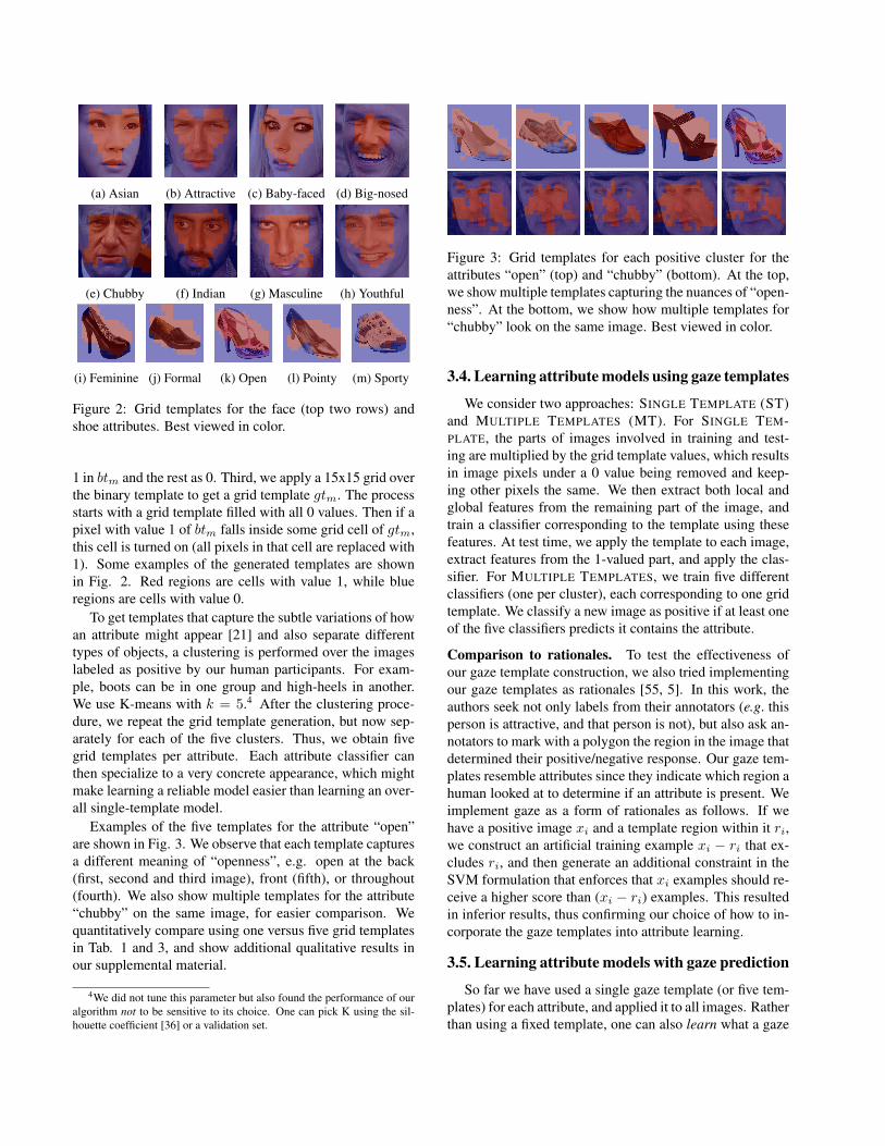
(a) Asian (b) Attractive (c) Baby-faced (d) Big-nosed

(e) Chubby (f) Indian (g) Masculine (h) Youthful

(i) Feminine (j) Formal (k) Open (l) Pointy (m) Sporty

Figure 2: Grid templates for the face (top two rows) andshoe attributes. Best viewed in color.

1 in btm and the rest as 0. Third, we apply a 15x15 grid overthe binary template to get a grid template gtm. The processstarts with a grid template filled with all 0 values. Then if apixel with value 1 of btm falls inside some grid cell of gtm,this cell is turned on (all pixels in that cell are replaced with1). Some examples of the generated templates are shownin Fig. 2. Red regions are cells with value 1, while blueregions are cells with value 0.

To get templates that capture the subtle variations of howan attribute might appear [21] and also separate differenttypes of objects, a clustering is performed over the imageslabeled as positive by our human participants. For exam-ple, boots can be in one group and high-heels in another.We use K-means with k = 5.4 After the clustering proce-dure, we repeat the grid template generation, but now sep-arately for each of the five clusters. Thus, we obtain fivegrid templates per attribute. Each attribute classifier canthen specialize to a very concrete appearance, which mightmake learning a reliable model easier than learning an over-all single-template model.

Examples of the five templates for the attribute “open”are shown in Fig. 3. We observe that each template capturesa different meaning of “openness”, e.g. open at the back(first, second and third image), front (fifth), or throughout(fourth). We also show multiple templates for the attribute“chubby” on the same image, for easier comparison. Wequantitatively compare using one versus five grid templatesin Tab. 1 and 3, and show additional qualitative results inour supplemental material.

4We did not tune this parameter but also found the performance of ouralgorithm not to be sensitive to its choice. One can pick K using the sil-houette coefficient [36] or a validation set.

Figure 3: Grid templates for each positive cluster for theattributes “open” (top) and “chubby” (bottom). At the top,we show multiple templates capturing the nuances of “open-ness”. At the bottom, we show how multiple templates for“chubby” look on the same image. Best viewed in color.

3.4. Learning attribute models using gaze templates

We consider two approaches: SINGLE TEMPLATE (ST)and MULTIPLE TEMPLATES (MT). For SINGLE TEM-PLATE, the parts of images involved in training and test-ing are multiplied by the grid template values, which resultsin image pixels under a 0 value being removed and keep-ing other pixels the same. We then extract both local andglobal features from the remaining part of the image, andtrain a classifier corresponding to the template using thesefeatures. At test time, we apply the template to each image,extract features from the 1-valued part, and apply the clas-sifier. For MULTIPLE TEMPLATES, we train five differentclassifiers (one per cluster), each corresponding to one gridtemplate. We classify a new image as positive if at least oneof the five classifiers predicts it contains the attribute.

Comparison to rationales. To test the effectiveness ofour gaze template construction, we also tried implementingour gaze templates as rationales [55, 5]. In this work, theauthors seek not only labels from their annotators (e.g. thisperson is attractive, and that person is not), but also ask an-notators to mark with a polygon the region in the image thatdetermined their positive/negative response. Our gaze tem-plates resemble attributes since they indicate which region ahuman looked at to determine if an attribute is present. Weimplement gaze as a form of rationales as follows. If wehave a positive image xi and a template region within it ri,we construct an artificial training example xi − ri that ex-cludes ri, and then generate an additional constraint in theSVM formulation that enforces that xi examples should re-ceive a higher score than (xi − ri) examples. This resultedin inferior results, thus confirming our choice of how to in-corporate the gaze templates into attribute learning.

3.5. Learning attribute models with gaze prediction

So far we have used a single gaze template (or five tem-plates) for each attribute, and applied it to all images. Ratherthan using a fixed template, one can also learn what a gaze

map would look like for a novel test image. We constructa model following Judd’s simple method [19], by inputting(1) our training gaze templates, from which 0/1 gaze labelsare extracted per pixel, and (2) per-pixel image features (thesame feature set as in [19] including color, intensity, orien-tation, etc; but excluding person and car detections). Thissaliency model learns an SVM which predicts whether eachpixel will be fixated or not, using the per-pixel features. Welearn a separate saliency model for each attribute.

Data: Training grid templates templatestrain,m forattribute m; test image i

Result: Template for the test image templatei, to beused for feature extraction

1 Train a saliency model using templatestrain,m;2 Apply saliency model to i to predict gaze map gmi

m;3 for u ∈ {0.1, 0.2, . . . , 0.9} do4 r ← Threshold gmi

m at u;5 scoreu ← similarity of r and templatestrain,m6 end7 fu← Set the final threshold to argmaxu(scoreu);8 templatei ← Apply threshold fu to gaze map gmi

m

Algorithm 1: Predicting a gaze template using saliency.

For each attribute, as outlined in Alg. 1, we first learna saliency model. Then we predict a real-valued saliencyscore for each pixel in each test image. Finally, we convertthis real-valued saliency map to a binary template. To gen-erate the latter, we consider thresholds u between 0.1 and0.9. To score each u, we apply it to the predicted gaze tem-plate for our test image to obtain a binary test template. Wecompute the similarity between that test template and thetraining binary templates (Sec. 3.3), as the intersection overunion of the 1-valued regions. Finally, we fix our choice ofthe threshold u to the one with the highest similarity score.

Once we have the binary grid template for the test image,we can extract features from it as in Sec. 3.4, only from thearea predicted to have fixations on it. However, the size ofthe gaze template on test images is no longer guaranteedto be the same as the size of the template on training im-ages, so we have a feature dimensionality mismatch. Thus,we opt for a bag-of-visual-words representation over denseSIFT features (from the part of the image under positivetemplate values in the train/test images) and a vocabularyof 1000 visual words. Then, we build a new classifier us-ing the templates on the training data as discussed above,and apply this model to the features extracted from ournew predicted grid template. We call this approach SINGLETEMPLATE PREDICTED (STP) or MULTIPLE TEMPLATESPREDICTED (MTP), depending on whether a single or mul-tiple templates were used per attribute at training time. Thenames denote that at test time, we use a predicted template.

4. ResultsIn this section, we present a comparison (Sec. 4.1) of

our approach against six different baselines on the task ofattribute prediction, five of which are alternative methodsto select relevant regions in the image from which to extractfeatures. We also include two additional applications: usinggaze templates to visualize attribute models (Sec. 4.3), anddiscovering “schools of thought” among annotators whichdenote how they perceive attribute presence (Sec. 4.4). Weprimarily test our approach on the Faces and Shoes datasets,but in Sec. 4.2, we show an adaptation of our approach forscene attributes.

4.1. Attribute prediction

We build attribute prediction models using both stan-dard vision features and features extracted from convolu-tional neural networks (CNNs). We use HOG+GIST con-catenated, the fc6 layer of CaffeNet [17], and dense SIFTbag-of-words extracted in stride of 10 pixels at a single scaleof 8 pixels. Following [41], we use CaffeNet’s fc6 since fc7and fc8 may be capturing full objects and not be very usefulfor learning attributes.

Our training data consists of the images chosen for thegaze data collection experiments (Sec. 3.1), for a total of300 for shoes and 480 for faces. The training labels arethose provided by our human subject annotators. We per-form a majority vote over the labels in case the annotatorswho labeled an image disagree over its label. We might havemore positive images for an attribute than we have nega-tives, so we set the SVM classifier penalty on the negativeclass to the ratio of positive images to negative images. Weuse a linear SVM, and employ a validation set to determinethe best value of the SVM cost C in the range [0.1, 1, 10,100], separately for each attribute.

The test data consists of 341 images from Shoes and 660from Faces. The test labels are those that came with thedataset. We pool together positive and negative test data fordifferent attributes, so we often have significantly more neg-atives than positives for any given attribute. Thus, we usethe F-measure because it more precisely captures accuracywhen the data distribution is imbalanced.

Our proposed techniques for computing the spatial sup-port of an attribute and extracting features accordingly,MULTIPLE TEMPLATES and MULTIPLE TEMPLATES PRE-DICTED, as well as their simplified versions SINGLE TEM-PLATE and SINGLE TEMPLATE PREDICTED, were com-pared with the following baselines:

• using the whole image for both training and testing(WHOLE IMAGE);

• DATA-DRIVEN, a baseline which selects features us-ing an L1-regularizer over features extracted on a

grid, then sets grid template cells on/off depending onwhether at least one feature in that grid cell received anon-zero weight from the regularizer (note we do thisonly for localizable features);

• UNSUPERVISED SALIENCY, a baseline which predictsstandard saliency using a state-of-the-art method [18]5

but without training on our attribute-specific gaze data,and the resulting saliency map is then used to computea template mask;

• RANDOM, a baseline which generates a random tem-plate over a 15x15 grid, where the number of 1-valuedcells is equal to the number of 1-valued cells in thecorresponding SINGLE TEMPLATE template; and

• an ensemble of random template classifiers (RANDOMENSEMBLE), which is the random counterpart to theensemble used by MULTIPLE TEMPLATES.

Finally, we compare our method to the SPATIAL EX-TENT (SE) method of Xiao and Lee [48] which discoversthe spatial extent of relative attributes. While we do notstudy relative attributes, this is the work that is most rele-vant to our approach, thus prompting the comparison. [48]form “visual chains” from which they then build heatmapsshowing which regions in an image are most responsible forattribute strength. We are only able to perform a comparisonfor attributes that have relative annotations on our datasets,which we take from [23, 31]. We use these heatmaps assaliency predictions, which in turn are used to mask theimage and perform feature selection and attribute predic-tion (with the SVM cost C chosen on a validation set). Weuse dense SIFT and bag-of-words as for our SINGLE TEM-PLATE PREDICTED.

In Tables 1 and 2, we show results for SINGLE TEM-PLATE and MULTIPLE TEMPLATES, for HOG+GIST andfc6, respectively. In all tables, “total avg” is the mean overthe two per-attribute “avg” values above (for shoe and faceattributes, respectively). Our MT performs better than theother approaches. In Tab. 1, MT improves the performanceon shoes by 6 points or 10% (=0.66/0.60-1) relative to thesecond-best method, and on faces, it improves performanceby 3 points or 7%. In Tab. 2, our method improves perfor-mance by 2% on shoes and 7% on faces. Our MT ap-proach captures the different meanings that an attribute canhave and its possible locations. In contrast, ST imposes afixed template and ignores possible shades of meaning anddistinctions between the images viewed.

In Tab. 3, we examine the performance of SINGLETEMPLATE PREDICTED and MULTIPLE TEMPLATES PRE-DICTED. We observe that predicting the gaze map, as op-

5We used the authors’ online demo to compute saliency on our images,as code was not available.

WI ST MT DD US R RE(ours)

feminine 0.80 0.78 0.71 0.74 0.79 0.74 0.75formal 0.78 0.81 0.80 0.79 0.77 0.77 0.77open 0.52 0.53 0.57 0.45 0.55 0.51 0.51

pointy 0.17 0.17 0.46 0.00 0.10 0.14 0.10sporty 0.74 0.70 0.76 0.72 0.71 0.72 0.72

avg 0.60 0.60 0.66 0.54 0.58 0.58 0.57Asian 0.24 0.33 0.30 0.22 0.25 0.21 0.21

attractive 0.71 0.74 0.81 0.71 0.73 0.75 0.75baby-faced 0.03 0.06 0.04 0.06 0.06 0.06 0.06big-nosed 0.47 0.35 0.52 0.41 0.39 0.40 0.31

chubby 0.46 0.46 0.43 0.38 0.39 0.43 0.44Indian 0.24 0.21 0.22 0.18 0.24 0.25 0.27

masculine 0.69 0.71 0.77 0.69 0.71 0.73 0.75youthful 0.69 0.65 0.7 0.68 0.67 0.68 0.68

avg 0.44 0.44 0.47 0.42 0.43 0.44 0.43total avg 0.52 0.52 0.57 0.48 0.51 0.51 0.50

Table 1: F-measure using HOG+GIST features. WI =WHOLE IMAGE, ST = SINGLE TEMPLATE, MT = MUL-TIPLE TEMPLATES, DD = DATA-DRIVEN, US = UNSU-PERVISED SALIENCY, R = RANDOM, RE = RANDOM EN-SEMBLE. Bold indicates best performer excluding ties.

WI ST MT US R RE(ours)

feminine 0.77 0.73 0.66 0.70 0.69 0.74formal 0.63 0.57 0.61 0.58 0.59 0.58open 0.51 0.51 0.51 0.49 0.47 0.53

pointy 0.19 0.18 0.38 0.17 0.18 0.13sporty 0.82 0.78 0.79 0.77 0.67 0.69

avg 0.58 0.55 0.59 0.54 0.52 0.53Asian 0.25 0.30 0.22 0.26 0.21 0.24

attractive 0.72 0.73 0.81 0.77 0.71 0.73baby-faced 0.08 0.12 0.09 0.10 0.09 0.09big-nosed 0.46 0.44 0.67 0.44 0.40 0.31

chubby 0.42 0.37 0.41 0.35 0.34 0.32Indian 0.28 0.13 0.27 0.22 0.16 0.13

masculine 0.7 0.67 0.71 0.66 0.69 0.73youthful 0.65 0.60 0.68 0.58 0.61 0.64

avg 0.45 0.42 0.48 0.42 0.40 0.40total avg 0.51 0.49 0.54 0.48 0.46 0.47

Table 2: F-measure using fc6. See legend in Tab. 1.

posed to using a fixed map, only helps to improve the per-formance of the proposed feature selection approach on afew attributes (“formal”, “Asian” and “masculine” for STPvs ST, and “feminine” and “baby-faced” for MTP vs MT).This may be because for our face and shoe data, the ob-ject of interest is fairly well-centered (although faces can berotated to some degree). We show some unthresholded pre-dicted gaze maps in Fig. 4. Note how our raw gaze mapscorrectly detect cheeks as salient for “chubbiness”, and shoe

WI ST MT STP MTP DD US SE R RE(ours) (ours)

feminine 0.83 0.80 0.60 0.78 0.62 0.68 0.63 0.79 0.78 0.82formal 0.75 0.75 0.81 0.76 0.76 0.55 0.66 0.78 0.75 0.74open 0.53 0.58 0.57 0.53 0.56 0.30 0.43 0.59 0.50 0.57

pointy 0.16 0.30 0.53 0.10 0.48 0.55 0.00 0.56 0.23 0.20sporty 0.74 0.81 0.82 0.80 0.77 0.54 0.66 0.72 0.70 0.72

avg 0.60 0.65 0.67 0.59 0.64 0.52 0.48 0.69 0.59 0.61Asian 0.22 0.28 0.32 0.30 0.26 0.24 0.29 N/A 0.23 0.24

attractive 0.61 0.80 0.84 0.80 0.82 0.69 0.84 N/A 0.76 0.77baby-faced 0.06 0.11 0.07 0.06 0.10 0.09 0.06 N/A 0.08 0.22big-nosed 0.64 0.33 0.43 0.27 0.40 0.41 0.32 N/A 0.27 0.15

chubby 0.36 0.34 0.40 0.30 0.36 0.24 0.24 0.32 0.27 0.29Indian 0.25 0.15 0.24 0.12 0.18 0.12 0.20 N/A 0.16 0.08

masculine 0.68 0.68 0.78 0.71 0.70 0.63 0.80 0.71 0.69 0.72youthful 0.65 0.62 0.66 0.58 0.63 0.53 0.60 0.69 0.61 0.60

avg 0.43 0.41 0.47 0.39 0.43 0.37 0.42 N/A 0.38 0.38total avg 0.52 0.53 0.57 0.49 0.53 0.45 0.45 N/A 0.49 0.50

Table 3: F-measure using gaze maps predicted using thesaliency method of [19]. STP = SINGLE TEMPLATE PRE-DICTED, MTP = MULTIPLE TEMPLATES PREDICTED, SE= SPATIAL EXTENT. Other abbreviations are as before.

Figure 4: Representative predicted templates for “chubby”and “pointy”. Red = most, blue = least salient.

toes and heels as salient for “pointiness”.As before, our best results are achieved by using multiple

templates. The MT method outperforms the standard wayof learning attributes, namely WI, by 10% on average.

In terms of region selection baselines, the RANDOM andRANDOM ENSEMBLE baselines perform somewhat worsethan WHOLE IMAGE. The SINGLE TEMPLATE method per-forms similar to WHOLE IMAGE (slightly better or worse,depending on the feature type). In contrast, our MULTI-PLE TEMPLATES perform much better. This indicates thatcapturing the meaning of an attribute does indeed lie in de-termining where the attribute lives, by also accounting fordifferent participants’ interpretations. The DATA-DRIVENbaseline performs weaker than the random baselines andour method, indicating the need for rich human supervision.The UNSUPERVISED SALIENCY baseline outperforms ourmethod in a few cases (e.g. “feminine”), but overall per-forms similarly to RANDOM ENSEMBLE and weaker thanour multiple template methods. Thus, attribute informationis required to learn accurate gaze templates.

The results of [48] (SPATIAL EXTENT) are better thanMT for four of the eight attributes available to test for SE,

Figure 5: Time comparison of our MT and MTP with SE.On the y-axis is the average F-measure over the attributestested. Run1, run2, and run3 use different parameter config-urations for SE (each one requiring more processing time).Our MT is more accurate than the cheaper SE versions andas accurate as the most expensive one.

but the average over the eight attributes is almost the same(ours is slightly higher). However, for each attribute, SErequired 38 hours to run on average, on 2.6GHz Xeon pro-cessor with 256GB RAM. In contrast, our method only re-quires the time to capture the gaze maps, i.e. about onehour. In Fig. 6 (a), we compare MT with different con-figurations of SE that take a different amount of time tocompute. (The results in Tab. 3 used the original most ex-pensive setting.) Overall our method has similar or betterperformance than the different runs of SE, but it requiresmuch less time.

4.2. Adaptation for scene attributes

Similar to [48], the method most relevant to our work, wehave so far only attempted our method on faces and shoes.Given our encouraging performance, we also tested it onten scene attributes [33] (see Tab. 4 for the list), using 60images per attribute for training and 700 for testing.

A direct application of our MT and MTP performedweaker or similar to WI, likely because scene images con-tain more than one object. Thus, we adapted our methodfor this dataset, using five seconds of gaze data. The in-tuition for our adapted method is as follows: For the at-tributes “natural” and “sailing”, people might look at e.g.trees and water, respectively. Thus, we can use objects ascues for where people will look. Such an approach com-putes location-invariant masks that depend on what is por-trayed, not where it is portrayed.

Our approach consist of three steps: learning an objectdetector, modeling attributes via objects, and predicting at-tributes on test images. We fine-tuned the VGG16 network[43] with object annotations from SUN [49] on images notcontained in our gaze experiments or test set. We trainedthree CNNs grouping the objects with similar bounding boxsize. To learn attributes, we first ran the object detector onour training images. For a given attribute, we counted howmany objects intersect with its gaze fixations. Next, we nor-malized these values and compiled a list of the five mostfrequently fixated, hence most relevant categories for each

Attribute Relevant objectsclimbing mountain, sky, tree, trees, buildingopen area sky, trees, grass, road, tree

cold tree, building, mountain, sky, treessoothing trees, sky, wall, floor, tree

competing wall, floor, grass, trees, treesunny sky, tree, building, grass, treesdriving sky, road, tree, trees, building

swimming tree, trees, water, sky, buildingnatural trees, tree, grass, sky, mountain

vegetation tree, trees, sky, grass, road

Table 4: The objects most often fixated per scene attribute.

(a) (b)

Figure 6: Model visualizations for (a) the attribute “baby-faced”, using whole image features (left) and our templatemasks (right), and (b) the attribute “big-nosed”.

attribute. At test time, if at least one of these is present, wepredict the attribute is present as well.

This simple approach achieves an average F-measureof 0.37, compared to 0.33, 0.34 and 0.45 for WI withHOG+GIST, dense SIFT, and fc6, respectively. It outper-forms fc6 on the attributes “driving” and “open area”. Amore elaborate approach which extracts fc6 features on agrid and masks out cells of the grid based on overlap withrelevant objects, achieves 0.40.

The objects selected per attribute are shown in Tab. 4.We observe that for “natural”, the fixated objects are trees,grass, sky and mountains; for “driving”, one of the objects isroad, for “swimming” water, and for “climbing” mountainsand buildings. This result confirms our intuition that sceneattributes can be recognized by detecting relevant objectsassociated with the attributes through gaze. In our futurework, we will formulate this intuition such that it allows usto outperform whole-image fc6 features on more attributes.

4.3. Visualizing attribute models

We conclude with two applications of our method. First,our gaze templates can be employed to visualize attributeclassifiers. We use Vondrick et al.’s Hoggles [45], a methodused for object model visualization, and apply it to attributevisualization, on (1) models learned from the whole im-age, and (2) models learned from the regions chosen byour templates. We show examples in Fig. 6. Using thetemplates produces more meaningful visualizations than us-ing the whole image. For example, for the attribute “baby-faced”, our visualization shows a smooth face-like imagethat highlights the form of the nose and the cheeks, and for“big-nosed”, we see a focus on the nose.

4.4. Using gaze to find schools of thought

Kovashka and Grauman [21] show there exist “schoolsof thought” (groupings) of users in terms of their judgmentsabout attribute presence. They discover these groupings anduse them to build accurate attribute sub-models, each ofwhich captures an attribute variation (e.g. open at the toeas opposed to at the heel). The goal is to disambiguate at-tributes and create clean attribute models. First, they builda “generic” model (by pooling labels from many annota-tors). They discover schools using the users’ labels, by clus-tering in a latent space representation for each user, com-puted using matrix factorization on the annotators’ sparselabels. Then they use domain adaptation techniques to adaptthis “generic” model towards sparse labeled data from eachschool. At test time, they apply the user’s group’s model topredict the labels on a sample from that user. We follow thesame approach, but employ gaze to discover the schools.

We factorize an (annotator, image) table where the en-try for annotator i and image j is the cluster membershipof image j, computed by clustering images using their gazemaps on positive and negative annotations separately. Thus,for each user, we capture what type of gaze maps they pro-vide, using the intuition that how a user perceives an at-tribute affects where he/she looks. On our data, the originalmethod of [21] achieves 0.37, and our gaze-based discov-ery achieves 0.40. Our method is particularly useful for theattributes “big-nosed” (0.41 vs 0.29 for [21]), “masculine”(0.40 vs 0.35), “feminine” (0.43 vs 0.36), “open” (0.58 vs0.52), and “pointy” (0.43 vs 0.36), most of which are fairlysubjective.6 This indicates using gaze is very informativefor disambiguating attributes, the original goal of [21].

5. Conclusion and Future WorkWe showed an approach for learning more accurate at-

tribute prediction models by using supervision from hu-mans in the form of gaze locations. These locations indi-cate where in the image space a given attribute “lives”. Wedemonstrate that on a set of face and shoe attributes, ourmethod improves performance compared to six baselinesincluding alternative methods for selecting relevant imageregions. This indicates that human gaze is an effective cuefor learning attribute models. We also show applications ofgaze for attribute visualization and finding users who per-ceive an attribute in similar fashion.

In future work, we will explore learning from sequencesof gaze locations, as in work on scanpaths [51]. Modelinghow human gaze moves over the image might provide moreinformation than modeling gaze statically. We will also ex-plore modeling the commonalities between gaze maps forthe same attribute, and the distinctions between maps fordifferent attributes, using convolutional neural networks.

6See our supplemental file for the full results.

References[1] S. Branson, C. Wah, F. Schroff, B. Babenko, P. Welinder,

P. Perona, and S. Belongie. Visual Recognition with Humansin the Loop. In ECCV, 2010.

[2] L. Chen, Q. Zhang, and B. Li. Predicting multiple attributesvia relative multi-task learning. In CVPR, 2014.

[3] J. Deng, J. Krause, and L. Fei-Fei. Fine-grained crowdsourc-ing for fine-grained recognition. In CVPR, 2013.

[4] J. Deng, J. Krause, M. Stark, and L. Fei-Fei. Leveraging thewisdom of the crowd for fine-grained recognition. TPAMI,38(4):666–676, 2016.

[5] J. Donahue and K. Grauman. Annotator rationales for visualrecognition. In ICCV, 2011.

[6] V. Escorcia, J. C. Niebles, and B. Ghanem. On the relation-ship between visual attributes and convolutional networks.In CVPR, 2015.

[7] A. Farhadi, I. Endres, D. Hoiem, and D. A. Forsyth. Describ-ing Objects by Their Attributes. In CVPR, 2009.

[8] D. F. Fouhey, A. Gupta, and A. Zisserman. 3D shape at-tributes. In CVPR, 2016.

[9] C. Gan, T. Yang, and B. Gong. Learning attributes equalsmulti-source domain generalization. In CVPR, 2016.

[10] S. Goferman, L. Zelnik-Manor, and A. Tal. Context-awaresaliency detection. TPAMI, 34(10):1915–1926, 2012.

[11] X. Hou and L. Zhang. Saliency detection: A spectral residualapproach. In ICCV, 2007.

[12] S. Huang, M. Elhoseiny, A. Elgammal, and D. Yang. Learn-ing hypergraph-regularized attribute predictors. In CVPR,2015.

[13] X. Huang, C. Shen, X. Boix, and Q. Zhao. Salicon: Reduc-ing the semantic gap in saliency prediction by adapting deepneural networks. In ICCV, 2015.

[14] L. Itti, C. Koch, and E. Niebur. A model of saliency-basedvisual attention for rapid scene analysis. TPAMI, (11):1254–1259, 1998.

[15] M. Jaderberg, K. Simonyan, A. Zisserman, et al. Spatialtransformer networks. In NIPS, 2015.

[16] D. Jayaraman, F. Sha, and K. Grauman. Decorrelating se-mantic visual attributes by resisting the urge to share. InCVPR, 2014.

[17] Y. Jia, E. Shelhamer, J. Donahue, S. Karayev, J. Long, R. Gir-shick, S. Guadarrama, and T. Darrell. Caffe: Convolutionalarchitecture for fast feature embedding. In Proceedings ofthe ACM International Conference on Multimedia, pages675–678. ACM, 2014.

[18] M. Jiang, S. Huang, J. Duan, and Q. Zhao. SALICON:Saliency in context. In ICCV, 2015.

[19] T. Judd, K. Ehinger, F. Durand, and A. Torralba. Learning topredict where humans look. In ICCV, 2009.

[20] A. Kovashka and K. Grauman. Attribute Adaptation for Per-sonalized Image Search. In ICCV, 2013.

[21] A. Kovashka and K. Grauman. Discovering attribute shadesof meaning with the crowd. IJCV, 114(1):56–73, 2015.

[22] A. Kovashka, D. Parikh, and K. Grauman. WhittleSearch:Image Search with Relative Attribute Feedback. In CVPR,2012.

[23] A. Kovashka, D. Parikh, and K. Grauman. Whittlesearch: In-teractive image search with relative attribute feedback. IJCV,115(2):185–210, 2015.

[24] A. Kovashka, S. Vijayanarasimhan, and K. Grauman. Ac-tively Selecting Annotations Among Objects and Attributes.In ICCV, 2011.

[25] N. Kumar, A. C. Berg, P. N. Belhumeur, and S. K. Nayar. At-tribute and Simile Classifiers for Face Verification. In ICCV,2009.

[26] C. Lampert, H. Nickisch, and S. Harmeling. Learning toDetect Unseen Object Classes By Between-Class AttributeTransfer. In CVPR, 2009.

[27] J. Liu, B. Kuipers, and S. Savarese. Recognizing human ac-tions by attributes. In CVPR, 2011.

[28] V. Navalpakkam and L. Itti. An integrated model oftop-down and bottom-up attention for optimizing detectionspeed. In CVPR, 2006.

[29] D. P. Papadopoulos, A. D. Clarke, F. Keller, and V. Ferrari.Training object class detectors from eye tracking data. InECCV. Springer, 2014.

[30] D. Parikh and K. Grauman. Interactively Building a Dis-criminative Vocabulary of Nameable Attributes. In CVPR,2011.

[31] D. Parikh and K. Grauman. Relative attributes. In ICCV,2011.

[32] A. Parkash and D. Parikh. Attributes for classifier feedback.In ECCV. Springer, 2012.

[33] G. Patterson and J. Hays. SUN Attribute Database: Dis-covering, Annotating, and Recognizing Scene Attributes. InCVPR, 2012.

[34] R. P. Rao, G. J. Zelinsky, M. M. Hayhoe, and D. H. Ballard.Eye movements in iconic visual search. Vision Research,42(11):1447–1463, 2002.

[35] M. Rastegari, A. Farhadi, and D. Forsyth. Attribute discov-ery via predictable discriminative binary codes. In ECCV.Springer, 2012.

[36] P. J. Rousseeuw. Silhouettes: a graphical aid to the interpre-tation and validation of cluster analysis. Journal of compu-tational and applied mathematics, 20:53–65, 1987.

[37] R. N. Sandeep, Y. Verma, and C. Jawahar. Relative parts:Distinctive parts for learning relative attributes. In CVPR,2014.

[38] G. Schwartz and K. Nishino. Automatically discovering lo-cal visual material attributes. In CVPR, 2015.

[39] S. Shankar, V. K. Garg, and R. Cipolla. Deep-carving: Dis-covering visual attributes by carving deep neural nets. InCVPR, 2015.

[40] J. Shao, K. Kang, C. C. Loy, and X. Wang. Deeply learnedattributes for crowded scene understanding. In CVPR, 2015.

[41] A. Sharif Razavian, H. Azizpour, J. Sullivan, and S. Carls-son. Cnn features off-the-shelf: an astounding baseline forrecognition. In CVPR Workshops, 2014.

[42] K. J. Shih, S. Singh, and D. Hoiem. Where to look: Focusregions for visual question answering. In CVPR, 2016.

[43] K. Simonyan and A. Zisserman. Very deep convolutionalnetworks for large-scale image recognition. ICLR, 2015.

[44] L. Von Ahn, R. Liu, and M. Blum. Peekaboom: a game forlocating objects in images. In CHI, 2006.

[45] C. Vondrick, A. Khosla, T. Malisiewicz, and A. Torralba.Hoggles: Visualizing object detection features. In ICCV,2013.

[46] J. Wang, Y. Cheng, and R. Schmidt Feris. Walk andlearn: Facial attribute representation learning from egocen-tric video and contextual data. In CVPR, 2016.

[47] X. Wang and Q. Ji. A unified probabilistic approach mod-eling relationships between attributes and objects. In ICCV,2013.

[48] F. Xiao and Y. J. Lee. Discovering the spatial extent of rela-tive attributes. In ICCV, 2015.

[49] J. Xiao, J. Hays, K. A. Ehinger, A. Oliva, and A. Torralba.Sun database: Large-scale scene recognition from abbey tozoo. In CVPR, 2010.

[50] P. Xu, K. A. Ehinger, Y. Zhang, A. Finkelstein, S. R.Kulkarni, and J. Xiao. Turkergaze: Crowdsourcingsaliency with webcam based eye tracking. arXiv preprintarXiv:1504.06755, 2015.

[51] A. Yarbus. Eye movements and vision. 1967. New York,1967.

[52] F. Yu, R. Ji, M.-H. Tsai, G. Ye, and S.-F. Chang. Weak at-tributes for large-scale image retrieval. In CVPR, 2012.

[53] F. X. Yu, L. Cao, R. S. Feris, J. R. Smith, and S.-F. Chang.Designing category-level attributes for discriminative visualrecognition. In CVPR, 2013.

[54] K. Yun, Y. Peng, D. Samaras, G. J. Zelinsky, and T. Berg.Studying relationships between human gaze, description,and computer vision. In CVPR, 2013.

[55] O. Zaidan, J. Eisner, and C. D. Piatko. Using” annotatorrationales” to improve machine learning for text categoriza-tion. In HLT-NAACL, pages 260–267. Citeseer, 2007.