Learning Embodied Agents with

Scalably-Supervised Reinforcement Learning

Lisa Lee

September 2021

CMU-ML-21-111

Machine Learning Department

School of Computer Science

Carnegie Mellon University

Pittsburgh, PA

Thesis Committee:

Ruslan Salakhutdinov∗ Carnegie Mellon University

Eric Xing∗ Carnegie Mellon University

Chelsea Finn Stanford University

Sergey Levine UC Berkeley

∗ denotes Co-Chair.

Submitted in partial fulfillment of the requirements

for the degree of Doctor of Philosophy.

Copyright © 2021 Lisa Lee

This research was sponsored by the National Science Foundation Graduate Research Fellowships

Program under grant DGE1745016 and IIS1617583, the National Physical Sciences Consortium

Fellowship, the Defense Advanced Research Projects Agency under grant FA870215D0002, the US

Army under grant W911NF1920104, and a gift from Nvidia.

Keywords: Deep reinforcement learning, artificial intelligence, computer vision, exploration, meta-

learning, multi-task learning, multimodal learning, self-supervised RL, weakly-supervised learning,

representation learning, robotic continuous control, embodied visually-grounded navigation

ii

Abstract

Reinforcement learning (RL) agents learn to perform a task through trial-and-error

interactions with an initially unknown environment. Despite the recent progress in deep RL,

it remains a challenge to train intelligent agents that can efficiently explore a large state

space and quickly solve a wide variety of tasks. One of the biggest obstacles is the high cost

of human supervision for RL: it is difficult to design reward functions that provide enough

learning signal yet still induce the correct behavior at convergence. To reduce the amount of

human supervision required, there has been recent progress on self-supervised RL approaches,

where the agent learns on its own by interacting with the environment without an extrinsic

reward function. However, without any prior knowledge about the task, these methods can

be sample-inefficient and suffer from poor exploration. Towards solving these challenges,

this thesis focuses on how we can balance self-supervised RL with scalable forms of human

supervision to efficiently train an agent for solving various high-dimensional robotic tasks.

Being mindful about the cost of human labor required, we consider alternative modalities of

supervision that can be more scalable and easier to provide from the human user. We show

that such supervision can drastically improve the agent’s learning efficiency, enabling the

agent to do directed exploration and learning within a large search space of states.

iii

Contents

List of Figures v

List of Tables x

1 Introduction 1

1.1 Overview . . . . . . . . . . . . . . . . . . . . . . . . . . . . . . . . . . . . . . . . 2

1.2 Summary of Publications & Open-Source Contributions . . . . . . . . . . . . . . 4

2 Task-Agnostic Exploration via State Marginal Matching 7

2.1 State Marginal Matching . . . . . . . . . . . . . . . . . . . . . . . . . . . . . . . . 8

2.1.1 Why Prediction Error is Not Enough . . . . . . . . . . . . . . . . . . . . . 9

2.1.2 The State Marginal Matching Objective . . . . . . . . . . . . . . . . . . . 9

2.1.3 Better SMM with Mixtures of Policies . . . . . . . . . . . . . . . . . . . . 10

2.2 A Practical Algorithm . . . . . . . . . . . . . . . . . . . . . . . . . . . . . . . . . 11

2.2.1 Optimizing the State Marginal Matching Objective . . . . . . . . . . . . . 11

2.2.2 Extension to Mixtures of Policies . . . . . . . . . . . . . . . . . . . . . . . 13

2.3 Prediction-Error Exploration is Approximate State Marginal Matching . . . . . . 14

2.3.1 Didactic Experiments . . . . . . . . . . . . . . . . . . . . . . . . . . . . . 16

2.4 Experimental Evaluation . . . . . . . . . . . . . . . . . . . . . . . . . . . . . . . . 17

2.4.1 Environments . . . . . . . . . . . . . . . . . . . . . . . . . . . . . . . . . . 18

2.4.2 State Coverage at Convergence . . . . . . . . . . . . . . . . . . . . . . . . 19

2.4.3 Test-time Exploration . . . . . . . . . . . . . . . . . . . . . . . . . . . . . 21

2.4.4 Exploration in State Space vs. Action Space . . . . . . . . . . . . . . . . 21

2.4.5 Does Historical Averaging help other baselines? . . . . . . . . . . . . . . . 22

2.4.6 Non-Uniform Exploration . . . . . . . . . . . . . . . . . . . . . . . . . . . 22

2.4.7 SMM Ablation Study . . . . . . . . . . . . . . . . . . . . . . . . . . . . . 23

2.4.8 Visualizing Mixture Components of SM4 . . . . . . . . . . . . . . . . . . . 23

2.5 Choice of the Target Distribution for Goal-Reaching Tasks . . . . . . . . . . . . . 23

2.5.1 Connections to Goal-Conditioned RL . . . . . . . . . . . . . . . . . . . . . 25

2.6 Related Work . . . . . . . . . . . . . . . . . . . . . . . . . . . . . . . . . . . . . . 26

2.7 Discussion . . . . . . . . . . . . . . . . . . . . . . . . . . . . . . . . . . . . . . . . 27

iv

3 Weakly-Supervised RL for Controllable Behavior 29

3.1 Preliminaries . . . . . . . . . . . . . . . . . . . . . . . . . . . . . . . . . . . . . . 30

3.1.1 Goal-conditioned reinforcement learning . . . . . . . . . . . . . . . . . . . 30

3.1.2 Weakly-supervised disentangled representations . . . . . . . . . . . . . . . 31

3.2 The Weakly-Supervised RL Problem . . . . . . . . . . . . . . . . . . . . . . . . . 32

3.3 Weakly-Supervised Control . . . . . . . . . . . . . . . . . . . . . . . . . . . . . . 33

3.3.1 Learning disentangled representations from observations . . . . . . . . . . 33

3.3.2 Structured Goal Generation & Distance Function . . . . . . . . . . . . . . 34

3.4 Experiments . . . . . . . . . . . . . . . . . . . . . . . . . . . . . . . . . . . . . . . 35

3.4.1 Does weakly supervised control help guide exploration and learning? . . . 37

3.4.2 Ablation: What is the role of distances vs. goals? . . . . . . . . . . . . . . 38

3.4.3 Is the learned state representation disentangled? . . . . . . . . . . . . . . 39

3.4.4 Is the policy’s latent space interpretable? . . . . . . . . . . . . . . . . . . 39

3.4.5 How much weak supervision is needed? . . . . . . . . . . . . . . . . . . . 40

3.4.6 Noisy data experiments . . . . . . . . . . . . . . . . . . . . . . . . . . . . 41

3.5 Related Work . . . . . . . . . . . . . . . . . . . . . . . . . . . . . . . . . . . . . . 42

3.6 Discussion . . . . . . . . . . . . . . . . . . . . . . . . . . . . . . . . . . . . . . . . 43

4 Multimodal Learning of Vision, Language and Control 47

4.1 Related Work . . . . . . . . . . . . . . . . . . . . . . . . . . . . . . . . . . . . . . 48

4.2 Problem Formulation . . . . . . . . . . . . . . . . . . . . . . . . . . . . . . . . . . 50

4.3 Proposed Method . . . . . . . . . . . . . . . . . . . . . . . . . . . . . . . . . . . . 51

4.4 Experiments & Results . . . . . . . . . . . . . . . . . . . . . . . . . . . . . . . . . 55

4.4.1 Ablation tests . . . . . . . . . . . . . . . . . . . . . . . . . . . . . . . . . . 57

4.4.2 Extension: Transfer to new words . . . . . . . . . . . . . . . . . . . . . . 59

4.5 Summary . . . . . . . . . . . . . . . . . . . . . . . . . . . . . . . . . . . . . . . . 61

5 Conclusion 63

5.1 Future Work . . . . . . . . . . . . . . . . . . . . . . . . . . . . . . . . . . . . . . 64

A Appendix 67

A.1 Task-Agnostic Exploration via State Marginal Matching . . . . . . . . . . . . . . 67

A.1.1 Environment Parameters . . . . . . . . . . . . . . . . . . . . . . . . . . . 67

A.1.2 Algorithm Hyperparameters . . . . . . . . . . . . . . . . . . . . . . . . . . 67

A.2 Weakly-Supervised RL for Controllable Behavior . . . . . . . . . . . . . . . . . . 68

A.2.1 Algorithm implementation details . . . . . . . . . . . . . . . . . . . . . . 68

Bibliography 73

v

List of Figures

2.1 State Marginal Matching: (Left) Our goal is to learn a policy whose state distri-

bution ρπ(s) matches some target density p∗(s). Our algorithm iteratively increases

the reward on states visited too infrequently (green arrow) and decreases the reward

on states visited too frequently (red arrow). (Center) At convergence, these two

distributions are equal. (Right) For complex target distributions, we use a mixture

of policies ρπ(s) =∫ρπz(s)p(z)dz. . . . . . . . . . . . . . . . . . . . . . . . . . . . . 9

2.2 Gridworld environment with a “noisy TV” state at the intersection of the two hallways

(see Section 2.3.1). (Left) State Marginals of various exploration methods. (Right)

Without historical averaging, two-player games exhibit oscillatory learning dynamics. 15

2.3 Effect of Environment Stochasticity on Exploration: We record the amount

of exploration in the didactic gridworld environment as we increase the stochasticity

of the dynamics. Both subplots were obtained from the same trajectory data. . . . . 16

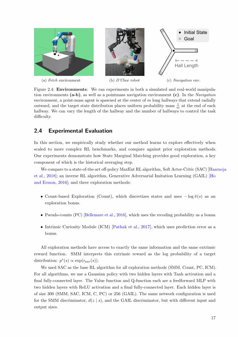
2.4 Environments: We ran experiments in both a simulated and real-world manipu-

lation environments (a-b), as well as a pointmass navigation environment (c). In

the Navigation environment, a point-mass agent is spawned at the center of m long

hallways that extend radially outward, and the target state distribution places uniform

probability mass 1m at the end of each hallway. We can vary the length of the hallway

and the number of hallways to control the task difficulty. . . . . . . . . . . . . . . . 17

2.5 After training, we visualize the policy’s log state marginal over the object coordinates

in Fetch. SMM achieves wider state coverage than baselines. . . . . . . . . . . . . . 19

2.6 The Exploration of SMM: (a) In the Fetch environment, we plot the policy’s

state entropy over the object and gripper coordinates, averaged over 1,000 epochs.

SMM explores more than baselines, as indicated by the larger state entropy (larger

is better). (b) In the D’Claw environment, we trained policies in simulation and

then observed how far the trained policy rotated the knob on the hardware robot,

measuring both the total number of rotations and the minimum and maximum valve

rotations. SMM turns the knob further to the left and right than the baselines, and

also completes a larger cumulative number of rotations. . . . . . . . . . . . . . . . . 20

2.7 Training on Hardware (D’Claw): We trained SAC and SMM on the real robot

for 1e5 environment steps (about 9 hours in real time), and measured the angle turned

throughout training. We see that SMM moves the knob more and visits a wider range

of states than SAC. All results are averaged over 4-5 seeds. . . . . . . . . . . . . . . 20

2.8 Fast Adaptation: (a) We plot the percentage of test-time goals found within

N episodes. SMM and its mixture-model variant SM4 both explore faster than

the baselines, allowing it to successfully find the goal in fewer episodes. (b) We

compare SMM/SM4 with different numbers of mixtures, and with vs. without

historical averaging. Increasing the number of latent mixture components n ∈ {1, 2, 4}accelerates exploration, as does historical averaging. Error bars show std. dev. across

4 random seeds. . . . . . . . . . . . . . . . . . . . . . . . . . . . . . . . . . . . . . . . 21

vi

2.9 Exploration in State Space (SMM) vs. Action Space (SAC) for Navi-

gation : (a) A heatmap showing states visited by SAC and SMM during training

illustrates that SMM explores a wider range of states. (b) SMM reaches more goals

than the MaxEnt baseline. SM4 is an extension of SMM that incorporates mixture

modelling with n > 1 skills (see Appendix 2.1.3), and further improves exploration of

SMM. (c) Ablation Analysis of SM4. On the Navigation task, we compare SM4

(with three mixture components) against ablation baselines that lack conditional state

entropy, latent conditional action entropy, or both (i.e., SAC) in the SM4 objective

(Eq. 2.3). We see that both terms contribute heavily to the exploration ability of

SM4, but the state entropy term is especially critical. . . . . . . . . . . . . . . . . . 22

2.10 With vs. Without Historical Averaging: After training, we rollout the policy

for 1e3 epochs, and record the entropy of the object and gripper positions in Fetch.

SMM achieves higher state entropy than the other methods. Historical averaging also

helps previous exploration methods achieve greater state coverage. . . . . . . . . . . 22

2.11 Non-Uniform Exploration: We measure the discrepancy between the state marginal

distribution, ρπ(s), and a non-uniform target distribution. SMM matches the target

distribution better than SAC and is on par with Count. Error bars show std. dev.

across 4 random seeds. . . . . . . . . . . . . . . . . . . . . . . . . . . . . . . . . . . 23

2.12 SM4 with Eight Mixture Components. In Fetch, we plot the log state marginal

log ρπz(s) over block XY-coordinates for each latent component z ∈ {0, . . . , 7}, results

are averaged over 1000 epochs. . . . . . . . . . . . . . . . . . . . . . . . . . . . . . . 23

3.1 We propose weak supervision as a means to scalably introduce structure into goal-

conditioned RL. The weak supervision is provided by a human who answers true/false

questions (right) based on the two images (left). . . . . . . . . . . . . . . . . . . . . 30

3.2 Our method uses weak supervision, like that depicted in this figure, to direct explo-

ration and accelerate learning on visual manipulation tasks of varying complexity.

Each data sample consists of a pair of image observations {s1, s2} and a factor label

vector y ∈ {0, 1}K , where yk = 1(fk(s1) < fk(s2)) indicates whether the kth factor

of image s1 has smaller value than that of image s2. Example factors of variation

include the gripper position, object positions, brightness, and door angle. Note that

we only need to collect labels for the axes of variation that may be relevant for future

downstream tasks (see Appendix 3.4.5). In environments with ‘light’ as a factor (e.g.,

PushLights), the lighting conditions change randomly at the start of each episode. In

environments with ‘color’ as a factor (e.g., PickupColors), both the object color and

table color randomly change at the start of each episode. Bolded factors correspond

to the user-specified factor indices I indicating which of the factors are relevant for

solving the class of tasks (see Sec. 3.2) . . . . . . . . . . . . . . . . . . . . . . . . . . 31

vii

3.3 Weakly-Supervised Control framework. Left : In Phase 1, we use the weakly-

labelled dataset D = {(s1, s2, y)} to learn a disentangled representation by optimizing

the losses in Eq. 3.1. Right : In Phase 2, we use the learned disentangled representation

to guide goal generation and define distances. At the start of each episode, the agent

samples a latent goal zg either by encoding a goal image g sampled from the replay

buffer, or by sampling directly from the latent goal distribution (Eq. 3.2). The agent

samples actions using the goal-conditioned policy, and defines rewards as the negative

`2 distance between goals and states in the disentangled latent space (Eq. 3.3). . . . 33

3.4 Performance vs. training steps on visual goal-conditioned tasks. Weakly-

Supervised Control (WSC) learns more quickly than prior state-of-the-art goal-

conditioned RL methods (HER, RIG, SkewFit), particularly as the complexity of the

environment grows. Thus, we see that doing directed exploration and goal sampling

in a (learned) semantically-disentangled latent space can be more effective than doing

purely unsupervised exploration in the VAE latent space. . . . . . . . . . . . . . . . 36

3.5 We roll out trained policies on visual goal-conditioned tasks, and compare the latent

goal distance vs. the true goal distance between the object and the goal position. As

the environment becomes increasingly complex (Push with n ∈ {1, 2, 3} objects), the

latent distance reward optimized by SkewFit becomes less indicative of the true goal

distance, whereas the disentangled distance optimized by our method remains more

accurate. . . . . . . . . . . . . . . . . . . . . . . . . . . . . . . . . . . . . . . . . . . 37

3.6 SkewFit+DR is a variant that samples goals in VAE latent space, but uses reward

distances in disentangled latent space. We see that the disentangled distance metric

can help slightly in harder environments (e.g., Push n = 3), but the goal generation

mechanism of WSC is crucial to achieving efficient exploration. . . . . . . . . . . . . 38

3.7 Interpretable control: Trajectories generated by WSC (left) and SkewFit (right),

where the policies are conditioned on varying latent goals (z1, z2) ∈ R2. For SkewFit,

we varied the latent dimensions that have the highest correlation with the object’s

XY-position, and kept the remaining latent dimensions fixed. The blue object always

starts at the center of the frame in the beginning of each episode. The white lines

indicate the target object’s position throughout the trajectory. We see that the

disentangled latent goal values of WSC directly align with the direction in which the

WSC policy moves the blue object. . . . . . . . . . . . . . . . . . . . . . . . . . . . 45

3.8 How many factors of variation need to be labelled? WSC outperforms SkewFit

even without being provided weak labels for task-irrelevant factors, such as hand

position and lighting. . . . . . . . . . . . . . . . . . . . . . . . . . . . . . . . . . . . . 46

3.9 How many weak labels are needed to help visual goal-conditioned RL? We

evaluate the performance of our method (WSC) on visual goal-conditioned tasks as

we vary the number of weak pairwise labels N ∈ {128, 256, . . . , 4096}. We find that

1024 pairwise labels is generally sufficient for good performance on all domains. . . 46

viii

3.10 Real-world dataset: (a): We collected 1,285 RGB camera images (1,029 train,

256 test) on a real Franka robot with 5 block objects, and then had a human provide

weak labels for the block positions. We collected the images under various lighting

conditions, and used two camera viewpoints to overcome object occlusion. (b): Our

method attains a sufficiently high Pearson correlation between the true XY-position

of the block (relative to the image frame) vs. the latent dimension of the encoded

image, suggesting that weakly-supervised disentangled representation learning may

be useful for training robots in the real-world. Results are taken over 6 seeds. . . . 46

4.1 (a) We consider embodied multimodal tasks, where the agent receives visual first-

person observations and an instruction or a question specifying the task. (b) Example

starting states and bird’s eye view of the map showing agent and candidate object

locations in Easy and Hard settings. . . . . . . . . . . . . . . . . . . . . . . . . . . . 49

4.2 Overview of our proposed architecture, described in detail in Section 4.3. . . . . . . 51

4.3 The Dual-Attention unit uses two types of attention mechanisms (a, b) to align

representations in different modalities and tasks. . . . . . . . . . . . . . . . . . . . . 52

4.4 Architecture of the Dual-Attention unit with example intermediate representations

and operations. . . . . . . . . . . . . . . . . . . . . . . . . . . . . . . . . . . . . . . . 53

4.5 Example auxiliary task labels for the red channel. . . . . . . . . . . . . . . . . . . . 55

4.6 Training accuracy of all models trained with auxiliary tasks for Easy (left) and Hard

(right). . . . . . . . . . . . . . . . . . . . . . . . . . . . . . . . . . . . . . . . . . . . . 55

4.7 Training accuracy of all models trained without auxiliary tasks for Easy (left) and

Hard (right). . . . . . . . . . . . . . . . . . . . . . . . . . . . . . . . . . . . . . . . . 56

4.8 Visualizations of convolutional output channels. We visualize the convolutional

channels corresponding to 7 words (one in each row) for the same frame (shown in the

rightmost column). The first column shows the auxiliary task labels for reference. The

second column and third column show the output of the corresponding channel for the

proposed Dual-Attention model trained without and with auxiliary tasks, respectively.

As expected, the Aux model outputs are very close to the auxiliary task labels. The

convolutional outputs of the No Aux model show that words and objects/properties

in the images have been properly aligned even when the model is not trained with

any auxiliary task labels. We do not provide any auxiliary label for words ‘smallest’

and ‘largest’ as they are not properties of an object and require relative comparison

of objects. The visualizations in row 5 (corresponding to ‘smallest’) indicate that

both models are able to compare the sizes of objects and detect the smallest object in

the corresponding output channel even without any aux labels for the smallest object. 58

ix

4.9 Spatial Attention and Answer Prediction Visualizations. An example EQA

episode with the question “Which is the smallest blue object?”. The sentence

embedding of the question is shown on the top (xsent). As expected, the embedding

attends to object type words (’torch’, ’pillar’, ’skullkey’, etc.) as the question is asking

about an object type (’Which object’). The rows show increasing time steps and

columns show the input frame, the input frame overlaid with the spatial attention

map, the predicted answer distribution, and the action at each time step. As the

agent is turning, the spatial attention attends to small and blue objects. Time steps

1, 2: The model is attending to the yellow skullkey but the probability of the answer

is not sufficiently high, likely because the skullkey is not blue. Time step 3: The

model cannot see the skullkey anymore so it attends to the armor which is next

smallest object. Consequently, the answer prediction also predicts armor, but the

policy decides not to answer due to low probability. Time step 4: As the agent

turns more, it observes and attends to the blue skullkey. The answer prediction for

‘skullkey’ has high probability because it is small and blue, so the policy decides to

answer the question. . . . . . . . . . . . . . . . . . . . . . . . . . . . . . . . . . . . 59

4.10 Training accuracy of proposed Dual-Attention model with all ablation models trained

without (left) and with (right) auxiliary tasks for the Easy environment. . . . . . . . 60

List of Tables

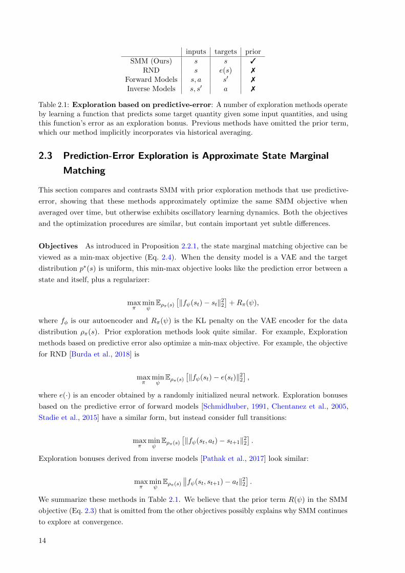
2.1 Exploration based on predictive-error: A number of exploration methods op-

erate by learning a function that predicts some target quantity given some input

quantities, and using this function’s error as an exploration bonus. Previous methods

have omitted the prior term, which our method implicitly incorporates via historical

averaging. . . . . . . . . . . . . . . . . . . . . . . . . . . . . . . . . . . . . . . . . . 14

3.1 Conceptual comparison between our method weakly-supervised control (WSC), and

prior visual goal-conditioned RL methods, with their respective latent goal distribu-

tions p(Z) and goal-conditioned reward functions Rzg(s′). Our method can be seen

as an extension of prior work to the weakly-supervised setting. . . . . . . . . . . . . 35

x

3.2 Is the learned state representation disentangled? We measure the correlation

between the true factor value of the input image vs. the latent dimension of the

encoded image on the evaluation dataset. We show the 95% confidence interval

over 5 seeds. We find that unsupervised VAEs are often insufficient for learning a

disentangled representation. . . . . . . . . . . . . . . . . . . . . . . . . . . . . . . . 39

3.3 Is the learned policy interpretable? We investigate whether latent goals zg align

directly with the final state of the trajectory after rolling out π(a | s, zg). We measure

the correlation between the true factor value of the final state in the trajectory vs.

the corresponding latent dimension of zg. We show the 95% confidence interval over

5 seeds. Our method attains higher correlation between latent goals and final states,

meaning that it learns a more interpretable goal-conditioned policy. . . . . . . . . . 40

3.4 How many weak labels are needed to learn a sufficiently-disentangled state

representation? We trained disentangled representations on varying numbers of

weakly-labelled data samples {(s(i)1 , s

(i)2 , y(i))}Ni=1 (N ∈ {128, 256, . . . , 4096}), then

evaluated how well they disentangled the true factors of variation in the data. On

the evaluation dataset, we measure the Pearson correlation between the true factor

value of the input image vs. the latent dimension of the encoded image. For the

VAE (obtained from SkewFit), we took the latent dimension that has the highest

correlation with the true factor value. We report the 95% confidence interval over 5

seeds. Even with a small amount of weak supervision (e.g. around 1024 labels), we

are able to attain a representation with good disentanglement. . . . . . . . . . . . . 41

3.5 Noisy labels: We trained disentangled representations on noisy PushLights datasets

for n ∈ {1, 2, 3} objects, where each factor label was corrupted with probability 5%

or 10%. We then measured the Pearson correlation between the true factor values vs.

the corresponding latent dimension. Our method learns robustly-disentangled repre-

sentations with 5% noise (around 80% correlation), but achieves lower performance

with 10% noise (around 60-70% correlation). Results are taken over 5 seeds. . . . . 41

4.1 Table showing training and test sets for both Semantic Goal Navigation (SGN)

and Embodied Question Answering (EQA) tasks. The test set consists of unseen

instructions and questions. The dataset evaluates a model for cross-task knowledge

transfer between SGN and EQA. . . . . . . . . . . . . . . . . . . . . . . . . . . . . . 50

4.2 Accuracy of all models on SGN & EQA test sets for both Easy & Hard difficulties. 57

4.3 Accuracy of all the ablation models trained with and without Auxiliary tasks on SGN

and EQA test sets for the Doom Easy environment. . . . . . . . . . . . . . . . . . . 60

4.4 The performance of a trained policy appended with object detectors on instructions

containing unseen words (‘red’ and ‘pillar’). . . . . . . . . . . . . . . . . . . . . . . . 60

A.1 Environment parameters specifying the observation space dimension |S|; action

space dimension |A|; max episode length T ; the environment reward, related to the

target distribution by exp{renv(s)} ∝ p∗(s), and other environment parameters. . . . 68

xi

A.2 Hyperparameter settings. Hyperparameters were chosen according to the following eval metrics:

Fetch-Uniform: State entropy of the discretized gripper and block positions (bin size 0.05), after

rolling out the trained policy for 50K env steps. Fetch-Half : DKL(p∗(s) ‖ ρπ(s)) and TV(p∗(s), ρπ(s))

of the discretized gripper and block positions (bin size 0.01), after rolling out the trained policy for

50K env steps. 2D Navigation: State entropy of the discretized XY-positions of the trained policy.

D’Claw : State entropy of the object angle. . . . . . . . . . . . . . . . . . . . . . . . . . . . 70

A.3 Environment-specific hyperparameters: M is the number of training images.

“WSC pgoal” is the percentage of relabelled goals in WSC (Alg. 3). αDR is the VAE

reward coefficient for SkewFit+DR in Eq. A.1. . . . . . . . . . . . . . . . . . . . . . 71

A.4 Disentangled representation model architecture: We slightly modified the

disentangled model architecture from Shu et al. [2019] for 48× 48 image observations.

The discriminator body is applied separately to s1 and s2 to compute the unconditional

logits o1 and o2 respectively, and the conditional logit is computed as odiff = y·(h1−h2),

where h1, h2 are the hidden layers and y ∈ {±1}. . . . . . . . . . . . . . . . . . . . . 71

A.5 VAE architecture & hyperparameters: β is the KL regularization coefficient in

the β-VAE loss. We found that a smaller VAE latent dim LVAE ∈ {4, 16} worked

best for SkewFit, RIG, and HER (which use the VAE for both hindsight relabelling

and for the actor & critic networks), but a larger dim LVAE = 256 benefitted WSC

(which only uses the VAE for the actor & critic networks). . . . . . . . . . . . . . . 71

xii

Chapter 1

Introduction

Reinforcement learning (RL) is a field within machine learning which studies how an agent learns to

perform a task through trial-and-error interactions with an initially unknown environment. Deep

learning has helped achieve major breakthroughs in RL by enabling methods to automatically

learn features from high-dimensional observations, such as image pixels, tactile sensors, and

robot joint sensors. As a result, these advances have especially benefited robotic and vision-based

applications, enabling RL agents to solve specific, well-defined tasks from low-level sensory inputs.

Despite the progress, several unsolved challenges limit the applicability of RL to real world

tasks. RL is computationally intensive to train, especially in domains where each interaction with

the environment is expensive. Real world applications require the agent to solve a wide variety

of tasks, but training RL from scratch for each task is computationally infeasible. It remains an

open challenge to improve the learning and data efficiency of RL agents, and to share and reuse

experience across tasks so that learned skills can be transferred to new tasks and dynamics.

Most importantly, the cost of human supervision is perhaps the largest roadblock for widely

deploying RL in the real world. Reward functions require inordinate amounts of tuning and

can be difficult to design, especially in high-dimensional problems. Instead of relying on reward

functions, an alternative approach is to learn to imitate some expert behavior. However, these

imitation learning approaches, such as inverse RL [Hadfield-Menell et al., 2017, Ziebart et al.,

2008, Fu et al., 2017], have a voracious appetite for expert demonstrations, which can be difficult

to obtain in domains with high-dimensional action spaces. Moreover, human demonstrations are

often not perfect, and it remains an open question of how to explore and extrapolate beyond

suboptimal demonstrations [Levine, 2018, Brown et al., 2019].

To reduce data requirements for RL, there has been recent progress on self-supervised RL

approaches, where the agent learns on its own by interacting with the environment. These

include intrinsic rewards for exploration [Burda et al., 2018, Schmidhuber, 1991, Chentanez et al.,

2005, Stadie et al., 2015, Pathak et al., 2017], mutual-information objectives [Achiam et al.,

2018, Eysenbach et al., 2018, Co-Reyes et al., 2018], and goal-conditioned RL [Andrychowicz

et al., 2017] among others. While these methods do not require an extrinsic reward function

or demonstration provided by a human, self-supervised approaches are notorious for being

sample-inefficient and computationally expensive to train.

Can we find a balance between self-supervision and human-supervision for training RL

algorithms? In this thesis, we will be mindful about the cost of human supervision, and consider

1

alternative modalities of supervision that can be more scalable and easier to provide from the

human. When thinking about how to scalably supervise RL, there are a number of desiderata to

consider:

1. Convenient user interface: A human should be able to supervise and interact with the

agent in a way that is easy and accessible to anyone, without requiring much time or expert

knowledge. The user interface should also support multimodal supervision signals, allowing

the human to provide different modalities of feedback (e.g., verbal language instructions

and visual cues).

2. Data-efficient learning : The algorithm should be sample-efficient with respect to both the

number of environment interactions, as well as the number of human labels. We should be

conscious of how much time the human needs to spend supervising the agent, and we should

also utilize that supervision in order to drastically cut down the number of environment

interactions needed.

3. Efficient, safe, and controllable exploration: In order to achieve effective and efficient

human-agent interaction, the agent needs to have efficient exploration capabilities. In other

words, the agent should be equipped with the ability to explore interesting and novel states,

so that the human can provide feedback on a diverse range of behaviors. The agent should

also be able to explore in a safe and controllable manner, so that the agent can learn on its

own without requiring constant supervision.

With all of these points in mind, we will study how we can balance self-supervised RL with

scalable forms of human supervision in order to accelerate learning, improve generalization, and

amortize the cost of human supervision. We will show how scalable supervision can be used to

greatly benefit exploration and representation learning for RL, significantly improving learning

efficiency over purely self-supervised approaches, while being less costly than fully-supervised

approaches.

1.1 Overview

Chapter 2: Task-Agnostic Exploration via State Marginal Matching

Having a good exploratory policy that visits a diverse range of states can enable the agent to

learn faster, especially in sparse reward settings, and also allows the human to provide more

meaningful feedback on the agent’s behavior. Moreover, being able to control how the agent

does exploration can improve safety for deploying RL algorithms in real-world scenarios, and

accelerate learning by focusing training on only the relevant subspace of tasks.

There has been considerable progress on exploration for RL, one common approach being

intrinsic rewards as exploration bonuses [Burda et al., 2018, Schmidhuber, 1991, Chentanez et al.,

2005, Stadie et al., 2015, Pathak et al., 2017]. However, these methods are often focused on

learning to explore for only a single task, and it is unclear how to repurpose these methods for

multi-task exploration, i.e., reusing exploration experience from one task to acquire exploration

strategies for another task. Moreover, it is often unclear what underlying objective is being

2

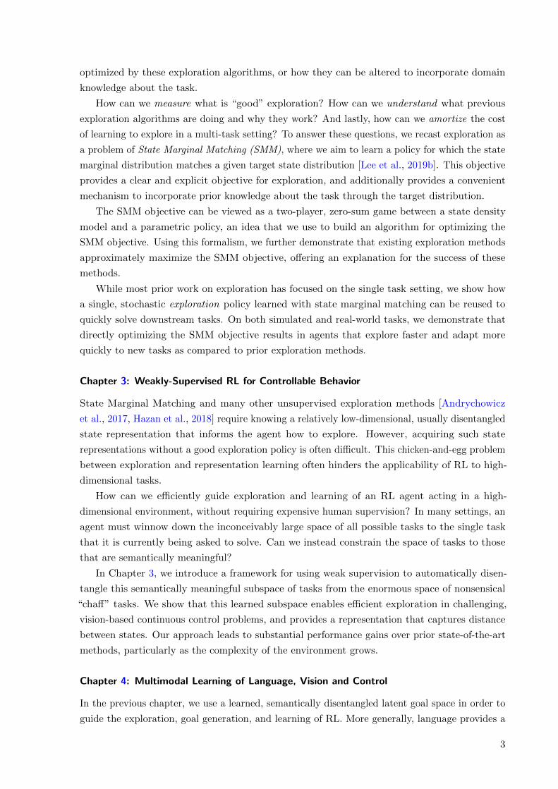
optimized by these exploration algorithms, or how they can be altered to incorporate domain

knowledge about the task.

How can we measure what is “good” exploration? How can we understand what previous

exploration algorithms are doing and why they work? And lastly, how can we amortize the cost

of learning to explore in a multi-task setting? To answer these questions, we recast exploration as

a problem of State Marginal Matching (SMM), where we aim to learn a policy for which the state

marginal distribution matches a given target state distribution [Lee et al., 2019b]. This objective

provides a clear and explicit objective for exploration, and additionally provides a convenient

mechanism to incorporate prior knowledge about the task through the target distribution.

The SMM objective can be viewed as a two-player, zero-sum game between a state density

model and a parametric policy, an idea that we use to build an algorithm for optimizing the

SMM objective. Using this formalism, we further demonstrate that existing exploration methods

approximately maximize the SMM objective, offering an explanation for the success of these

methods.

While most prior work on exploration has focused on the single task setting, we show how

a single, stochastic exploration policy learned with state marginal matching can be reused to

quickly solve downstream tasks. On both simulated and real-world tasks, we demonstrate that

directly optimizing the SMM objective results in agents that explore faster and adapt more

quickly to new tasks as compared to prior exploration methods.

Chapter 3: Weakly-Supervised RL for Controllable Behavior

State Marginal Matching and many other unsupervised exploration methods [Andrychowicz

et al., 2017, Hazan et al., 2018] require knowing a relatively low-dimensional, usually disentangled

state representation that informs the agent how to explore. However, acquiring such state

representations without a good exploration policy is often difficult. This chicken-and-egg problem

between exploration and representation learning often hinders the applicability of RL to high-

dimensional tasks.

How can we efficiently guide exploration and learning of an RL agent acting in a high-

dimensional environment, without requiring expensive human supervision? In many settings, an

agent must winnow down the inconceivably large space of all possible tasks to the single task

that it is currently being asked to solve. Can we instead constrain the space of tasks to those

that are semantically meaningful?

In Chapter 3, we introduce a framework for using weak supervision to automatically disen-

tangle this semantically meaningful subspace of tasks from the enormous space of nonsensical

“chaff” tasks. We show that this learned subspace enables efficient exploration in challenging,

vision-based continuous control problems, and provides a representation that captures distance

between states. Our approach leads to substantial performance gains over prior state-of-the-art

methods, particularly as the complexity of the environment grows.

Chapter 4: Multimodal Learning of Language, Vision and Control

In the previous chapter, we use a learned, semantically disentangled latent goal space in order to

guide the exploration, goal generation, and learning of RL. More generally, language provides a

3

way to encode combinatorial abstractions and generalizations of the visual and physical world.

It also enables us to communicate instructions, questions, plans, and intentions to one another.

How can we utilize language to equip deep RL agents with structured priors about the physical

world, and enable generalization and knowledge transfer across different tasks?

As a case study, we consider training an embodied agent with goals specified via language.

The embodied agent interacts with a 3D environment by receiving first-person RGB views of the

environment and taking navigational actions. We introduce a dual-attention architecture that

disentangles the knowledge of words and visual attributes in order to transfer grounded knowledge

across different tasks, and to new words and concepts not seen during training [Chaplot et al.,

2020]. Additionally, we demonstrate that the modularity of our model allows easy addition of

new objects and attributes to a trained model.

1.2 Summary of Publications & Open-Source Contributions

The content of chapter 2 appears in:

Lisa Lee, Benjamin Eysenbach, Emilio Parisotto, Eric Xing, Sergey Levine, and

Ruslan Salakhutdinov. Efficient exploration via state marginal matching. arXiv

preprint arXiv:1906.05274, 2019b

Code: https://github.com/RLAgent/state-marginal-matching

The content of chapter 3 appears in:

Lisa Lee, Benjamin Eysenbach, Ruslan Salakhutdinov, Chelsea Finn, et al. Weakly-

supervised reinforcement learning for controllable behavior. Neural Information

Processing Systems (NeurIPS), 2020

Code: https://github.com/google-research/weakly_supervised_control

The content of chapter 4 appears in:

Devendra Singh Chaplot, Lisa Lee, Ruslan Salakhutdinov, Devi Parikh, and Dhruv

Batra. Embodied multimodal multitask learning. International Joint Conference

on Artificial Intelligence (IJCAI), 2020

Code: https://github.com/devendrachaplot/DeepRL-Grounding

I have also pursued the following research directions during my Ph.D. studies, which are excluded

from this thesis:

Lisa Lee, Emilio Parisotto, Devendra Singh Chaplot, Eric Xing, and Ruslan

Salakhutdinov. Gated path planning networks. In International Conference on

4

Machine Learning (ICML), pages 2947–2955. PMLR, 2018

Code: https://github.com/RLAgent/gated-path-planning-networks

Tianwei Ni, Harshit Sikchi, Yufei Wang, Tejus Gupta, Lisa Lee, and Benjamin

Eysenbach. F-irl: Inverse reinforcement learning via state marginal matching.

Conference on Robot Learning (CoRL), 2020

Code: https://github.com/twni2016/f-IRL

Xiaodan Liang, Lisa Lee, and Eric P Xing. Deep variation-structured reinforcement

learning for visual relationship and attribute detection. In Proceedings of the IEEE

conference on Computer Vision and Pattern Recognition (CVPR), pages 848–857,

2017b

Xiaodan Liang, Lisa Lee, Wei Dai, and Eric P Xing. Dual motion gan for future-flow

embedded video prediction. In Proceedings of the IEEE International Conference

on Computer Vision (ICCV), pages 1744–1752, 2017a

Yohan Jo, Lisa Lee, and Shruti Palaskar. Combining lstm and latent topic modeling

for mortality prediction. arXiv preprint arXiv:1709.02842, 2017

Maruan Al-Shedivat, Lisa Lee, Ruslan Salakhutdinov, and Eric Xing. On the com-

plexity of exploration in goal-driven navigation. arXiv preprint arXiv:1811.06889,

2018

5

Chapter 2

Task-Agnostic Exploration via

State Marginal Matching

Reinforcement learning (RL) algorithms must be equipped with exploration mechanisms to

effectively solve tasks with long horizons and limited or delayed reward signals. These tasks arise

in many real-world applications where providing human supervision is expensive.

Exploration for RL has been studied in a wealth of prior work. The optimal exploration

strategy is intractable to compute in most settings, motivating work on tractable heuristics

for exploration [Kolter and Ng, 2009]. Exploration methods based on random actions have

limited ability to cover a wide range of states. More sophisticated techniques, such as intrinsic

motivation, accelerate learning in the single-task setting. However, these methods have two

limitations: (1) First, they lack an explicit objective to quantify “good exploration,” but rather

argue that exploration arises implicitly through some iterative procedure. Lacking a well-defined

optimization objective, it remains unclear what these methods are doing and why they work.

Similarly, the lack of a metric to quantify exploration, even if only for evaluation, makes it difficult

to compare exploration methods and assess progress in this area. (2) The second limitation is

that these methods target the single-task setting. Because these methods aim to converge to the

optimal policy for a particular task, it is difficult to repurpose these methods to solve multiple

tasks.

We address these shortcomings by recasting exploration as a problem of State Marginal

Matching (SMM): Given a target state distribution, we learn a policy for which the state marginal

distribution matches this target distribution. Not only does the SMM problem provide a clear

and explicit objective for exploration, but it also provides a convenient mechanism to incorporate

prior knowledge about the task through the target distribution — whether in the form of safety

constraints that the agent should obey; preferences for some states over other states; reward

shaping; or the relative importance of each state dimension for a particular task. Without any

prior information, the SMM objective reduces to maximizing the marginal state entropy H[s],

which encourages the policy to visit all states.

In this work, we study state marginal matching as a metric for task-agnostic exploration.

While this class of objectives has been considered in Hazan et al. [2018], we build on this prior

work in a number of dimensions:

7

1. We argue that the SMM objective is an effective way to learn a single, task-agnostic

exploration policy that can be used for solving many downstream tasks, amortizing the cost

of learning to explore for each task. Learning a single exploration policy is considerably

more difficult than doing exploration throughout the course of learning a single task. The

latter is done by intrinsic motivation [Pathak et al., 2017, Tang et al., 2017, Oudeyer et al.,

2007] and count-based exploration [Bellemare et al., 2016], which can effectively explore

to find states with high reward, at which point the agent can decrease exploration and

increase exploitation of those high-reward states. While these methods perform efficient

exploration for learning a single task, we show in Sec. 2.3 that the policy at any particular

iteration is not a good exploration policy.

In contrast, maximizing H[s] produces a stochastic policy at convergence that visits states in

proportion to their density under a target distribution. We use this policy as an exploration

prior in our multi-task experiments, and also prove that this policy is optimal for a class of

goal-reaching tasks (Section 2.5).

2. We explain how to optimize the SMM objective properly. By viewing the objective as

a two-player, zero-sum game between a state density model and a parametric policy, we

propose a practical algorithm to jointly learn the policy and the density by using fictitious

play [Brown, 1951].

We further decompose the SMM objective into a mixture of distributions, and derive

an algorithm for learning a mixture of policies that resembles the mutual-information

objectives in recent work [Achiam et al., 2018, Eysenbach et al., 2018, Co-Reyes et al., 2018].

Thus, these prior work may be interpreted as also almost doing distribution matching, with

the caveat that they omit the state entropy term.

3. Our analysis provides a unifying view of prior exploration methods as almost performing

distribution matching. We show that exploration methods based on predictive error

approximately optimizes the same SMM objective, offering an explanation for the success

of these methods. However, they omit a crucial historical averaging step, potentially

explaining why they do not converge to an exploratory policy.

4. We demonstrate on complex RL tasks that optimizing the SMM objective allows for faster

exploration and adaptation than prior state-of-the-art exploration methods.

In short, our work contributes a method to measure, amortize, and understand exploration.

2.1 State Marginal Matching

In this section, we start by showing that exploration methods based on prediction error do not

acquire a single exploratory policy. This motivates us to define the State Marginal Matching

problem as a principled objective for learning to explore. We then introduce an extension of the

SMM objective using a mixture of policies.

8

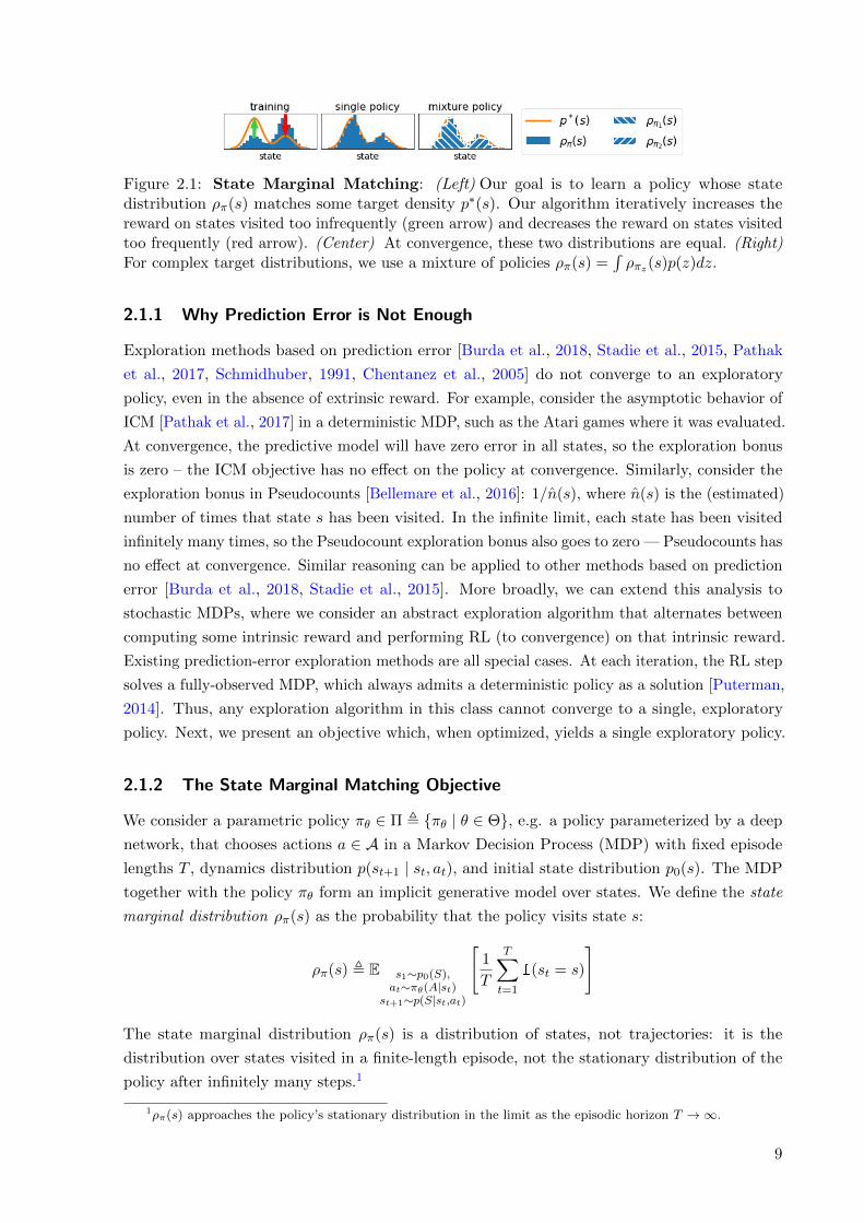
Figure 2.1: State Marginal Matching: (Left) Our goal is to learn a policy whose statedistribution ρπ(s) matches some target density p∗(s). Our algorithm iteratively increases thereward on states visited too infrequently (green arrow) and decreases the reward on states visitedtoo frequently (red arrow). (Center) At convergence, these two distributions are equal. (Right)For complex target distributions, we use a mixture of policies ρπ(s) =

∫ρπz(s)p(z)dz.

2.1.1 Why Prediction Error is Not Enough

Exploration methods based on prediction error [Burda et al., 2018, Stadie et al., 2015, Pathak

et al., 2017, Schmidhuber, 1991, Chentanez et al., 2005] do not converge to an exploratory

policy, even in the absence of extrinsic reward. For example, consider the asymptotic behavior of

ICM [Pathak et al., 2017] in a deterministic MDP, such as the Atari games where it was evaluated.

At convergence, the predictive model will have zero error in all states, so the exploration bonus

is zero – the ICM objective has no effect on the policy at convergence. Similarly, consider the

exploration bonus in Pseudocounts [Bellemare et al., 2016]: 1/n(s), where n(s) is the (estimated)

number of times that state s has been visited. In the infinite limit, each state has been visited

infinitely many times, so the Pseudocount exploration bonus also goes to zero — Pseudocounts has

no effect at convergence. Similar reasoning can be applied to other methods based on prediction

error [Burda et al., 2018, Stadie et al., 2015]. More broadly, we can extend this analysis to

stochastic MDPs, where we consider an abstract exploration algorithm that alternates between

computing some intrinsic reward and performing RL (to convergence) on that intrinsic reward.

Existing prediction-error exploration methods are all special cases. At each iteration, the RL step

solves a fully-observed MDP, which always admits a deterministic policy as a solution [Puterman,

2014]. Thus, any exploration algorithm in this class cannot converge to a single, exploratory

policy. Next, we present an objective which, when optimized, yields a single exploratory policy.

2.1.2 The State Marginal Matching Objective

We consider a parametric policy πθ ∈ Π , {πθ | θ ∈ Θ}, e.g. a policy parameterized by a deep

network, that chooses actions a ∈ A in a Markov Decision Process (MDP) with fixed episode

lengths T , dynamics distribution p(st+1 | st, at), and initial state distribution p0(s). The MDP

together with the policy πθ form an implicit generative model over states. We define the state

marginal distribution ρπ(s) as the probability that the policy visits state s:

ρπ(s) , E s1∼p0(S),at∼πθ(A|st)

st+1∼p(S|st,at)

[1

T

T∑t=1

1(st = s)

]

The state marginal distribution ρπ(s) is a distribution of states, not trajectories: it is the

distribution over states visited in a finite-length episode, not the stationary distribution of the

policy after infinitely many steps.1

1ρπ(s) approaches the policy’s stationary distribution in the limit as the episodic horizon T → ∞.

9

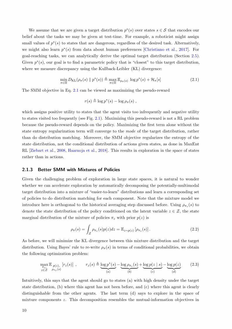
We assume that we are given a target distribution p∗(s) over states s ∈ S that encodes our

belief about the tasks we may be given at test-time. For example, a roboticist might assign

small values of p∗(s) to states that are dangerous, regardless of the desired task. Alternatively,

we might also learn p∗(s) from data about human preferences [Christiano et al., 2017]. For

goal-reaching tasks, we can analytically derive the optimal target distribution (Section 2.5).

Given p∗(s), our goal is to find a parametric policy that is “closest” to this target distribution,

where we measure discrepancy using the Kullback-Leibler (KL) divergence:

minπ∈Π

DKL(ρπ(s) ‖ p∗(s)) , maxπ∈Π

Eρπ(s) log p∗(s) +Hπ[s] (2.1)

The SMM objective in Eq. 2.1 can be viewed as maximizing the pseudo-reward

r(s) , log p∗(s)− log ρπ(s) ,

which assigns positive utility to states that the agent visits too infrequently and negative utility

to states visited too frequently (see Fig. 2.1). Maximizing this pseudo-reward is not a RL problem

because the pseudo-reward depends on the policy. Maximizing the first term alone without the

state entropy regularization term will converge to the mode of the target distribution, rather

than do distribution matching. Moreover, the SMM objective regularizes the entropy of the

state distribution, not the conditional distribution of actions given states, as done in MaxEnt

RL [Ziebart et al., 2008, Haarnoja et al., 2018]. This results in exploration in the space of states

rather than in actions.

2.1.3 Better SMM with Mixtures of Policies

Given the challenging problem of exploration in large state spaces, it is natural to wonder

whether we can accelerate exploration by automatically decomposing the potentially-multimodal

target distribution into a mixture of “easier-to-learn” distributions and learn a corresponding set

of policies to do distribution matching for each component. Note that the mixture model we

introduce here is orthogonal to the historical averaging step discussed before. Using ρπz(s) to

denote the state distribution of the policy conditioned on the latent variable z ∈ Z, the state

marginal distribution of the mixture of policies πz with prior p(z) is

ρπ(s) =

∫Zρπz(s)p(z)dz = Ez∼p(z) [ρπz(s)] . (2.2)

As before, we will minimize the KL divergence between this mixture distribution and the target

distribution. Using Bayes’ rule to re-write ρπ(s) in terms of conditional probabilities, we obtain

the following optimization problem:

maxπz ,z∈Z

E p(z),ρπz (s)

[rz(s)] , rz(s) , log p∗(s)︸ ︷︷ ︸(a)

− log ρπz(s)︸ ︷︷ ︸(b)

+ log p(z | s)︸ ︷︷ ︸(c)

− log p(z)︸ ︷︷ ︸(d)

(2.3)

Intuitively, this says that the agent should go to states (a) with high density under the target

state distribution, (b) where this agent has not been before, and (c) where this agent is clearly

distinguishable from the other agents. The last term (d) says to explore in the space of

mixture components z. This decomposition resembles the mutual-information objectives in

10

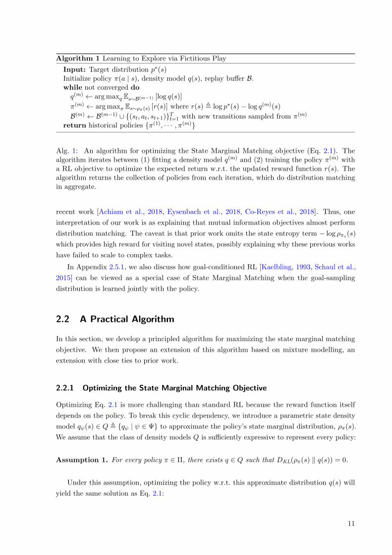
Algorithm 1 Learning to Explore via Fictitious Play

Input: Target distribution p∗(s)Initialize policy π(a | s), density model q(s), replay buffer B.while not converged doq(m) ← arg maxq Es∼B(m−1) [log q(s)]

π(m) ← arg maxπ Es∼ρπ(s) [r(s)] where r(s) , log p∗(s)− log q(m)(s)

B(m) ← B(m−1) ∪ {(st, at, st+1)}Tt=1 with new transitions sampled from π(m)

return historical policies {π(1), · · · , π(m)}

Alg. 1: An algorithm for optimizing the State Marginal Matching objective (Eq. 2.1). Thealgorithm iterates between (1) fitting a density model q(m) and (2) training the policy π(m) witha RL objective to optimize the expected return w.r.t. the updated reward function r(s). Thealgorithm returns the collection of policies from each iteration, which do distribution matchingin aggregate.

recent work [Achiam et al., 2018, Eysenbach et al., 2018, Co-Reyes et al., 2018]. Thus, one

interpretation of our work is as explaining that mutual information objectives almost perform

distribution matching. The caveat is that prior work omits the state entropy term − log ρπz(s)

which provides high reward for visiting novel states, possibly explaining why these previous works

have failed to scale to complex tasks.

In Appendix 2.5.1, we also discuss how goal-conditioned RL [Kaelbling, 1993, Schaul et al.,

2015] can be viewed as a special case of State Marginal Matching when the goal-sampling

distribution is learned jointly with the policy.

2.2 A Practical Algorithm

In this section, we develop a principled algorithm for maximizing the state marginal matching

objective. We then propose an extension of this algorithm based on mixture modelling, an

extension with close ties to prior work.

2.2.1 Optimizing the State Marginal Matching Objective

Optimizing Eq. 2.1 is more challenging than standard RL because the reward function itself

depends on the policy. To break this cyclic dependency, we introduce a parametric state density

model qψ(s) ∈ Q , {qψ | ψ ∈ Ψ} to approximate the policy’s state marginal distribution, ρπ(s).

We assume that the class of density models Q is sufficiently expressive to represent every policy:

Assumption 1. For every policy π ∈ Π, there exists q ∈ Q such that DKL(ρπ(s) ‖ q(s)) = 0.

Under this assumption, optimizing the policy w.r.t. this approximate distribution q(s) will

yield the same solution as Eq. 2.1:

11

Algorithm 2 State Marginal Matching with Mixtures of Mixtures (SM4)

Input: Target distribution p∗(s)Initialize policy πz(a | s), density model qz(s), discriminator d(z | s), and replay buffer B.while not converged do

for z = 1, · · · , n do

q(m)z ← arg maxq E{s|(z′,s)∼B(m−1),z′=z} [log q(s)]

d(m) ← arg maxd E(z,s)∼B(m−1) [log d(z | s)] {(2) Update discriminator.}for z = 1, · · · , n do

r(m)z (s) , log p∗(s)− log q

(m)z (s) + log d(m)(z | s)− log p(z)

π(m)z ← arg maxπ Eρπ(s)

[r

(m)z (s)

]Sample latent skill z(m) ∼ p(z)Sample transitions {(st, at, st+1)}Tt=1 with π

(m)z (a | s)

B(m) ← B(m−1) ∪ {(z(m), st, at, st+1)}Tt=1

return {{π(1)1 , · · · , π(1)

n }, · · · , {π(m)1 , · · · , π(m)

n }}

Alg. 2: An algorithm for learning a mixture of policies π1, π2, · · · , πn that do state marginal

matching in aggregate. The algorithm (1) fits a density model q(m)z (s) to approximate the state

marginal distribution for each policy πz; (2) learns a discriminator d(m)(z | s) to predict whichpolicy πz will visit state s; and (3) uses RL to update each policy πz to maximize the expectedreturn of its corresponding reward function derived in Eq. 2.3. In our implementation, the densitymodel qz(s) is a VAE that inputs the concatenated vector {s, z} of the state s and the latentskill z used to obtain this sample s; and the discriminator is a feedforward MLP. The algorithmreturns the historical average of mixtures of policies (a total of n ·m policies).

Proposition 2.2.1. Let policies Π and density models Q satisfying Assumption 1 be given. For

any target distribution p∗, the following optimization problems are equivalent:

maxπ

Eρπ(s)[log p∗(s)− log ρπ(s)] = maxπ

minq

Eρπ(s)[log p∗(s)− log q(s)] (2.4)

Proof of Proposition 2.2.1. Note that the objective in Eq. 2.4 can be written as

Eρπ(s)[log p∗(s)− log ρπ(s)] +DKL(ρπ(s) ‖ q(s)).

By Assumption 1, DKL(ρπ(s) ‖ q(s)) = 0 for some q ∈ Q, so we obtain the desired result:

maxπ

(minq

Eρπ(s)[log p∗(s)− log q(s)]

)= max

π

(Eρπ(s)[log p∗(s)− log ρπ(s)] + min

qDKL(ρπ(s) ‖ q(s))

)= max

πEρπ(s)[log p∗(s)− log ρπ(s)].

Solving the new max-min optimization problem is equivalent to finding the Nash equilibrium

of a two-player, zero-sum game: a policy player chooses the policy π while the density player

chooses the density model q. To avoid confusion, we use actions to refer to controls a ∈ A output

by the policy π in the traditional RL problem and strategies to refer to the decisions of the policy

player π ∈ Π and density player q ∈ Q. The Nash existence theorem [Nash, 1951] proves that

such a stationary point always exists for such a two-player, zero-sum game.

12

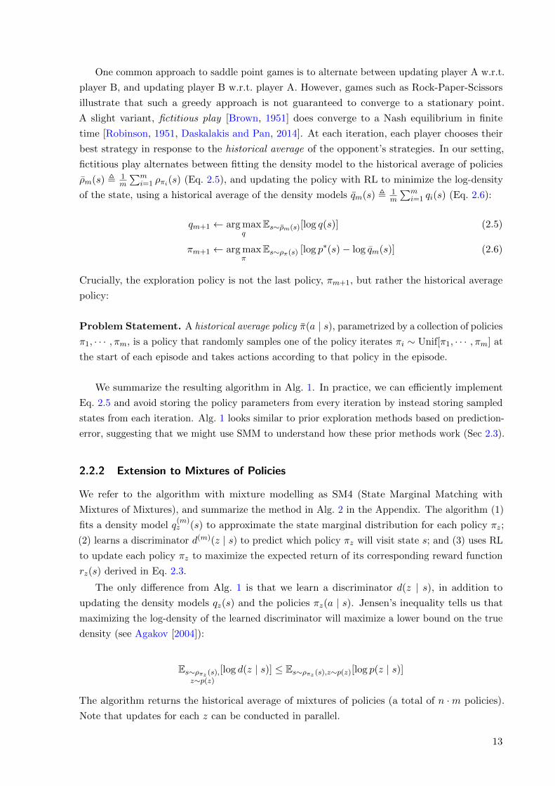
One common approach to saddle point games is to alternate between updating player A w.r.t.

player B, and updating player B w.r.t. player A. However, games such as Rock-Paper-Scissors

illustrate that such a greedy approach is not guaranteed to converge to a stationary point.

A slight variant, fictitious play [Brown, 1951] does converge to a Nash equilibrium in finite

time [Robinson, 1951, Daskalakis and Pan, 2014]. At each iteration, each player chooses their

best strategy in response to the historical average of the opponent’s strategies. In our setting,

fictitious play alternates between fitting the density model to the historical average of policies

ρm(s) , 1m

∑mi=1 ρπi(s) (Eq. 2.5), and updating the policy with RL to minimize the log-density

of the state, using a historical average of the density models qm(s) , 1m

∑mi=1 qi(s) (Eq. 2.6):

qm+1 ← arg maxq

Es∼ρm(s)[log q(s)] (2.5)

πm+1 ← arg maxπ

Es∼ρπ(s) [log p∗(s)− log qm(s)] (2.6)

Crucially, the exploration policy is not the last policy, πm+1, but rather the historical average

policy:

Problem Statement. A historical average policy π(a | s), parametrized by a collection of policies

π1, · · · , πm, is a policy that randomly samples one of the policy iterates πi ∼ Unif[π1, · · · , πm] at

the start of each episode and takes actions according to that policy in the episode.

We summarize the resulting algorithm in Alg. 1. In practice, we can efficiently implement

Eq. 2.5 and avoid storing the policy parameters from every iteration by instead storing sampled

states from each iteration. Alg. 1 looks similar to prior exploration methods based on prediction-

error, suggesting that we might use SMM to understand how these prior methods work (Sec 2.3).

2.2.2 Extension to Mixtures of Policies

We refer to the algorithm with mixture modelling as SM4 (State Marginal Matching with

Mixtures of Mixtures), and summarize the method in Alg. 2 in the Appendix. The algorithm (1)

fits a density model q(m)z (s) to approximate the state marginal distribution for each policy πz;

(2) learns a discriminator d(m)(z | s) to predict which policy πz will visit state s; and (3) uses RL

to update each policy πz to maximize the expected return of its corresponding reward function

rz(s) derived in Eq. 2.3.

The only difference from Alg. 1 is that we learn a discriminator d(z | s), in addition to

updating the density models qz(s) and the policies πz(a | s). Jensen’s inequality tells us that

maximizing the log-density of the learned discriminator will maximize a lower bound on the true

density (see Agakov [2004]):

Es∼ρπz (s),z∼p(z)

[log d(z | s)] ≤ Es∼ρπz (s),z∼p(z)[log p(z | s)]

The algorithm returns the historical average of mixtures of policies (a total of n ·m policies).

Note that updates for each z can be conducted in parallel.

13

inputs targets prior

SMM (Ours) s s 3

RND s e(s) 7

Forward Models s, a s′ 7

Inverse Models s, s′ a 7

Table 2.1: Exploration based on predictive-error: A number of exploration methods operateby learning a function that predicts some target quantity given some input quantities, and usingthis function’s error as an exploration bonus. Previous methods have omitted the prior term,which our method implicitly incorporates via historical averaging.

2.3 Prediction-Error Exploration is Approximate State Marginal

Matching

This section compares and contrasts SMM with prior exploration methods that use predictive-

error, showing that these methods approximately optimize the same SMM objective when

averaged over time, but otherwise exhibits oscillatory learning dynamics. Both the objectives

and the optimization procedures are similar, but contain important yet subtle differences.

Objectives As introduced in Proposition 2.2.1, the state marginal matching objective can be

viewed as a min-max objective (Eq. 2.4). When the density model is a VAE and the target

distribution p∗(s) is uniform, this min-max objective looks like the prediction error between a

state and itself, plus a regularizer:

maxπ

minψ

Eρπ(s)

[‖fψ(st)− st‖22

]+Rπ(ψ),

where fφ is our autoencoder and Rπ(ψ) is the KL penalty on the VAE encoder for the data

distribution ρπ(s). Prior exploration methods look quite similar. For example, Exploration

methods based on predictive error also optimize a min-max objective. For example, the objective

for RND [Burda et al., 2018] is

maxπ

minψ

Eρπ(s)

[‖fψ(st)− e(st)‖22

],

where e(·) is an encoder obtained by a randomly initialized neural network. Exploration bonuses

based on the predictive error of forward models [Schmidhuber, 1991, Chentanez et al., 2005,

Stadie et al., 2015] have a similar form, but instead consider full transitions:

maxπ

minψ

Eρπ(s)

[‖fψ(st, at)− st+1‖22

].

Exploration bonuses derived from inverse models [Pathak et al., 2017] look similar:

maxπ

minψ

Eρπ(s)

∥∥fψ(st, st+1)− at‖22].

We summarize these methods in Table 2.1. We believe that the prior term R(ψ) in the SMM

objective (Eq. 2.3) that is omitted from the other objectives possibly explains why SMM continues

to explore at convergence.

14

(a) State Marginals (b) Oscillatory Learning

Figure 2.2: Gridworld environment with a “noisy TV” state at the intersection of the twohallways (see Section 2.3.1). (Left) State Marginals of various exploration methods. (Right)Without historical averaging, two-player games exhibit oscillatory learning dynamics.

Optimization Both SMM and prior exploration methods employ alternating optimization to

solve their respective min-max problems. Prior work uses a greedy procedure that optimizes

the policy w.r.t. the current auxiliary model, and optimizes the auxiliary model w.r.t. the

current policy. This greedy procedure often fails to converge, as we demonstrate experimentally

in Section 2.3.1. In contrast, SMM uses fictitious play, a slight modification that optimizes the

policy w.r.t. the historical average of the auxiliary models and optimizes the auxiliary model w.r.t.

the historical average of the policies. Unlike the greedy approach, fictitious play is guaranteed to

converge. This difference may explain why SMM learns better exploratory policies than prior

methods.

While prior works use a procedure that is not guaranteed to converge, they nonetheless

excel at solving hard exploration tasks. We draw an analogy to fictitious play to explain their

success. While these methods never acquire an exploratory policy, over the course of training

they will eventually visit all states. In other words, the historical average over policies will visit

a wide range of states. Since the replay buffer exactly corresponds to this historical average over

states, these methods will obtain a replay buffer with a diverse range of experience, possibly

explaining why they succeed at solving hard exploration tasks. Moreover, this analysis suggests a

surprisingly simple method for obtaining an exploration from these prior methods: use a mixture

of the policy iterates throughout training. The following section will not only compare SMM

against prior exploration methods, but also show that this historical averaging trick can be used

to improve existing exploration methods.

15

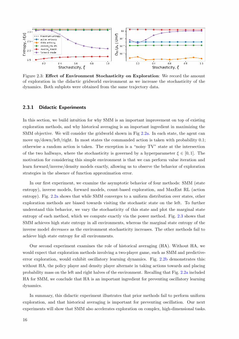
Figure 2.3: Effect of Environment Stochasticity on Exploration: We record the amountof exploration in the didactic gridworld environment as we increase the stochasticity of thedynamics. Both subplots were obtained from the same trajectory data.

2.3.1 Didactic Experiments

In this section, we build intuition for why SMM is an important improvement on top of existing

exploration methods, and why historical averaging is an important ingredient in maximizing the

SMM objective. We will consider the gridworld shown in Fig 2.2a. In each state, the agent can

move up/down/left/right. In most states the commanded action is taken with probability 0.1;

otherwise a random action is taken. The exception is a “noisy TV” state at the intersection

of the two hallways, where the stochasticity is governed by a hyperparameter ξ ∈ [0, 1]. The

motivation for considering this simple environment is that we can perform value iteration and

learn forward/inverse/density models exactly, allowing us to observe the behavior of exploration

strategies in the absence of function approximation error.

In our first experiment, we examine the asymptotic behavior of four methods: SMM (state

entropy), inverse models, forward models, count-based exploration, and MaxEnt RL (action

entropy). Fig. 2.2a shows that while SMM converges to a uniform distribution over states, other

exploration methods are biased towards visiting the stochastic state on the left. To further

understand this behavior, we vary the stochasticity of this state and plot the marginal state

entropy of each method, which we compute exactly via the power method. Fig. 2.3 shows that

SMM achieves high state entropy in all environments, whereas the marginal state entropy of the

inverse model decreases as the environment stochasticity increases. The other methods fail to

achieve high state entropy for all environments.

Our second experiment examines the role of historical averaging (HA). Without HA, we

would expect that exploration methods involving a two-player game, such as SMM and predictive-

error exploration, would exhibit oscillatory learning dynamics. Fig. 2.2b demonstrates this:

without HA, the policy player and density player alternate in taking actions towards and placing

probability mass on the left and right halves of the environment. Recalling that Fig. 2.2a included

HA for SMM, we conclude that HA is an important ingredient for preventing oscillatory learning

dynamics.

In summary, this didactic experiment illustrates that prior methods fail to perform uniform

exploration, and that historical averaging is important for preventing oscillation. Our next

experiments will show that SMM also accelerates exploration on complex, high-dimensional tasks.

16

(a) Fetch environment (b) D’Claw robot

Hall Length

Initial StateGoal

(c) Navigation env.

Figure 2.4: Environments: We ran experiments in both a simulated and real-world manipula-tion environments (a-b), as well as a pointmass navigation environment (c). In the Navigationenvironment, a point-mass agent is spawned at the center of m long hallways that extend radiallyoutward, and the target state distribution places uniform probability mass 1

m at the end of eachhallway. We can vary the length of the hallway and the number of hallways to control the taskdifficulty.

2.4 Experimental Evaluation

In this section, we empirically study whether our method learns to explore effectively when

scaled to more complex RL benchmarks, and compare against prior exploration methods.

Our experiments demonstrate how State Marginal Matching provides good exploration, a key

component of which is the historical averaging step.

We compare to a state-of-the-art off-policy MaxEnt RL algorithm, Soft Actor-Critic (SAC) [Haarnoja

et al., 2018]; an inverse RL algorithm, Generative Adversarial Imitation Learning (GAIL) [Ho

and Ermon, 2016]; and three exploration methods:

• Count-based Exploration (Count), which discretizes states and uses − log π(s) as an

exploration bonus.

• Pseudo-counts (PC) [Bellemare et al., 2016], which uses the recoding probability as a bonus.

• Intrinsic Curiosity Module (ICM) [Pathak et al., 2017], which uses prediction error as a

bonus.

All exploration methods have access to exactly the same information and the same extrinsic

reward function. SMM interprets this extrinsic reward as the log probability of a target

distribution: p∗(s) ∝ exp(renv(s)).

We used SAC as the base RL algorithm for all exploration methods (SMM, Count, PC, ICM).

For all algorithms, we use a Gaussian policy with two hidden layers with Tanh activation and a

final fully-connected layer. The Value function and Q-function each are a feedforward MLP with

two hidden layers with ReLU activation and a final fully-connected layer. Each hidden layer is

of size 300 (SMM, SAC, ICM, C, PC) or 256 (GAIL). The same network configuration is used

for the SMM discriminator, d(z | s), and the GAIL discriminator, but with different input and

output sizes.

17

We use a variational autoencoder (VAE) to model the density q(s) for both SMM and

Pseudocounts. The VAE encoder and decoder networks each consist of two hidden layers of size

(150, 150) with ReLU activation.

In our SMM implementation, we estimated the density of data x as p(x) ≈ decoder(x = x|z =

encoder(x)). That is, we encoded x to z, reconstruction x from z, and then took the likelihood

of the true data x under a unit-variance Gaussian distribution centered at the reconstructed

x. The log-likelihood is therefore given by the mean-squared error between the data x and the

reconstruction x, plus a constant that is independent of x: log q(x) = 12‖x− x‖

22 + C.

For SMM, we approximate the historical average of density models (Eq. 2.6) with the most

recent iterate, and use a uniform categorical distribution for the prior p(z). To train GAIL, we

generated synthetic expert data by sampling expert states from the target distribution p∗(s).

Results for all experiments are averaged over 4-5 random seeds. Additional details about the

experimental setup can be found in Appendix A.1.

2.4.1 Environments

We ran experiments in various manipulation and navigation environments, shown in Fig 2.4. We

summarize the environments and the target state marginal distributions below.

Fetch. We used a simulated Fetch environment [Plappert et al., 2018] consisting of a single

gripper arm and a block object on top of the table (Fig. 2.4a). The state vector s ∈ R28 includes

the xyz-coordinates sobj, srobot ∈ R3 of the block and the robot gripper respectively, as well as

their velocities, orientations, and relative position sobj − srobot. At the beginning of each episode,

we spawn the object at the center of the table, and the robot gripper above the initial block

position. We terminate each episode after 50 environment steps, or if the block falls off the table.

We considered two target state marginal distributions. In Fetch-Uniform, we defined the

target distribution to be uniform over the entire state space (joint + block configuration), with

the constraints that we put low probability mass on states where the block has fallen off the

table; that actions should be small; and that the arm should be close to the object. The target

density is given by

p∗(s) ∝ exp (α1rgoal(s) + α2rrobot(s) + α3raction(s))

where α1, α2, α3 > 0 are fixed weights, and the rewards

rgoal(s) := 1− 1(sobj is on the table surface)

rrobot(s) := 1(‖sobj − srobot‖22 < 0.1)

raction(s) := −‖a‖22

correspond to (1) a uniform distribution of the block position over the table surface (the agent

receives +0 reward while the block is on the table), (2) an indicator reward for moving the

robot gripper close to the block, and (3) action penalty, respectively. The environment reward

is a weighted sum of the three reward terms: renv(s) , 20rgoal(s) + rrobot(s) + 0.1raction(s). At

test-time, we sample a goal block location g ∈ R3 uniformly on the table surface, and the goal is

not observed by the agent.

18

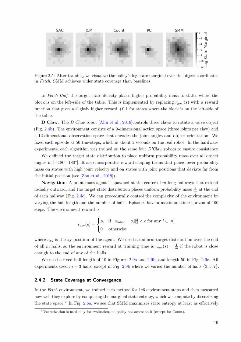
Figure 2.5: After training, we visualize the policy’s log state marginal over the object coordinatesin Fetch. SMM achieves wider state coverage than baselines.

In Fetch-Half, the target state density places higher probability mass to states where the

block is on the left-side of the table. This is implemented by replacing rgoal(s) with a reward

function that gives a slightly higher reward +0.1 for states where the block is on the left-side of

the table.

D’Claw. The D’Claw robot [Ahn et al., 2019]controls three claws to rotate a valve object

(Fig. 2.4b). The environment consists of a 9-dimensional action space (three joints per claw) and

a 12-dimensional observation space that encodes the joint angles and object orientation. We

fixed each episode at 50 timesteps, which is about 5 seconds on the real robot. In the hardware

experiments, each algorithm was trained on the same four D’Claw robots to ensure consistency.

We defined the target state distribution to place uniform probability mass over all object

angles in [−180◦, 180◦]. It also incorporates reward shaping terms that place lower probability

mass on states with high joint velocity and on states with joint positions that deviate far from

the initial position (see [Zhu et al., 2019]).

Navigation: A point-mass agent is spawned at the center of m long hallways that extend

radially outward, and the target state distribution places uniform probability mass 1m at the end

of each hallway (Fig. 2.4c). We can procedurally control the complexity of the environment by

varying the hall length and the number of halls. Episodes have a maximum time horizon of 100

steps. The environment reward is

renv(s) =

pi if ‖srobot − gi‖22 < ε for any i ∈ [n]

0 otherwise

where sxy is the xy-position of the agent. We used a uniform target distribution over the end

of all m halls, so the environment reward at training time is renv(s) = 1m if the robot is close

enough to the end of any of the halls.

We used a fixed hall length of 10 in Figures 2.9a and 2.9b, and length 50 in Fig. 2.9c. All

experiments used m = 3 halls, except in Fig. 2.9b where we varied the number of halls {3, 5, 7}.

2.4.2 State Coverage at Convergence

In the Fetch environment, we trained each method for 1e6 environment steps and then measured

how well they explore by computing the marginal state entropy, which we compute by discretizing

the state space.2 In Fig. 2.6a, we see that SMM maximizes state entropy at least as effectively

2Discretization is used only for evaluation, no policy has access to it (except for Count).

19

(a) Fetch environment (b) Sim2Real on D’Claw

Figure 2.6: The Exploration of SMM: (a) In the Fetch environment, we plot the policy’sstate entropy over the object and gripper coordinates, averaged over 1,000 epochs. SMM exploresmore than baselines, as indicated by the larger state entropy (larger is better). (b) In theD’Claw environment, we trained policies in simulation and then observed how far the trainedpolicy rotated the knob on the hardware robot, measuring both the total number of rotationsand the minimum and maximum valve rotations. SMM turns the knob further to the left andright than the baselines, and also completes a larger cumulative number of rotations.

Figure 2.7: Training on Hardware (D’Claw): We trained SAC and SMM on the real robotfor 1e5 environment steps (about 9 hours in real time), and measured the angle turned throughouttraining. We see that SMM moves the knob more and visits a wider range of states than SAC.All results are averaged over 4-5 seeds.

as prior methods, if not better. While this comparison is somewhat unfair, as we measure

exploration using the objective that SMM maximizes, none of the methods we compare against

propose an alternative metric for exploration.

On the D’Claw robot, we trained SMM and other baselines in simulation, and then evaluated

the acquired exploration policy on the real robot using two metrics: the total number of rotations

(in either direction), and the maximum radians turned (in both directions). For each method,

we computed the average metric across 100 evaluation episodes. We repeated this process for 5

independent training runs. Compared to the baselines, SMM turns the knob more to a wider

range of angles (Fig. 2.6b). To test for statistical significance, we used a 1-sided Student’s t-test

to test the hypothesis that SMM turned the knob more to a wider range of angles than SAC.

The p-values were all less than 0.05: p = 0.046 for number of rotations, p = 0.019 for maximum

clockwise angle, and p = 0.001 for maximum counter-clockwise angle. The results on the D’Claw

hardware robot suggests that exploration techniques may actually be useful in the real world,

which may encourage future work to study exploration methods on real-world tasks.

We also investigated whether it was possible to learn an exploration policy directly in the

real world, without the need for a simulator, an important setting in scenarios where faithful

simulators are hard to build. In Fig. 2.7, we plot the range of angles that the policy explores

20

(a) Test-time adaptation (b) SMM ablation

Figure 2.8: Fast Adaptation: (a) We plot the percentage of test-time goals found withinN episodes. SMM and its mixture-model variant SM4 both explore faster than the baselines,allowing it to successfully find the goal in fewer episodes. (b) We compare SMM/SM4 withdifferent numbers of mixtures, and with vs. without historical averaging. Increasing the numberof latent mixture components n ∈ {1, 2, 4} accelerates exploration, as does historical averaging.Error bars show std. dev. across 4 random seeds.

throughout training. Not only does SMM explore a wider range of angles than SAC, but its

ability to explore increases throughout training, suggesting that the SMM objective is correlated

with real-world metrics of exploration.

2.4.3 Test-time Exploration

We also evaluated whether the exploration policy acquired by SMM allows us to solve downstream

tasks more quickly. As shown in Fig. 2.8a, SMM and its mixture variant, SM4, both adapt

substantially more quickly than other exploration methods, achieving a success rate 20% higher

than the next best method, and reaching the same level of performance of the next baseline

(ICM) in 4x fewer episodes.

Ablation Study. In Fig. 2.8b, we study the effect of mixture modelling on test-time

exploration. After running SMM/SM4 with a uniform distribution, we count the number of

episodes required to find an (unknown) goal state. We run each method for the same number

of environment transitions; a mixture of three policies does not get to take three times more

transitions. We find that increasing the number of mixture components increases the agents

success. However, the effect was smaller when using historical averaging. Taken together, this

result suggests that efficient exploration requires either historical averaging or mixture modelling,

but might not need both. In particular, SMM without historical averaging attains similar

performance as the next best baseline (ICM), suggesting that historical averaging is the key

ingredient, while the particular choice of prediction error or VAE is less important.

2.4.4 Exploration in State Space vs. Action Space

Is exploration in state space (as done by SMM) better than exploration in action space (as done

by MaxEnt RL, e.g., SAC)? To study this question, we implemented a Navigation environment,

shown in Fig. 2.4c. To evaluate each method, we counted the number of hallways that the agent

21

SAC SMM

3 Halls of length 10

(a) ρπ(s) (b) % Goals reached during training

0 20 40 60 80 100Epoch

0

10

20

30

40

50

60

Retu

rn

Length 50 HallwayOursw/o H[s|z]w/o H[z|s]SAC

(c) Train-time Performance

Figure 2.9: Exploration in State Space (SMM) vs. Action Space (SAC) for Navi-gation : (a) A heatmap showing states visited by SAC and SMM during training illustratesthat SMM explores a wider range of states. (b) SMM reaches more goals than the MaxEntbaseline. SM4 is an extension of SMM that incorporates mixture modelling with n > 1 skills (seeAppendix 2.1.3), and further improves exploration of SMM. (c) Ablation Analysis of SM4.On the Navigation task, we compare SM4 (with three mixture components) against ablationbaselines that lack conditional state entropy, latent conditional action entropy, or both (i.e., SAC)in the SM4 objective (Eq. 2.3). We see that both terms contribute heavily to the explorationability of SM4, but the state entropy term is especially critical.

Figure 2.10: With vs. Without Historical Averaging: After training, we rollout the policyfor 1e3 epochs, and record the entropy of the object and gripper positions in Fetch. SMMachieves higher state entropy than the other methods. Historical averaging also helps previousexploration methods achieve greater state coverage.

fully explored (i.e., reached the end) during training. Fig. 2.9a shows the state visitations for

the three hallway environment, illustrating that SAC only explores one hallway, whereas SMM

explores all three. Fig. 2.9b also shows that SMM consistently explores 60% of hallways, whereas

SAC rarely visits more than 20% of hallways.

2.4.5 Does Historical Averaging help other baselines?

In Fig. 2.10, we see that historical averaging is not only beneficial to SMM, but also improves the

exploration of prior methods. The result further supports our hypothesis that prior exploration

methods are approximately optimizing the same SMM objective.

2.4.6 Non-Uniform Exploration

We check whether prior knowledge injected via the target distribution is reflected in the policy

obtained from State Marginal Matching. Using the same Fetch environment as above, we modified

the target distribution to assign larger probability to states where the block was on the left half

22

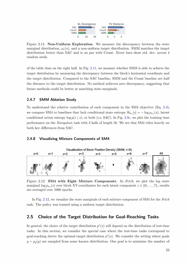
0 20 40

SACCountSMM

KL Divergence

0 2 4

SACCountSMM

TV Distance

Figure 2.11: Non-Uniform Exploration: We measure the discrepancy between the statemarginal distribution, ρπ(s), and a non-uniform target distribution. SMM matches the targetdistribution better than SAC and is on par with Count. Error bars show std. dev. across 4random seeds.

of the table than on the right half. In Fig. 2.11, we measure whether SMM is able to achieve the

target distribution by measuring the discrepancy between the block’s horizontal coordinate and

the target distribution. Compared to the SAC baseline, SMM and the Count baseline are half

the distance to the target distribution. No method achieves zero discrepancy, suggesting that

future methods could be better at matching state marginals.

2.4.7 SMM Ablation Study

To understand the relative contribution of each component in the SM4 objective (Eq. 2.3),

we compare SM4 to baselines that lack conditional state entropy Hπz [s] = − log ρπz(s), latent

conditional action entropy log p(z | s), or both (i.e, SAC). In Fig. 2.9c, we plot the training time

performance on the Navigation task with 3 halls of length 50. We see that SM4 relies heavily on

both key differences from SAC.

2.4.8 Visualizing Mixture Components of SM4

Figure 2.12: SM4 with Eight Mixture Components. In Fetch, we plot the log statemarginal log ρπz(s) over block XY-coordinates for each latent component z ∈ {0, . . . , 7}, resultsare averaged over 1000 epochs.

In Fig. 2.12, we visualize the state marginals of each mixture component of SM4 for the Fetch

task. The policy was trained using a uniform target distribution.

2.5 Choice of the Target Distribution for Goal-Reaching Tasks

In general, the choice of the target distribution p∗(s) will depend on the distribution of test-time

tasks. In this section, we consider the special case where the test-time tasks correspond to

goal-reaching derive the optimal target distribution p∗(s). We consider the setting where goals

g ∼ pg(g) are sampled from some known distribution. Our goal is to minimize the number of

23

episodes required to reach that goal state. We define reaching the goal state as visiting a state

that lies within an ε ball of the goal, where both ε > 0 and the distance metric are known.

We start with a simple lemma that shows that the probability that we reach the goal at any

state in a trajectory is at least the probability that we reach the goal at a randomly chosen state

in that same trajectory. Defining the binary random variable zt , 1(‖st − g‖ ≤ ε) as the event

that the state at time t reaches the goal state, we can formally state the claim as follows:

Lemma 2.5.1.

p

(T∑t=1

zt > 0

)≥ p(zt) where t ∼ Unif [1, · · · , H]

Proof. We start by noting the following implication:

zt = 1 =⇒T∑t=1

zt > 0

Thus, the probability of the event on the RHS must be at least as large as the probability of the

event on the LHS:

p(zt) ≤ p

(T∑t=1

zt > 0

)

Next, we look at the expected number of episodes to reach the goal state. Since each episode

is independent, the expected hitting time is simply

HittingTime(s) =1

p(some state reaches s)

=1

p(∑T

t=1 zt > 0) ≤ 1

p(zt)

Note that we have upper-bounded the hitting time using Lemma 2.5.1. Since the goal g is a

random variable, we take an expectation over g:

Es∼pg(s) [HittingTime(s)] ≤ Es∼pg(s)

[1

p(zt)

]≤ Es∼pg(s)

[1∫

p∗(s)1(‖s− s‖ ≤ ε)ds

], F(p∗)

where p∗(s) denotes the target state marginal distribution. We will minimize F , an upper bound

on the expected hitting time.

Lemma 2.5.2. The state marginal distribution p∗(s) ∝√p(s) minimizes F(p∗), where

p(s) ,∫pg(s)1(‖s− s‖ ≤ ε)ds

is a smoothed version of the target density.

24

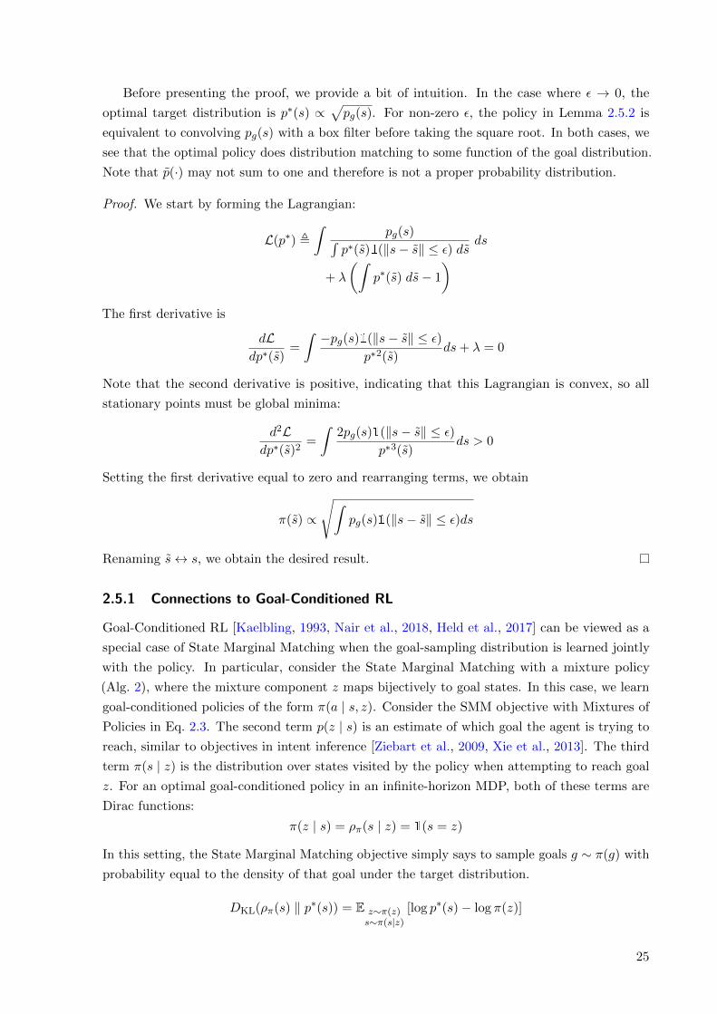
Before presenting the proof, we provide a bit of intuition. In the case where ε → 0, the

optimal target distribution is p∗(s) ∝√pg(s). For non-zero ε, the policy in Lemma 2.5.2 is

equivalent to convolving pg(s) with a box filter before taking the square root. In both cases, we

see that the optimal policy does distribution matching to some function of the goal distribution.

Note that p(·) may not sum to one and therefore is not a proper probability distribution.

Proof. We start by forming the Lagrangian:

L(p∗) ,∫

pg(s)∫p∗(s)1(‖s− s‖ ≤ ε) ds

ds

+ λ

(∫p∗(s) ds− 1

)The first derivative is

dLdp∗(s)

=

∫ −pg(s)1(‖s− s‖ ≤ ε)p∗2(s)

ds+ λ = 0

Note that the second derivative is positive, indicating that this Lagrangian is convex, so all

stationary points must be global minima:

d2Ldp∗(s)2

=

∫2pg(s)1(‖s− s‖ ≤ ε)

p∗3(s)ds > 0

Setting the first derivative equal to zero and rearranging terms, we obtain

π(s) ∝

√∫pg(s)1(‖s− s‖ ≤ ε)ds

Renaming s↔ s, we obtain the desired result.

2.5.1 Connections to Goal-Conditioned RL

Goal-Conditioned RL [Kaelbling, 1993, Nair et al., 2018, Held et al., 2017] can be viewed as a

special case of State Marginal Matching when the goal-sampling distribution is learned jointly

with the policy. In particular, consider the State Marginal Matching with a mixture policy

(Alg. 2), where the mixture component z maps bijectively to goal states. In this case, we learn

goal-conditioned policies of the form π(a | s, z). Consider the SMM objective with Mixtures of

Policies in Eq. 2.3. The second term p(z | s) is an estimate of which goal the agent is trying to

reach, similar to objectives in intent inference [Ziebart et al., 2009, Xie et al., 2013]. The third

term π(s | z) is the distribution over states visited by the policy when attempting to reach goal

z. For an optimal goal-conditioned policy in an infinite-horizon MDP, both of these terms are

Dirac functions:

π(z | s) = ρπ(s | z) = 1(s = z)

In this setting, the State Marginal Matching objective simply says to sample goals g ∼ π(g) with

probability equal to the density of that goal under the target distribution.

DKL(ρπ(s) ‖ p∗(s)) = E z∼π(z)s∼π(s|z)

[log p∗(s)− log π(z)]

25

Whether goal-conditioned RL is the preferable way to do distribution matching depends on

(1) the difficulty of sampling goals and (2) the supervision that will be provided at test time. It

is natural to use goal-conditioned RL in settings where it is easy to sample goals, such as when

the space of goals is small and finite or otherwise low-dimensional. If a large collection of goals is

available apriori, we could use importance sampling to generate goals to train the goal-conditioned

policy [Pong et al., 2019]. However, many real-world settings have high-dimensional goals, which

can be challenging to sample. While goal-conditioned RL is likely the right approach when we

will be given a test-time task, a latent-conditioned policy may explore better in settings where

the goal-state is not provided at test-time.

2.6 Related Work

Many exploration algorithms can be classified by whether they explore in the space of actions,

policy parameters, goals, or states. Common exploration strategies including ε-greedy and

Ornstein–Uhlenbeck noise [Lillicrap et al., 2015], and MaxEnt RL algorithms [Ziebart, 2010,

Haarnoja et al., 2018] explore in the action space. Fortunato et al. [2017], Plappert et al. [2017]

show that adding parameter noise to the policy can result in good exploration.

Most closely related to our work are methods that perform exploration in the space of states or

goals [Colas et al., 2018, Held et al., 2017, Nair et al., 2018, Pong et al., 2019, Hazan et al., 2018].

While the state marginal matching objective is also considered in Hazan et al. [2018], our work

builds upon this prior work in a number of dimensions. First, we explain how to do distribution

matching properly by analyzing the SMM objective as a two-player game and applying historical

averaging from fictitious play. Our analysis also leads to a unified view of a large class of

existing intrinsic motivation techniques that previously were proposed as exploration heuristics,

showing that in fact these methods almost perform state marginal matching. Furthermore, we

introduce the notion that this objective yields a task-agnostic “policy prior” that can quickly

solve new tasks, and demonstrate this empirically on complex RL benchmarks. We also prove

that the SMM objective induces the optimal exploration for a certain class of goal-reaching tasks

(Appendix 2.5).

One class of exploration methods uses prediction error of some auxiliary task as an exploration

bonus, which provides high (intrinsic) reward in states where the predictive model performs

poorly [Pathak et al., 2017, Oudeyer et al., 2007, Schmidhuber, 1991, Houthooft et al., 2016, Burda

et al., 2018]. Another set of approaches [Tang et al., 2017, Bellemare et al., 2016, Schmidhuber,

2010] directly encourage the agent to visit novel states. While all methods effectively explore

during the course of solving a single task [Taıga et al., 2019], we showed in Sec. 2.3 that the

policy obtained at convergence is often not a good exploration policy by itself. In contrast, our

method converges to a highly-exploratory policy by maximizing state entropy.

The problems of exploration and meta-RL are tightly coupled. Meta-RL algorithms [Duan

et al., 2016, Finn et al., 2017, Rakelly et al., 2019, Mishra et al., 2017] must perform effective

exploration if they hope to solve a downstream task. Some prior work has explicitly looked at

the problem of learning to explore [Gupta et al., 2018, Xu et al., 2018]. Our problem statement is

similar to meta-learning, in that we also aim to learn a policy as a prior for solving downstream

tasks. However, whereas meta-RL requires a distribution of task reward functions, our method

26

requires only a single target state marginal distribution. Due to the simpler problem assumptions

and training procedure, our method may be easier to apply in real-world domains.

Related to our approach are maximum action entropy algorithms [Haarnoja et al., 2018,

Kappen et al., 2012, Rawlik et al., 2013, Ziebart et al., 2008, Theodorou and Todorov, 2012].

While these algorithms are referred to as MaxEnt RL, they are maximizing entropy over actions,

not states. These algorithms can be viewed as performing inference on a graphical model where

the likelihood of a trajectory is given by its exponentiated reward [Toussaint and Storkey, 2006,

Levine, 2018, Abdolmaleki et al., 2018]. While distributions over trajectories induce distributions

over states, computing the exact relationship requires integrating over all possible trajectories, an

intractable problem for most MDPs. A related but distinct class of relative entropy methods use

a similar entropy-based objective to limit the size of policy updates [Peters et al., 2010, Schulman

et al., 2015].

Many of the underlying ingredients of our method, such as adversarial games and density

estimation, have seen recent progress in imitation learning [Ziebart et al., 2008, Ho and Ermon,

2016, Finn et al., 2016a, Fu et al., 2017]. Similar to some inverse RL algorithms [Ho and Ermon,

2016, Fu et al., 2018a], our method iterates between learning a policy and learning a reward

function, though our reward function is obtained via a density model instead of a discriminator.

While inverse RL algorithms assume access to expert trajectories, we instead assume access to

the density of the target state marginal distribution. In many realistic settings, such as robotic

control with many degrees of freedom, providing fully-specified trajectories may be much more

challenging than defining a target state marginal distribution. The latter only requires some

aggregate statistics about expert behavior, and does not even need to be realizable by any policy.

2.7 Discussion

This work studied state marginal matching as a formal objective for exploration. While it is

often unclear what existing exploration methods will converge to, the SMM objective has a clear

solution: at convergence, the policy should visit states in proportion to their density under a

target distribution. The resulting policy can be used as a prior in a multi-task setting to amortize

exploration and adapt more quickly to new, potentially sparse, reward functions.

We explain how to perform distribution matching properly via historical averaging. We

further demonstrate that prior work approximately maximizes the SMM objective, offering an

explanation for the success of these methods. Augmenting these prior methods with an important

historical averaging step not only guarantees that they converge, but also empirically improves

their exploration. Experiments on both simulated and real-world tasks demonstrated how SMM

learns to explore, enabling an agent to efficiently explore in new tasks provided at test time.

In summary, our work unifies prior exploration methods as performing approximate distribu-

tion matching, and explains how state distribution matching can be performed properly. This

perspective provides a clearer picture of exploration, and is useful particularly because many of

the underlying ingredients, such as adversarial games and density estimation, have seen recent

progress and therefore might be adopted to improve exploration methods.

One limitation of many exploration algorithms, including state marginal matching, is the

requirement of knowing a relatively low-dimensional state representation that informs the agent

27

along which state dimensions it should explore. However, learning a good state representation

requires data collected from a policy that does efficient exploration. This Catch-22 situation

between exploration and representation learning remains an unsolved challenge in RL. In

Chapter 3, we will look at how weakly-supervised representation learning can allow us to

scalably learn a structured representation for better exploration and learning.

28

Chapter 3

Weakly-Supervised RL for

Controllable Behavior

A general purpose agent must be able to efficiently learn a diverse array of tasks through

interacting with the real world. The typical approach is to manually define a set of reward

functions and only learn the tasks induced by these reward functions [Finn et al., 2017, Hausman

et al., 2018]. However, defining and tuning the reward functions is labor intensive and places

a significant burden on the user to specify reward functions for all tasks that they care about.

Designing reward functions that provide enough learning signal yet still induce the correct

behavior at convergence is challenging [Hadfield-Menell et al., 2017]. An alternative approach is

to parametrize a family of tasks, such as goal-reaching tasks, and learn a policy for each task in

this family [Hazan et al., 2018, Pong et al., 2019, Lee et al., 2019b, Ghasemipour et al., 2019,

Stanley and Miikkulainen, 2002, Pugh et al., 2016]. However, learning a single goal-conditioned

policy for reaching all goals is a challenging optimization problem and is prone to underfitting,

especially in high-dimensional tasks with limited data [Dasari et al., 2019]. In this work, we aim

to accelerate the acquisition of goal-conditioned policies by narrowing the goal space through

weak supervision. Answering this question would allow an RL agent to prioritize exploring and

learning meaningful tasks, resulting in faster acquisition of behaviors for solving human-specified

tasks.

How might we constrain the space of tasks to those that are semantically meaningful? Reward

functions and demonstrations are the predominant approaches to training RL agents, but they

are expensive to acquire [Hadfield-Menell et al., 2017]. Generally, demonstrations require expert

humans to be present [Finn et al., 2016a, Duan et al., 2017, Laskey et al., 2017], and it remains

a challenge to acquire high-quality demonstration data from crowdsourcing [Mandlekar et al.,

2018]. In contrast, human preferences and ranking schemes provide an interface for sources of

supervision that are easy and intuitive for humans to specify [Christiano et al., 2017], and can

scale with the collection of offline data via crowd-sourcing. However, if we are interested in

learning many tasks rather than just one, these approaches do not effectively facilitate scalable

learning of many different tasks or goals.

In this work, we demonstrate how weak supervision provides useful information to agents with

minimal burden, and how agents can leverage that supervision when learning in an environment.

We will study one approach to using weak supervision in the goal-conditioned RL setting [Kael-

29

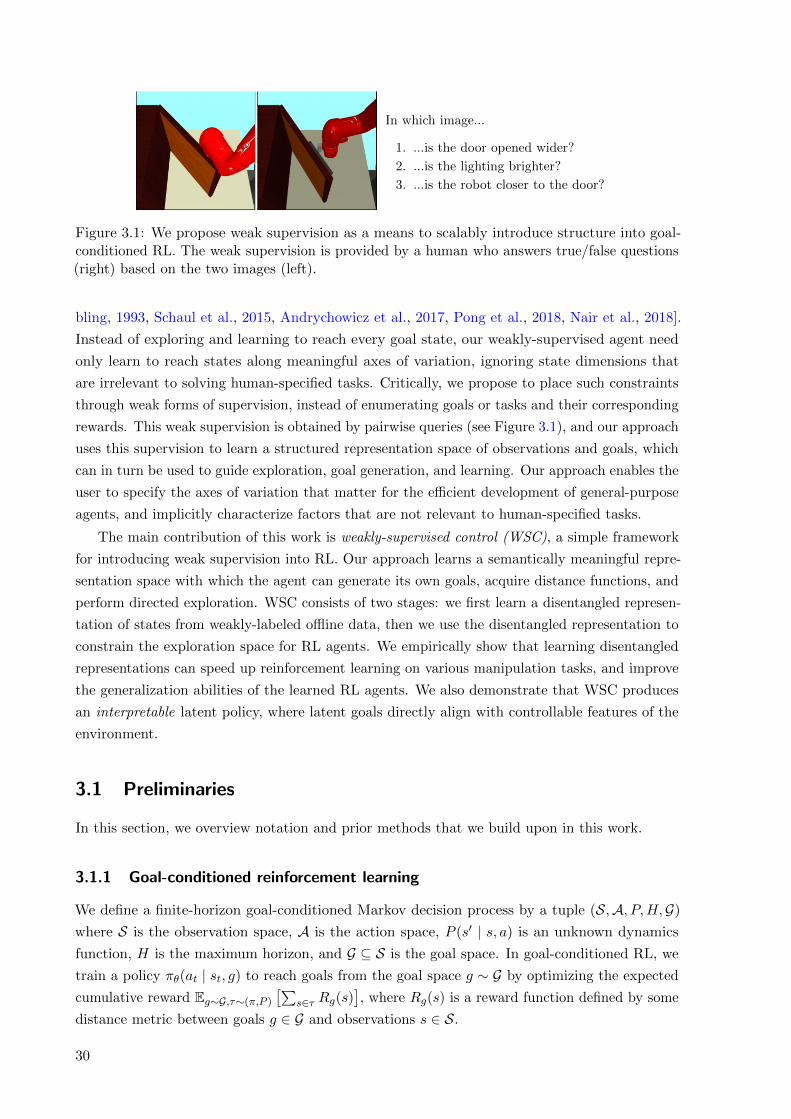
In which image...

1. ...is the door opened wider?

2. ...is the lighting brighter?

3. ...is the robot closer to the door?

Figure 3.1: We propose weak supervision as a means to scalably introduce structure into goal-conditioned RL. The weak supervision is provided by a human who answers true/false questions(right) based on the two images (left).

bling, 1993, Schaul et al., 2015, Andrychowicz et al., 2017, Pong et al., 2018, Nair et al., 2018].

Instead of exploring and learning to reach every goal state, our weakly-supervised agent need

only learn to reach states along meaningful axes of variation, ignoring state dimensions that

are irrelevant to solving human-specified tasks. Critically, we propose to place such constraints

through weak forms of supervision, instead of enumerating goals or tasks and their corresponding

rewards. This weak supervision is obtained by pairwise queries (see Figure 3.1), and our approach

uses this supervision to learn a structured representation space of observations and goals, which

can in turn be used to guide exploration, goal generation, and learning. Our approach enables the

user to specify the axes of variation that matter for the efficient development of general-purpose

agents, and implicitly characterize factors that are not relevant to human-specified tasks.

The main contribution of this work is weakly-supervised control (WSC), a simple framework

for introducing weak supervision into RL. Our approach learns a semantically meaningful repre-

sentation space with which the agent can generate its own goals, acquire distance functions, and

perform directed exploration. WSC consists of two stages: we first learn a disentangled represen-

tation of states from weakly-labeled offline data, then we use the disentangled representation to

constrain the exploration space for RL agents. We empirically show that learning disentangled

representations can speed up reinforcement learning on various manipulation tasks, and improve

the generalization abilities of the learned RL agents. We also demonstrate that WSC produces

an interpretable latent policy, where latent goals directly align with controllable features of the

environment.

3.1 Preliminaries

In this section, we overview notation and prior methods that we build upon in this work.

3.1.1 Goal-conditioned reinforcement learning

We define a finite-horizon goal-conditioned Markov decision process by a tuple (S,A, P,H,G)

where S is the observation space, A is the action space, P (s′ | s, a) is an unknown dynamics

function, H is the maximum horizon, and G ⊆ S is the goal space. In goal-conditioned RL, we

train a policy πθ(at | st, g) to reach goals from the goal space g ∼ G by optimizing the expected

cumulative reward Eg∼G,τ∼(π,P )

[∑s∈τ Rg(s)

], where Rg(s) is a reward function defined by some

distance metric between goals g ∈ G and observations s ∈ S.

30

Figure 3.2: Our method uses weak supervision, like that depicted in this figure, to directexploration and accelerate learning on visual manipulation tasks of varying complexity. Eachdata sample consists of a pair of image observations {s1, s2} and a factor label vector y ∈ {0, 1}K ,where yk = 1(fk(s1) < fk(s2)) indicates whether the kth factor of image s1 has smaller valuethan that of image s2. Example factors of variation include the gripper position, object positions,brightness, and door angle. Note that we only need to collect labels for the axes of variationthat may be relevant for future downstream tasks (see Appendix 3.4.5). In environments with‘light’ as a factor (e.g., PushLights), the lighting conditions change randomly at the start of eachepisode. In environments with ‘color’ as a factor (e.g., PickupColors), both the object colorand table color randomly change at the start of each episode. Bolded factors correspond to theuser-specified factor indices I indicating which of the factors are relevant for solving the class oftasks (see Sec. 3.2)

In low-dimensional tasks, one can simply take the reward to be the negative `2-distance in the

state space [Andrychowicz et al., 2017]. However, defining distance metrics is more challenging in

high-dimensional spaces, such as images [Yu et al., 2019]. Prior work on visual goal-conditioned

RL [Nair et al., 2018, Pong et al., 2019] train an additional state representation model, such as a

VAE encoder eVAE : S → ZVAE. Their methods train a policy over encoded states and goals,

and define rewards using `2-distance in latent space:

Rg(s) = −‖eVAE(s)− eVAE(g)‖22.

3.1.2 Weakly-supervised disentangled representations

Our approach leverages weakly-supervised disentangled representation learning in the context

of reinforcement learning. Disentangled representation learning aims to learn interpretable

representations of data, where each dimension of the representation measures a distinct factor of

variation, conditioned on which the data was generated (see Fig. 3.2 for examples of factors).

More formally, consider data-generating processes where (f1, . . . , fK) ∈ F are the factors of

variation, and observations s ∈ S are generated from a function g∗ : F → S. We would like to

learn a disentangled latent representation e : S → Z such that, for any factor subindices I ⊆ [K],

the subset of latent values eI(s) = zI are only influenced by the true factors fI , and conversely,

e\I(s) = z\I are only influenced by f\I .

We consider a form of weak supervision called rank pairing, where data samples D :=

{(s1, s2, y)} consist of pairs of observations {s1, s2} and weak binary labels y ∈ {0, 1}K , where

31

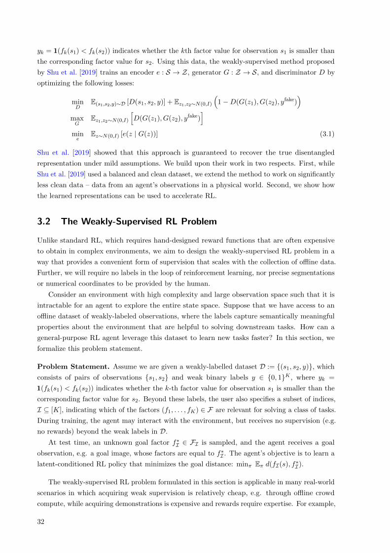
yk = 1(fk(s1) < fk(s2)) indicates whether the kth factor value for observation s1 is smaller than

the corresponding factor value for s2. Using this data, the weakly-supervised method proposed

by Shu et al. [2019] trains an encoder e : S → Z, generator G : Z → S, and discriminator D by

optimizing the following losses:

minD

E(s1,s2,y)∼D [D(s1, s2, y)] + Ez1,z2∼N(0,I)

(1−D(G(z1), G(z2), yfake)

)maxG

Ez1,z2∼N(0,I)

[D(G(z1), G(z2), yfake)

]mine

Ez∼N(0,I) [e(z | G(z))] (3.1)

Shu et al. [2019] showed that this approach is guaranteed to recover the true disentangled

representation under mild assumptions. We build upon their work in two respects. First, while

Shu et al. [2019] used a balanced and clean dataset, we extend the method to work on significantly

less clean data – data from an agent’s observations in a physical world. Second, we show how

the learned representations can be used to accelerate RL.

3.2 The Weakly-Supervised RL Problem

Unlike standard RL, which requires hand-designed reward functions that are often expensive

to obtain in complex environments, we aim to design the weakly-supervised RL problem in a

way that provides a convenient form of supervision that scales with the collection of offline data.

Further, we will require no labels in the loop of reinforcement learning, nor precise segmentations

or numerical coordinates to be provided by the human.

Consider an environment with high complexity and large observation space such that it is

intractable for an agent to explore the entire state space. Suppose that we have access to an

offline dataset of weakly-labeled observations, where the labels capture semantically meaningful

properties about the environment that are helpful to solving downstream tasks. How can a

general-purpose RL agent leverage this dataset to learn new tasks faster? In this section, we

formalize this problem statement.

Problem Statement. Assume we are given a weakly-labelled dataset D := {(s1, s2, y)}, which

consists of pairs of observations {s1, s2} and weak binary labels y ∈ {0, 1}K , where yk =

1(fk(s1) < fk(s2)) indicates whether the k-th factor value for observation s1 is smaller than the

corresponding factor value for s2. Beyond these labels, the user also specifies a subset of indices,

I ⊆ [K], indicating which of the factors (f1, . . . , fK) ∈ F are relevant for solving a class of tasks.

During training, the agent may interact with the environment, but receives no supervision (e.g.

no rewards) beyond the weak labels in D.

At test time, an unknown goal factor f∗I ∈ FI is sampled, and the agent receives a goal

observation, e.g. a goal image, whose factors are equal to f∗I . The agent’s objective is to learn a

latent-conditioned RL policy that minimizes the goal distance: minπ Eπ d(fI(s), f∗I).

The weakly-supervised RL problem formulated in this section is applicable in many real-world

scenarios in which acquiring weak supervision is relatively cheap, e.g. through offline crowd

compute, while acquiring demonstrations is expensive and rewards require expertise. For example,

32

Figure 3.3: Weakly-Supervised Control framework. Left : In Phase 1, we use the weakly-labelled dataset D = {(s1, s2, y)} to learn a disentangled representation by optimizing the lossesin Eq. 3.1. Right : In Phase 2, we use the learned disentangled representation to guide goalgeneration and define distances. At the start of each episode, the agent samples a latent goal zgeither by encoding a goal image g sampled from the replay buffer, or by sampling directly fromthe latent goal distribution (Eq. 3.2). The agent samples actions using the goal-conditioned policy,and defines rewards as the negative `2 distance between goals and states in the disentangledlatent space (Eq. 3.3).

consider a vision-based robotic manipulation environment (Fig. 3.2). The labels in the dataset Dcould indicate the relative position of the robot gripper arm between two image observations.

The goal factor space FI consists of XY-positions of the object that the agent should learn to

move around. Note that we only need to collect labels for the axes of variation that may be

relevant for future downstream tasks (see Appendix 3.4.5). At test time, the agent receives a goal

image observation, and is evaluated on how closely it can move the object to the goal location.

The next section will develop a RL framework for solving the weakly supervised RL problem.

Our experiments (Sec. 3.4) will investigate whether weak supervision is an economical way to

accelerate learning on complex tasks.

3.3 Weakly-Supervised Control

In this section, we describe a simple training framework for the weakly-supervised RL problem.

Our weakly-supervised control (WSC) framework consists of two stages: we first learn a disentan-

gled representation from weakly-labelled RL observations, and then use this disentangled space

to guide the exploration of goal-conditioned RL along semantically meaningful directions.

3.3.1 Learning disentangled representations from observations

We build upon the work of Shu et al. [2019] for learning disentangled representations, though, in

principle other methods could be used. Their method trains an encoder e : S → Z, generator

G : Z → S, and discriminator D by optimizing the losses in Eq. 3.1. After training the

disentanglement model, we discard the discriminator and the generator, and use the encoder to

define the goal space and compute distances between states.

While Shu et al. [2019] assumes that all combinations of factors are present in the dataset and

that data classes are perfectly balanced (i.e., exactly one image for every possible combination of

factors), these assumptions usually do not hold for significantly less clean data coming from an

33

agent’s observations in a physical world. For example, not all factor combinations are physically

possible to achieve: an object cannot be floating in mid-air without a robot gripper holding it,

and two solid objects cannot occupy the same space at the same time. This affects the data

distribution: for example, when the robot is holding the object in Pickup, there is high correlation

between the gripper and object positions. Another issue is partial observability: the agent may

lack sensors to observe some aspects of its environment, such as being unable to see through

occlusions.

To generate the Sawyer datasets shown in Fig. 3.2, we corrected the sampled factor combi-

nations to be physically feasible before generating the corresponding image observations in the

Mujoco simulator. Furthermore, to reflect the difficulty of collecting a large amount of samples

in complex RL environments, we only sampled 256 or 512 images in the training dataset, which

is much smaller than the combinatorial size of toy datasets such as dSprites [Matthey et al.,

2017] (737,280 images).

Empirically, we found that it is more challenging to learn a disentangled representation on

the Sawyer observations (see Table 3.2), yet we show in Sec. 3.4 that imperfect disentanglement

models can still drastically accelerate training of goal-conditioned policies. In the next section,

we describe how we use the learned disentangled space to generate goals, define reward functions,

and do directed exploration.

3.3.2 Structured Goal Generation & Distance Function

In this section, we describe how our method uses the learned disentangled model e : S → Z and

the user-specified factor indices I ⊆ [K] to train a goal-conditioned policy π(a | s, zg). The agent

will propose its own goals to practice, attempt the proposed goals, and use the experience to

update its goal-conditioned policy.

Our method defines the goal space to be the learned disentangled latent space ZI , restricted

to the indices in I. The goal sampling distribution is defined as

p(ZI) := Uniform(ZminI ,Zmax

I ), (3.2)

where ZminI = mins∈D eI(s) and Zmax

I = maxs∈D eI(s) denote the element-wise min and max

latent values.

In each iteration, our method samples latent goals zg ∈ ZI by either sampling from p(ZI),or sampling an image observation from the replay buffer and encoding it with the disentangled

model, zg = eI(sg). Then, our method attempts this goal by executing the policy to get a

trajectory (s1, a1, ..., sT ). When sampling transitions (st, at, st+1, zg) from the replay buffer for RL

training, we use hindsight relabeling [Andrychowicz et al., 2017] with corrected goals to provide

additional training signal. In other words, we sometimes relabel the transition (st, at, st+1, z′g)

with a corrected goal z′g, which is sampled from either the goal distribution p(ZI) in Eq. 3.2, or

from a future state in the current trajectory. Our method defines the reward function as the

negative `2-distance in the disentangled latent space:

rt := Rzg(st+1) := −‖eI(st+1)− zg‖22. (3.3)

We summarize our weakly-supervised control (WSC) framework in Fig. 3.3 and Alg. 3. We start

by learning the disentanglement module using the weakly-labelled data. Next, we train the policy

34

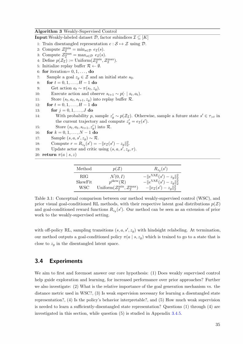
Algorithm 3 Weakly-Supervised Control

Input:Weakly-labeled dataset D, factor subindices I ⊆ [K]

1: Train disentangled representation e : S 7→ Z using D.2: Compute Zmin

I = mins∈D eI(s).3: Compute Zmax

I = maxs∈D eI(s).4: Define p(ZI) := Uniform(Zmin

I ,ZmaxI ).

5: Initialize replay buffer R ← ∅.6: for iteration= 0, 1, . . . , do7: Sample a goal zg ∈ Z and an initial state s0.8: for t = 0, 1, . . . ,H − 1 do9: Get action at ∼ π(st, zg).

10: Execute action and observe st+1 ∼ p(· | st, at).11: Store (st, at, st+1, zg) into replay buffer R.12: for t = 0, 1, . . . ,H − 1 do13: for j = 0, 1, . . . , J do14: With probability p, sample z′g ∼ p(ZI). Otherwise, sample a future state s′ ∈ τ>t in

the current trajectory and compute z′g = eI(s′).

15: Store (st, at, st+1, z′g) into R.

16: for k = 0, 1, . . . , N − 1 do17: Sample (s, a, s′, zg) ∼ R.18: Compute r = Rzg(s

′) = −‖eI(s′)− zg‖22.19: Update actor and critic using (s, a, s′, zg, r).20: return π(a | s, z)

Method p(Z) Rzg(s′)

RIG N (0, I) −‖eVAE(s′)− zg‖22SkewFit pskew(R) −‖eVAE(s′)− zg‖22

WSC Uniform(ZminI ,Zmax

I ) −‖eI(s′)− zg‖22

Table 3.1: Conceptual comparison between our method weakly-supervised control (WSC), andprior visual goal-conditioned RL methods, with their respective latent goal distributions p(Z)and goal-conditioned reward functions Rzg(s

′). Our method can be seen as an extension of priorwork to the weakly-supervised setting.

with off-policy RL, sampling transitions (s, a, s′, zg) with hindsight relabeling. At termination,

our method outputs a goal-conditioned policy π(a | s, zg) which is trained to go to a state that is

close to zg in the disentangled latent space.

3.4 Experiments

We aim to first and foremost answer our core hypothesis: (1) Does weakly supervised control

help guide exploration and learning, for increased performance over prior approaches? Further

we also investigate: (2) What is the relative importance of the goal generation mechanism vs. the

distance metric used in WSC?, (3) Is weak supervision necessary for learning a disentangled state

representation?, (4) Is the policy’s behavior interpretable?, and (5) How much weak supervision

is needed to learn a sufficiently-disentangled state representation? Questions (1) through (4) are

investigated in this section, while question (5) is studied in Appendix 3.4.5.

35

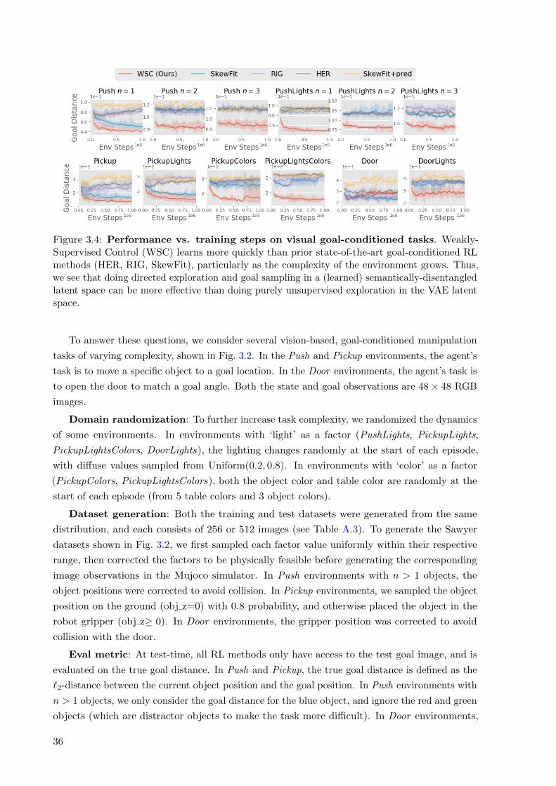
Figure 3.4: Performance vs. training steps on visual goal-conditioned tasks. Weakly-Supervised Control (WSC) learns more quickly than prior state-of-the-art goal-conditioned RLmethods (HER, RIG, SkewFit), particularly as the complexity of the environment grows. Thus,we see that doing directed exploration and goal sampling in a (learned) semantically-disentangledlatent space can be more effective than doing purely unsupervised exploration in the VAE latentspace.

To answer these questions, we consider several vision-based, goal-conditioned manipulation

tasks of varying complexity, shown in Fig. 3.2. In the Push and Pickup environments, the agent’s

task is to move a specific object to a goal location. In the Door environments, the agent’s task is

to open the door to match a goal angle. Both the state and goal observations are 48× 48 RGB

images.

Domain randomization: To further increase task complexity, we randomized the dynamics

of some environments. In environments with ‘light’ as a factor (PushLights, PickupLights,

PickupLightsColors, DoorLights), the lighting changes randomly at the start of each episode,

with diffuse values sampled from Uniform(0.2, 0.8). In environments with ‘color’ as a factor

(PickupColors, PickupLightsColors), both the object color and table color are randomly at the

start of each episode (from 5 table colors and 3 object colors).

Dataset generation: Both the training and test datasets were generated from the same

distribution, and each consists of 256 or 512 images (see Table A.3). To generate the Sawyer

datasets shown in Fig. 3.2, we first sampled each factor value uniformly within their respective

range, then corrected the factors to be physically feasible before generating the corresponding

image observations in the Mujoco simulator. In Push environments with n > 1 objects, the

object positions were corrected to avoid collision. In Pickup environments, we sampled the object

position on the ground (obj z=0) with 0.8 probability, and otherwise placed the object in the

robot gripper (obj z≥ 0). In Door environments, the gripper position was corrected to avoid

collision with the door.

Eval metric: At test-time, all RL methods only have access to the test goal image, and is

evaluated on the true goal distance. In Push and Pickup, the true goal distance is defined as the

`2-distance between the current object position and the goal position. In Push environments with

n > 1 objects, we only consider the goal distance for the blue object, and ignore the red and green

objects (which are distractor objects to make the task more difficult). In Door environments,

36

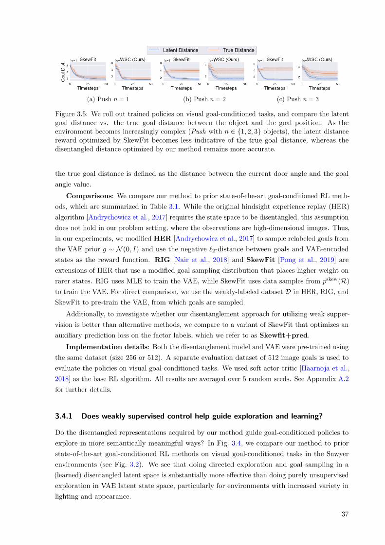
(a) Push n = 1 (b) Push n = 2 (c) Push n = 3

Figure 3.5: We roll out trained policies on visual goal-conditioned tasks, and compare the latentgoal distance vs. the true goal distance between the object and the goal position. As theenvironment becomes increasingly complex (Push with n ∈ {1, 2, 3} objects), the latent distancereward optimized by SkewFit becomes less indicative of the true goal distance, whereas thedisentangled distance optimized by our method remains more accurate.

the true goal distance is defined as the distance between the current door angle and the goal

angle value.

Comparisons: We compare our method to prior state-of-the-art goal-conditioned RL meth-

ods, which are summarized in Table 3.1. While the original hindsight experience replay (HER)

algorithm [Andrychowicz et al., 2017] requires the state space to be disentangled, this assumption

does not hold in our problem setting, where the observations are high-dimensional images. Thus,

in our experiments, we modified HER [Andrychowicz et al., 2017] to sample relabeled goals from

the VAE prior g ∼ N (0, I) and use the negative `2-distance between goals and VAE-encoded

states as the reward function. RIG [Nair et al., 2018] and SkewFit [Pong et al., 2019] are

extensions of HER that use a modified goal sampling distribution that places higher weight on

rarer states. RIG uses MLE to train the VAE, while SkewFit uses data samples from pskew(R)

to train the VAE. For direct comparison, we use the weakly-labeled dataset D in HER, RIG, and

SkewFit to pre-train the VAE, from which goals are sampled.

Additionally, to investigate whether our disentanglement approach for utilizing weak supper-

vision is better than alternative methods, we compare to a variant of SkewFit that optimizes an

auxiliary prediction loss on the factor labels, which we refer to as Skewfit+pred.

Implementation details: Both the disentanglement model and VAE were pre-trained using

the same dataset (size 256 or 512). A separate evaluation dataset of 512 image goals is used to

evaluate the policies on visual goal-conditioned tasks. We used soft actor-critic [Haarnoja et al.,

2018] as the base RL algorithm. All results are averaged over 5 random seeds. See Appendix A.2

for further details.

3.4.1 Does weakly supervised control help guide exploration and learning?

Do the disentangled representations acquired by our method guide goal-conditioned policies to

explore in more semantically meaningful ways? In Fig. 3.4, we compare our method to prior

state-of-the-art goal-conditioned RL methods on visual goal-conditioned tasks in the Sawyer

environments (see Fig. 3.2). We see that doing directed exploration and goal sampling in a

(learned) disentangled latent space is substantially more effective than doing purely unsupervised

exploration in VAE latent state space, particularly for environments with increased variety in

lighting and appearance.

37

Figure 3.6: SkewFit+DR is a variant that samples goals in VAE latent space, but uses rewarddistances in disentangled latent space. We see that the disentangled distance metric can helpslightly in harder environments (e.g., Push n = 3), but the goal generation mechanism of WSCis crucial to achieving efficient exploration.

Then, a natural next question remains: is our disentanglement approach for utilizing weak

supervision better than alternative methods? One obvious approach for using supervision is

to simply add an auxiliary loss to predict the weak labels from the representation. To this

end, we trained a variant of SkewFit where the final hidden layer of the VAE is also trained to

optimize an auxiliary prediction loss on the factor labels, which we refer to as ‘Skewfit+pred’.

In Fig. 3.4, we find that Skewfit+pred performs worse than WSC even though it uses stronger

supervision (exact labels) compared to WSC. Hence, naive auxiliary losses do not lead to good

representations for directing exploration or providing distance metrics. This comparison instead

suggests that our approach of disentangling meaningful and irrelevant factor of the environment

is important for effectively leveraging weak supervision.

3.4.2 Ablation: What is the role of distances vs. goals?

Our method uses the representation in two places: for goal-generation (Eq. 3.2) and for the

distance metric (Eq. 3.3). Our next experiment will study the relative importance of using a

disentangled representation in both places. First, we investigate whether the distance metric

defined over the learned disentangled representation provides a more accurate signal for the true

goal distance. In Fig. 3.5, we evaluate trained policies on visual goal-conditioned tasks, and

compare the latent goal distance vs. the true goal distance between the object and the goal

position at every timestep. As the environment becomes increasingly complex (n ∈ {1, 2, 3}), the

latent distance reward optimized by SkewFit becomes less indicative of the true goal distance

compared to the disentangled distance optimized by our method. The results suggest that the

disentangled representation provide a more accurate reward signal for the training agent.

Next, we tested whether the distance metric in the disentangled space alone is enough to

learn goal-conditioned tasks quickly. To do so, we trained a variant of SkewFit that samples

latent goals in VAE latent space, but uses distances in disentangled latent space as the reward

function. In Fig. 3.6, we see that the disentangled distance metric can help slightly in harder

environments, but underperforms compared to the full method (WSC) with goal generation in

disentangled latent space. Thus, we conclude that both the goal generation mechanism and

distance metric of our method are crucial components for enabling efficient exploration.

38

3.4.3 Is the learned state representation disentangled?

To see whether weak supervision is necessary to learn state representations that are disentangled,

we measure the correlation between true factor values and the latent dimensions of the encoded

image in Table. 3.2. For the VAE, we took the latent dimension that has the highest correlation

with the true factor value. The results illustrate that unsupervised losses are often insufficient

for learning a disentangled representation, and utilizing weak labels in the training process can

greatly improve disentanglement, especially as the environment complexity increases.

Pearson correlationEnv Factor VAE (SkewFit) WSC (Ours)

Pushn = 1

hand x 0.97± 0.04 0.97± 0.01hand y 0.85± 0.07 0.93± 0.02obj x 0.78± 0.28 0.97± 0.01obj y 0.65± 0.31 0.95± 0.01

Pushn = 3

hand x 0.95± 0.03 0.98± 0.01hand y 0.50± 0.33 0.94± 0.03obj1 x 0.12± 0.18 0.96± 0.01obj1 y 0.15± 0.03 0.92± 0.02

Table 3.2: Is the learned state representation disentangled? We measure the correlationbetween the true factor value of the input image vs. the latent dimension of the encoded imageon the evaluation dataset. We show the 95% confidence interval over 5 seeds. We find thatunsupervised VAEs are often insufficient for learning a disentangled representation.

3.4.4 Is the policy’s latent space interpretable?

Since our method uses an interpretable latent goal space to generate self-proposed goals and

compute rewards for training the policy, we checked whether the learned policy is also semantically

meaningful. In Table 3.3, we measure the correlation between latent goals and the final states of

the policy rollout. For various latent goals zg ∈ Z, we rolled out the trained policy π(a | s, zg)and compared the final state with the latent goal zg that the policy was conditioned on (see

Section 3.4.4). For our method, we did a grid sweep over the latent goal values in [ZminI ,Zmax

I ].

For SkewFit, we took the latent dimensions that have the highest correlations with the true object

XY positions, then did a similar grid sweep over the latent goal space. The results show that our

method achieves higher Pearson correlation between latent goals and final states, meaning that

it learns a more interpretable goal-conditioned policy where the latent goals align directly with

the final state of the trajectory rollout.

In Fig. 3.7, we visualize the trajectories generated by our method’s policy when conditioned

on different latent goals zg = (z1, z2) obtained by doing a grid sweep over the latent space

[ZminI ,Zmax

I ]. The object and gripper were spawned at fixed locations at the start of each

trajectory. We see that the latent goal values zg directly align with the final object position after

rolling out the policy π(a | s, zg). In other words, varying each latent goal dimension corresponds

to directly changing the object position in the X- or Y-coordinate. Thus, we conclude that our

method produces a more semantically-meaningful goal-conditioned policy, where the latent goal

39

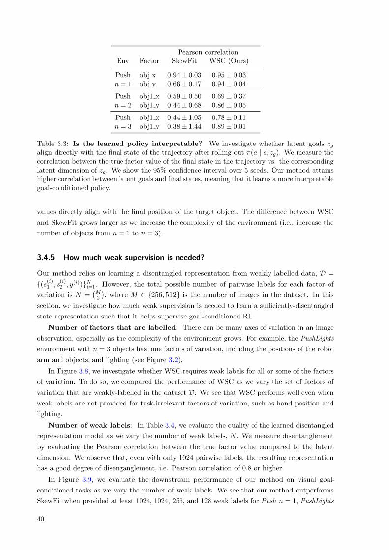
Pearson correlationEnv Factor SkewFit WSC (Ours)

Pushn = 1

obj x 0.94± 0.03 0.95± 0.03obj y 0.66± 0.17 0.94± 0.04

Pushn = 2

obj1 x 0.59± 0.50 0.69± 0.37obj1 y 0.44± 0.68 0.86± 0.05

Pushn = 3

obj1 x 0.44± 1.05 0.78± 0.11obj1 y 0.38± 1.44 0.89± 0.01

Table 3.3: Is the learned policy interpretable? We investigate whether latent goals zgalign directly with the final state of the trajectory after rolling out π(a | s, zg). We measure thecorrelation between the true factor value of the final state in the trajectory vs. the correspondinglatent dimension of zg. We show the 95% confidence interval over 5 seeds. Our method attainshigher correlation between latent goals and final states, meaning that it learns a more interpretablegoal-conditioned policy.

values directly align with the final position of the target object. The difference between WSC

and SkewFit grows larger as we increase the complexity of the environment (i.e., increase the

number of objects from n = 1 to n = 3).

3.4.5 How much weak supervision is needed?

Our method relies on learning a disentangled representation from weakly-labelled data, D =

{(s(i)1 , s

(i)2 , y(i))}Ni=1. However, the total possible number of pairwise labels for each factor of

variation is N =(M2

), where M ∈ {256, 512} is the number of images in the dataset. In this

section, we investigate how much weak supervision is needed to learn a sufficiently-disentangled

state representation such that it helps supervise goal-conditioned RL.

Number of factors that are labelled: There can be many axes of variation in an image

observation, especially as the complexity of the environment grows. For example, the PushLights

environment with n = 3 objects has nine factors of variation, including the positions of the robot

arm and objects, and lighting (see Figure 3.2).

In Figure 3.8, we investigate whether WSC requires weak labels for all or some of the factors

of variation. To do so, we compared the performance of WSC as we vary the set of factors of

variation that are weakly-labelled in the dataset D. We see that WSC performs well even when

weak labels are not provided for task-irrelevant factors of variation, such as hand position and

lighting.

Number of weak labels: In Table 3.4, we evaluate the quality of the learned disentangled

representation model as we vary the number of weak labels, N . We measure disentanglement

by evaluating the Pearson correlation between the true factor value compared to the latent

dimension. We observe that, even with only 1024 pairwise labels, the resulting representation

has a good degree of disenganglement, i.e. Pearson correlation of 0.8 or higher.

In Figure 3.9, we evaluate the downstream performance of our method on visual goal-

conditioned tasks as we vary the number of weak labels. We see that our method outperforms

SkewFit when provided at least 1024, 1024, 256, and 128 weak labels for Push n = 1, PushLights

40

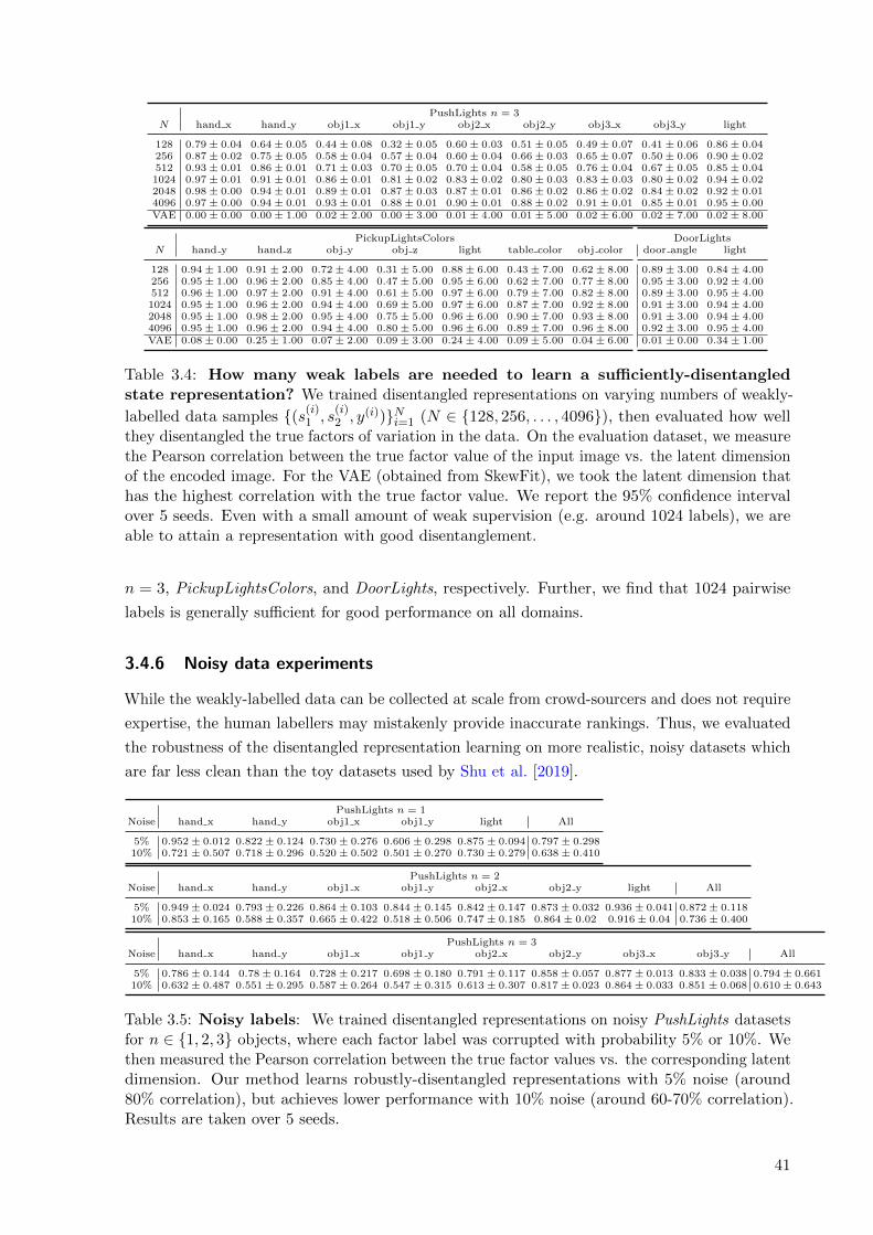
PushLights n = 3N hand x hand y obj1 x obj1 y obj2 x obj2 y obj3 x obj3 y light

128 0.79± 0.04 0.64± 0.05 0.44± 0.08 0.32± 0.05 0.60± 0.03 0.51± 0.05 0.49± 0.07 0.41± 0.06 0.86± 0.04256 0.87± 0.02 0.75± 0.05 0.58± 0.04 0.57± 0.04 0.60± 0.04 0.66± 0.03 0.65± 0.07 0.50± 0.06 0.90± 0.02512 0.93± 0.01 0.86± 0.01 0.71± 0.03 0.70± 0.05 0.70± 0.04 0.58± 0.05 0.76± 0.04 0.67± 0.05 0.85± 0.041024 0.97± 0.01 0.91± 0.01 0.86± 0.01 0.81± 0.02 0.83± 0.02 0.80± 0.03 0.83± 0.03 0.80± 0.02 0.94± 0.022048 0.98± 0.00 0.94± 0.01 0.89± 0.01 0.87± 0.03 0.87± 0.01 0.86± 0.02 0.86± 0.02 0.84± 0.02 0.92± 0.014096 0.97± 0.00 0.94± 0.01 0.93± 0.01 0.88± 0.01 0.90± 0.01 0.88± 0.02 0.91± 0.01 0.85± 0.01 0.95± 0.00VAE 0.00± 0.00 0.00± 1.00 0.02± 2.00 0.00± 3.00 0.01± 4.00 0.01± 5.00 0.02± 6.00 0.02± 7.00 0.02± 8.00

PickupLightsColorsN hand y hand z obj y obj z light table color obj color

128 0.94± 1.00 0.91± 2.00 0.72± 4.00 0.31± 5.00 0.88± 6.00 0.43± 7.00 0.62± 8.00256 0.95± 1.00 0.96± 2.00 0.85± 4.00 0.47± 5.00 0.95± 6.00 0.62± 7.00 0.77± 8.00512 0.96± 1.00 0.97± 2.00 0.91± 4.00 0.61± 5.00 0.97± 6.00 0.79± 7.00 0.82± 8.001024 0.95± 1.00 0.96± 2.00 0.94± 4.00 0.69± 5.00 0.97± 6.00 0.87± 7.00 0.92± 8.002048 0.95± 1.00 0.98± 2.00 0.95± 4.00 0.75± 5.00 0.96± 6.00 0.90± 7.00 0.93± 8.004096 0.95± 1.00 0.96± 2.00 0.94± 4.00 0.80± 5.00 0.96± 6.00 0.89± 7.00 0.96± 8.00VAE 0.08± 0.00 0.25± 1.00 0.07± 2.00 0.09± 3.00 0.24± 4.00 0.09± 5.00 0.04± 6.00

DoorLightsdoor angle light

0.89± 3.00 0.84± 4.000.95± 3.00 0.92± 4.000.89± 3.00 0.95± 4.000.91± 3.00 0.94± 4.000.91± 3.00 0.94± 4.000.92± 3.00 0.95± 4.000.01± 0.00 0.34± 1.00

Table 3.4: How many weak labels are needed to learn a sufficiently-disentangledstate representation? We trained disentangled representations on varying numbers of weakly-

labelled data samples {(s(i)1 , s

(i)2 , y(i))}Ni=1 (N ∈ {128, 256, . . . , 4096}), then evaluated how well

they disentangled the true factors of variation in the data. On the evaluation dataset, we measurethe Pearson correlation between the true factor value of the input image vs. the latent dimensionof the encoded image. For the VAE (obtained from SkewFit), we took the latent dimension thathas the highest correlation with the true factor value. We report the 95% confidence intervalover 5 seeds. Even with a small amount of weak supervision (e.g. around 1024 labels), we areable to attain a representation with good disentanglement.

n = 3, PickupLightsColors, and DoorLights, respectively. Further, we find that 1024 pairwise

labels is generally sufficient for good performance on all domains.

3.4.6 Noisy data experiments

While the weakly-labelled data can be collected at scale from crowd-sourcers and does not require

expertise, the human labellers may mistakenly provide inaccurate rankings. Thus, we evaluated

the robustness of the disentangled representation learning on more realistic, noisy datasets which

are far less clean than the toy datasets used by Shu et al. [2019].

PushLights n = 1Noise hand x hand y obj1 x obj1 y light All

5% 0.952± 0.012 0.822± 0.124 0.730± 0.276 0.606± 0.298 0.875± 0.094 0.797± 0.29810% 0.721± 0.507 0.718± 0.296 0.520± 0.502 0.501± 0.270 0.730± 0.279 0.638± 0.410

PushLights n = 2Noise hand x hand y obj1 x obj1 y obj2 x obj2 y light All

5% 0.949± 0.024 0.793± 0.226 0.864± 0.103 0.844± 0.145 0.842± 0.147 0.873± 0.032 0.936± 0.041 0.872± 0.11810% 0.853± 0.165 0.588± 0.357 0.665± 0.422 0.518± 0.506 0.747± 0.185 0.864± 0.02 0.916± 0.04 0.736± 0.400

PushLights n = 3Noise hand x hand y obj1 x obj1 y obj2 x obj2 y obj3 x obj3 y All

5% 0.786± 0.144 0.78± 0.164 0.728± 0.217 0.698± 0.180 0.791± 0.117 0.858± 0.057 0.877± 0.013 0.833± 0.038 0.794± 0.66110% 0.632± 0.487 0.551± 0.295 0.587± 0.264 0.547± 0.315 0.613± 0.307 0.817± 0.023 0.864± 0.033 0.851± 0.068 0.610± 0.643

Table 3.5: Noisy labels: We trained disentangled representations on noisy PushLights datasetsfor n ∈ {1, 2, 3} objects, where each factor label was corrupted with probability 5% or 10%. Wethen measured the Pearson correlation between the true factor values vs. the corresponding latentdimension. Our method learns robustly-disentangled representations with 5% noise (around80% correlation), but achieves lower performance with 10% noise (around 60-70% correlation).Results are taken over 5 seeds.

41

Real-world dataset: We collected 1,285 RGB images (1,029 train, 256 test) on a real

Franka robot with 5 blocks (see Fig. 3.10a). We collected the images under various indoor lighting

settings and at different times of the day, but we did not provide labels for the environment

lighting conditions. We found that the robot arm often caused occlusion, hiding blocks from

the camera view, so we used two RGB cameras placed at different locations, and stacked the

RGB images into 6 channels (i.e., image arrays of shape 48× 48× 6). We then had a human

provide weak labels for the block positions. In Fig. 3.10b, we show that the learned disentangled

model attains a sufficiently high Pearson correlation between the true XY-position of the block

(relative to the image frame) vs. the corresponding latent dimension of the encoded image. The

results suggest that weakly-supervised disentangled representation learning may be useful for

training robots in the real-world, despite challenges such as environment stochasticity and object

occlusion.

Noisy labels: We generated noisy datasets for PushLights with n ∈ {1, 2, 3} objects, where

each factor label was corrupted with probability 5% or 10%. In Table 3.5, we evaluate the quality

of the learned disentangled representation model on the noisy datasets. Our method learns a

robustly-disentangled representation with 5% noise (around 80% correlation), but achieves lower

performance with 10% noise (around 60-70% correlation).

3.5 Related Work

Reinforcement learning of complex behaviors in rich environments with high-dimensional obser-

vations remains an open problem. Many of the successful applications of RL in prior work [Silver

et al., 2017, Berner et al., 2019, Vinyals et al., 2019, Gu et al., 2017] effectively operate in a

regime where the amount of data (i.e., interactions with the environment) dwarfs the complexity

of task at hand. Insofar as alternative forms of supervision is the key to success for RL methods,

prior work has proposed a number of techniques for making use of various types of ancillary

supervision.

A number of prior works incorporate additional supervision beyond rewards to accelerate

RL. One common theme is to use the task dynamics itself as supervision, using either forward

dynamics [Watter et al., 2015, Finn and Levine, 2017, Hafner et al., 2018, Zhang et al., 2018a,

Kaiser et al., 2019], some function of forward dynamics [Dosovitskiy and Koltun, 2016], or inverse

dynamics [Pathak et al., 2017, Agrawal et al., 2016, Pathak et al., 2018] as a source of labels.

Another approach explicitly predicts auxiliary labels [Jaderberg et al., 2016, Shelhamer et al.,

2016, Gordon et al., 2018, Dilokthanakul et al., 2019]. Compact state representations can also

allow for faster learning and planning, and prior work has proposed a number of tools for learning

these representations [Mahadevan, 2005, Machado et al., 2017, Finn et al., 2016b, Barreto et al.,

2017, Nair et al., 2018, Gelada et al., 2019, Lee et al., 2019a, Yarats et al., 2019]. Bengio et al.

[2017], Thomas et al. [2017] propose learning representations using an independent controllability

metric, but the joint RL and representation learning scheme has proven difficult to scale in

environment complexity. Perhaps most related to our method is prior work that directly learns

a compact representation of goals [Goyal et al., 2019, Pong et al., 2019, Nachum et al., 2018].

Our work likewise learns a low-dimensional representation of goals, but crucially learns it in

42

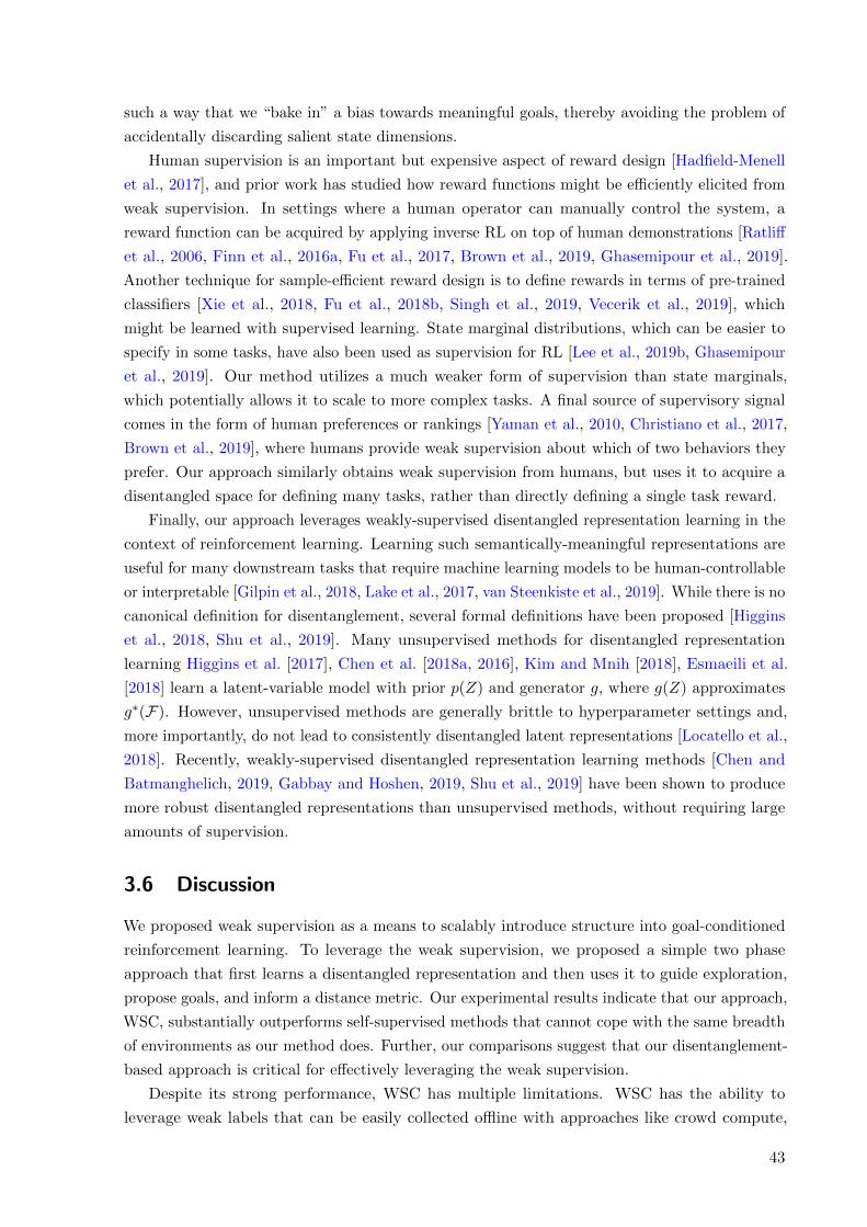
such a way that we “bake in” a bias towards meaningful goals, thereby avoiding the problem of

accidentally discarding salient state dimensions.

Human supervision is an important but expensive aspect of reward design [Hadfield-Menell

et al., 2017], and prior work has studied how reward functions might be efficiently elicited from

weak supervision. In settings where a human operator can manually control the system, a

reward function can be acquired by applying inverse RL on top of human demonstrations [Ratliff

et al., 2006, Finn et al., 2016a, Fu et al., 2017, Brown et al., 2019, Ghasemipour et al., 2019].

Another technique for sample-efficient reward design is to define rewards in terms of pre-trained

classifiers [Xie et al., 2018, Fu et al., 2018b, Singh et al., 2019, Vecerik et al., 2019], which

might be learned with supervised learning. State marginal distributions, which can be easier to

specify in some tasks, have also been used as supervision for RL [Lee et al., 2019b, Ghasemipour

et al., 2019]. Our method utilizes a much weaker form of supervision than state marginals,

which potentially allows it to scale to more complex tasks. A final source of supervisory signal

comes in the form of human preferences or rankings [Yaman et al., 2010, Christiano et al., 2017,

Brown et al., 2019], where humans provide weak supervision about which of two behaviors they

prefer. Our approach similarly obtains weak supervision from humans, but uses it to acquire a

disentangled space for defining many tasks, rather than directly defining a single task reward.

Finally, our approach leverages weakly-supervised disentangled representation learning in the

context of reinforcement learning. Learning such semantically-meaningful representations are

useful for many downstream tasks that require machine learning models to be human-controllable

or interpretable [Gilpin et al., 2018, Lake et al., 2017, van Steenkiste et al., 2019]. While there is no

canonical definition for disentanglement, several formal definitions have been proposed [Higgins

et al., 2018, Shu et al., 2019]. Many unsupervised methods for disentangled representation

learning Higgins et al. [2017], Chen et al. [2018a, 2016], Kim and Mnih [2018], Esmaeili et al.

[2018] learn a latent-variable model with prior p(Z) and generator g, where g(Z) approximates

g∗(F). However, unsupervised methods are generally brittle to hyperparameter settings and,

more importantly, do not lead to consistently disentangled latent representations [Locatello et al.,

2018]. Recently, weakly-supervised disentangled representation learning methods [Chen and

Batmanghelich, 2019, Gabbay and Hoshen, 2019, Shu et al., 2019] have been shown to produce

more robust disentangled representations than unsupervised methods, without requiring large

amounts of supervision.

3.6 Discussion

We proposed weak supervision as a means to scalably introduce structure into goal-conditioned

reinforcement learning. To leverage the weak supervision, we proposed a simple two phase

approach that first learns a disentangled representation and then uses it to guide exploration,

propose goals, and inform a distance metric. Our experimental results indicate that our approach,

WSC, substantially outperforms self-supervised methods that cannot cope with the same breadth

of environments as our method does. Further, our comparisons suggest that our disentanglement-

based approach is critical for effectively leveraging the weak supervision.

Despite its strong performance, WSC has multiple limitations. WSC has the ability to

leverage weak labels that can be easily collected offline with approaches like crowd compute,

43

and does not require human demonstrations or reward specifications, but still may require the

user to indicate the factors of variation that are relevant for downstream tasks. Further, our

method only uses weak supervision during pre-training, which may produce representations that

do not always generalize to new interaction later encountered by the agent. Incorporating weak

supervision online, in the loop of RL, could address this issue to improve performance. In such

settings, we expect class imbalance and human-in-the-loop learning to present important, but

surmountable challenges.

Looking forward, our results suggest a number of interesting directions for future work. For

example, there may be other forms of weak supervision [Shu et al., 2019] that can provide

useful signal to the agent, as well as other ways to leverage these labels. Given the promising

results in increasingly complex environments, evaluating this approach with robots in real-world

environments is an exciting future direction. Overall, we believe that our framework provides a

new perspective on supervising the development of general-purpose agents acting in complex

environments.

The weakly-supervised RL framework utilizes weakly-labelled data to learn a semantically

disentangled representation of images in order to learn more effectively in high-dimensional

task spaces. More generally, language provides a way to encode combinatorial abstractions and

generalizations of the visual and physical world. It also enables us to communicate instructions,

questions, plans, and intentions to one another. How can we utilize language to equip deep RL

agents with structured priors about the physical world, and enable generalization and knowledge

transfer across different tasks? In the next chapter, we consider an embodied navigation agent

that acts in a 3D environment to solve a task specified by an instruction or a question.

44

WSC (Ours) SkewFit

Pu

shn

=1

Pu

shn

=2

Pu

shn

=3

Figure 3.7: Interpretable control: Trajectories generated by WSC (left) and SkewFit (right),where the policies are conditioned on varying latent goals (z1, z2) ∈ R2. For SkewFit, we variedthe latent dimensions that have the highest correlation with the object’s XY-position, and keptthe remaining latent dimensions fixed. The blue object always starts at the center of the framein the beginning of each episode. The white lines indicate the target object’s position throughoutthe trajectory. We see that the disentangled latent goal values of WSC directly align with thedirection in which the WSC policy moves the blue object.

45

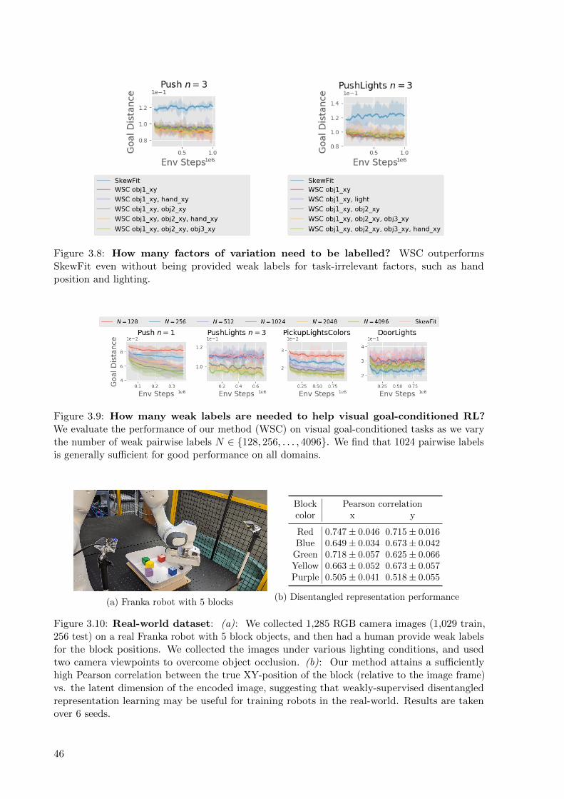
Figure 3.8: How many factors of variation need to be labelled? WSC outperformsSkewFit even without being provided weak labels for task-irrelevant factors, such as handposition and lighting.

Figure 3.9: How many weak labels are needed to help visual goal-conditioned RL?We evaluate the performance of our method (WSC) on visual goal-conditioned tasks as we varythe number of weak pairwise labels N ∈ {128, 256, . . . , 4096}. We find that 1024 pairwise labelsis generally sufficient for good performance on all domains.

(a) Franka robot with 5 blocks

Block Pearson correlationcolor x y

Red 0.747± 0.046 0.715± 0.016Blue 0.649± 0.034 0.673± 0.042

Green 0.718± 0.057 0.625± 0.066Yellow 0.663± 0.052 0.673± 0.057Purple 0.505± 0.041 0.518± 0.055

(b) Disentangled representation performance

Figure 3.10: Real-world dataset: (a): We collected 1,285 RGB camera images (1,029 train,256 test) on a real Franka robot with 5 block objects, and then had a human provide weak labelsfor the block positions. We collected the images under various lighting conditions, and usedtwo camera viewpoints to overcome object occlusion. (b): Our method attains a sufficientlyhigh Pearson correlation between the true XY-position of the block (relative to the image frame)vs. the latent dimension of the encoded image, suggesting that weakly-supervised disentangledrepresentation learning may be useful for training robots in the real-world. Results are takenover 6 seeds.

46

Chapter 4

Multimodal Learning of

Vision, Language and Control

Deep reinforcement learning has been shown to be capable of achieving super-human performance

in playing games such as Atari 2600 [Mnih et al., 2013] and Go [Silver et al., 2016]. Following the

success of deep reinforcement learning in 3D Games such as Doom [Lample and Chaplot, 2017,

Dosovitskiy and Koltun, 2016] and Deepmind Lab [Mnih et al., 2016], there has been increased

interest in using deep reinforcement learning for training embodied AI agents, which interact with

a 3D environment by receiving first-person views of the environment and taking navigational

actions. The simplest navigational agents learn a particular behavior such as collecting or

avoiding particular objects [Kempka et al., 2016, Jaderberg et al., 2016, Mirowski et al., 2016] or

playing deathmatches [Lample and Chaplot, 2017, Dosovitskiy and Koltun, 2016]. Subsequently,

there have been efforts on training navigational agents whose behavior is conditioned on a

target specified using images [Zhu et al., 2017] or coordinates [Gupta et al., 2017a, Savva et al.,

2017]. More recently, there has been much interest in training agents with goals specified (either

explicitly or implicitly) via language since that offers several advantages over using images or

coordinates.

First, the compositional structure of language allows generalization to new tasks without

additional learning. Prior work [Oh et al., 2017, Hermann et al., 2017, Chaplot et al., 2017] has

trained navigational agents to follow instructions and shown zero-shot generalization to new

instructions which contain unseen composition of words seen in the training instructions. Second,

language is also a natural means for humans to communicate with autonomous agents. Language

not only allows instruction but also interaction. Gordon et al. [2018] and Das et al. [2017] train

agents to answer questions by navigating in the environment to gather the required information.

Figure 4.1a shows examples of these multimodal tasks. The agent interacts with the envi-

ronment by receiving pixel-level visual input and an instruction or a question specifying the

task. These multimodal tasks involve several challenges including perception from raw pixels,

grounding of words in the instruction or question to visual objects and attributes, reasoning

to perform relational tasks, fine-grained navigation in 3D environments with continuous state

space, and learning to answer questions. Training a model for each task typically requires tens

or hundreds of millions of frames. In this paper, we train a multi-task navigation model to

follow instructions and answer questions. Training a single model to perform multiple tasks

47

can help improve the sample efficiency as many of the aforementioned challenges are common

between different multimodal tasks. Furthermore, training a multi-task model can also facilitate

knowledge transfer between the tasks and allow the model to generalize to scenarios which were

not possible with single tasks. For example, if an agent learns to follow the instruction ‘Go to

the red torch’ and answer the question ‘What color is the pillar?’, then ideally it should also be

able to follow the instruction ‘Go to the red pillar’ and answer the question ‘What color is the

torch?’ without any additional training.

Consequently, we define cross-task knowledge transfer evaluation criterion to test the general-

ization ability of multimodal multi-task models. This criterion evaluates zero-shot learning on

instructions and questions consisting of unseen composition of words in both tasks. In order to

achieve cross-task knowledge transfer, words in the input space of both tasks need to be aligned

with each other and with the answer space while they are being grounded to visual objects and

attributes. In the above example, in order to answer the question ‘What color is the pillar?’, the

knowledge of the word ‘pillar’ and its grounding in the visual world must be transferred from

instructions, as it is never seen in any training question. Also, the agent also needs to learn to

relate the word ‘red’ in the input space with the answer ‘red’ along with its grounding in the

visual world.

There has been work on training single-task models for both instruction following and

embodied question answering. We show that several prior single-task models, when trained on

both tasks, fail to achieve cross-task knowledge transfer. In the above example, if the model sees

the word ‘pillar’ only in instructions during training, its representation of the word ‘pillar’ would

be associated with the instruction following task. Consequently, it would always take navigational

actions whenever it sees the word ‘pillar’ in a test question and never any answer actions.

We propose a novel dual-attention model involving sequential Gated- and Spatial-Attention

operations to perform explicit task-invariant alignment between the image representation channels

and the words in the input and answer space. We create datasets and simulation scenarios for

testing cross-task knowledge transfer in the Doom environment [Kempka et al., 2016] and show

an absolute improvement of 43-61% on instructions and 5-26% for questions over baselines in a

range of scenarios with varying difficulty. Additionally, we demonstrate that the modularity of

our model allows easy addition of new objects and attributes to a trained model.

4.1 Related Work

This paper is motivated by a series of works on learning to follow navigation instructions [Oh

et al., 2017, Hermann et al., 2017, Chaplot et al., 2017, Wu et al., 2018, Yu et al., 2018a] and

learning to answer questions by navigating around the environment [Das et al., 2017, Gordon

et al., 2018]. Among methods learning from instructions in 3D environments, Oh et al. [2017]

introduced a hierarchical RL model for learning sequences of instructions by learning skills to

solve subtasks. Chaplot et al. [2017] introduced a gated-attention model for multimodal fusion

of textual and visual representations using multiplicative interactions, whereas Hermann et al.

[2017] introduced auxiliary tasks such as temporal autoencoding and language prediction to

improve sample efficiency for this task. Yu et al. [2018a] proposed guided feature transformation

48

(a) Embodied multimodal tasks (b) Bird’s eye view of the map

Figure 4.1: (a) We consider embodied multimodal tasks, where the agent receives visual first-person observations and an instruction or a question specifying the task. (b) Example startingstates and bird’s eye view of the map showing agent and candidate object locations in Easy andHard settings.

which transforms visual representations using latent sentence embeddings computed from the

language input.

Among models for embodied question answering, Das et al. [2017] introduced a hierarchical

model consisting of 4 modules, each for processing images, encoding questions, navigation, and

question-answering, each of which is pretrained with supervised or imitation learning, followed

by fine-tuning of the navigation model using reinforcement learning. Gordon et al. [2018]

introduced the task of Interactive Question Answering which involves interacting with objects

in the environment with non-navigational actions for answering questions. They proposed

Hierarchical Interactive Memory Network (HIMN), which allows temporal abstraction using a

factorized set of controllers.

All of the above methods are designed for a single task, following navigational instructions

or answering questions, whereas we train a single model for both tasks. Yu et al. [2018b]

introduced a model for interactive language acquisition by training on both Visual Question

Answering and following instructions in a 2D grid world environment. In contrast, we tackle

multimodal multitask learning in challenging 3D environments. Partial observability results in

the requirement of learning to navigate for answering the questions, turning visual question

answering to embodied question answering. 3D environments also allow us to test interesting and

more challenging instructions, such as those based on the relative size of the objects, in addition

to object types and colors.

In addition to the above, there is a large body of work on multimodal learning in static

settings which do not involve navigation or reinforcement learning. Some relevant works which

use attention mechanisms similar to the ones used in our proposed model include Perez et al.

[2017], Fukui et al. [2016], Xu and Saenko [2016], Hudson and Manning [2018], Gupta et al.

[2017b] for Visual Question Answering and Zhao et al. [2018] for grounding audio to vision.

49

Table 4.1: Table showing training and test sets for both Semantic Goal Navigation (SGN) andEmbodied Question Answering (EQA) tasks. The test set consists of unseen instructions andquestions. The dataset evaluates a model for cross-task knowledge transfer between SGN andEQA.

Task Train Set Test Set

SGN Instructions NOT containing ‘red’ & ‘pillar’: Instructions containing ‘red’ or ‘pillar’:‘Go to the largest blue object’ ‘Go to the red pillar’‘Go to the torch’ ‘Go to the tall red object’

EQA Questions NOT containing ‘blue’ & ‘torch’: Questions containing ‘blue’ or ‘torch’:‘Which is the smallest red object?’ ‘Which object is blue in color?’‘What color is the tall pillar?’ ‘What color is the torch?’

4.2 Problem Formulation

Consider an autonomous agent interacting with an episodic environment as shown in Figure 4.1.

At the beginning of each episode, the agent receives a textual input T specifying the task that

it needs to achieve. For example, T could be an instruction asking to navigate to the target

object or a question querying some visual detail of objects in the environment. At each time

step t, the agent observes a state st = (It, T ) where It is the first-person (egocentric) view of the

environment, and takes an action at, which could be a navigational action or an answer action.

The agent’s objective is to learn a policy π(at|st) which leads to successful completion of the

task specified by the textual input T .

Tasks. We focus on the multi-task learning of two visually-grounded language navigation

tasks: In Embodied Question Answering (EQA), the agent is given a question (‘What color is the

torch?’), and it must navigate around the 3D environment to explore the environment and gather

information to answer the question (‘red’). In Semantic Goal Navigation (SGN), the agent is

given a language instruction (‘Go to the red torch’) to navigate to a goal location.

Environments. We adapt the ViZDoom [Kempka et al., 2016]-based language grounding

environment proposed by Chaplot et al. [2017] for visually-grounded multitask learning. It

consists of a single room with 5 objects. The objects are randomized in each episode based on

the textual input. We use two difficulty settings for the Doom domain as shown in Figure 4.1b:

Easy : The agent is spawned at a fixed location. The candidate objects are spawned at five fixed

locations along a single horizontal line in the field of view of the agent. Hard : The candidate

objects and the agent are spawned at random locations and the objects may or may not be in

the agent’s field of view in the initial configuration. The agent must explore the map to view all

objects. The agent can take 4 actions: 3 navigational actions (forward, left, right) and 1 answer

action. When the agent takes the answer action, the answer with the maximum probability in

the output answer distribution is used.

Datasets. We use the set of 70 instructions from Chaplot et al. [2017] and create a

dataset for 29 questions using the same set of objects and attributes. These datasets include

instructions and questions about object types, colors, relative sizes (tall/short) and superlative

sizes (smallest/largest). We define cross-task knowledge transfer as an evaluation criterion for

testing the generalization of multi-task models. We create train-test splits for both instructions

and questions datasets to explicitly test a multitask model’s ability to transfer the knowledge of

50

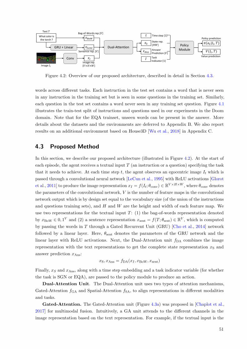
𝑥"#$

𝑥%Image rep. [𝑉×𝐻×𝑊]

Bag-of-Words rep.[𝑉]

𝑥*+,-Sentence rep. [𝑉]

Conv

Dual-Attention

What color is the torch ?

GRU + Linear

Image 𝐼-

Text 𝑇

𝑥1,2 Answer Prediction [𝑉]

𝑥* State rep. [𝐻𝑊] Policy

Module

𝑡 Time step [1]

𝐼 Task Indicator [1]

𝑉(𝐼-, 𝑇)

𝜋(𝑎-|𝐼-, 𝑇)Policy prediction

Value prediction

Figure 4.2: Overview of our proposed architecture, described in detail in Section 4.3.

words across different tasks. Each instruction in the test set contains a word that is never seen

in any instruction in the training set but is seen in some questions in the training set. Similarly,

each question in the test set contains a word never seen in any training set question. Figure 4.1

illustrates the train-test split of instructions and questions used in our experiments in the Doom

domain. Note that for the EQA trainset, unseen words can be present in the answer. More

details about the datasets and the environments are deferred to Appendix B. We also report

results on an additional environment based on House3D [Wu et al., 2018] in Appendix C.

4.3 Proposed Method

In this section, we describe our proposed architecture (illustrated in Figure 4.2). At the start of

each episode, the agent receives a textual input T (an instruction or a question) specifying the task

that it needs to achieve. At each time step t, the agent observes an egocentric image It which is

passed through a convolutional neural network [LeCun et al., 1995] with ReLU activations [Glorot

et al., 2011] to produce the image representation xI = f(It; θconv) ∈ RV×H×W , where θconv denotes

the parameters of the convolutional network, V is the number of feature maps in the convolutional

network output which is by design set equal to the vocabulary size (of the union of the instructions

and questions training sets), and H and W are the height and width of each feature map. We

use two representations for the textual input T : (1) the bag-of-words representation denoted

by xBoW ∈ 0, 1V and (2) a sentence representation xsent = f(T ; θsent) ∈ RV , which is computed

by passing the words in T through a Gated Recurrent Unit (GRU) [Cho et al., 2014] network

followed by a linear layer. Here, θsent denotes the parameters of the GRU network and the

linear layer with ReLU activations. Next, the Dual-Attention unit fDA combines the image

representation with the text representations to get the complete state representation xS and

answer prediction xAns:

xS, xAns = fDA(xI , xBoW, xsent)

Finally, xS and xAns, along with a time step embedding and a task indicator variable (for whether

the task is SGN or EQA), are passed to the policy module to produce an action.

Dual-Attention Unit. The Dual-Attention unit uses two types of attention mechanisms,

Gated-Attention fGA and Spatial-Attention fSA, to align representations in different modalities

and tasks.

Gated-Attention. The Gated-Attention unit (Figure 4.3a) was proposed in [Chaplot et al.,

2017] for multimodal fusion. Intuitively, a GA unit attends to the different channels in the

image representation based on the text representation. For example, if the textual input is the

51

(a) Gated-Attention unit fGA (b) Spatial-Attention unit fSA

Figure 4.3: The Dual-Attention unit uses two types of attention mechanisms (a, b) to alignrepresentations in different modalities and tasks.

instruction ‘Go to the red pillar’, then the GA unit can learn to attend to channels which detect

red things and pillars. Specifically, the GA unit takes as input a 3-dimensional tensor image

representation yI ∈ Rd×H×W and a text representation yT ∈ Rd, and outputs a 3-dimensional

tensor z ∈ Rd×H×W 1. Note that the dimension of yT is equal to the number of feature maps

and the size of the first dimension of yI . In the Gated-Attention unit, each element of yT

is expanded to a H ×W matrix, resulting in a 3-dimensional tensor MyT ∈ Rd×H×W , whose

(i, j, k)th element is given by MyT [i, j, k] = yT [i]. This matrix is multiplied element-wise with

the image representation: z = fGA(yI , yT ) = MyT � yI , where � denotes the Hadamard product

[Horn, 1990].

Spatial-Attention. We propose a Spatial-Attention unit (Figure 4.3b) which is analogous

to the Gated-Attention unit except that it attends to different pixels in the image representation

rather than the channels. For example, if the textual input is the question ‘Which object is

blue in color?’, then we would like to spatially attend to the parts of the image which contain a

blue object in order recognize the type of the blue object. The Spatial-Attention unit takes as

input a 3-dimensional tensor image representation yI ∈ Rd×H×W and a 2-dimensional spatial

attention map yS ∈ RH×W , and outputs a tensor z ∈ Rd×H×W . Note that the height and

width of the spatial attention map is equal to the height and width of the image representation.

In the spatial-attention unit, each element of the spatial attention map is expanded to a d

dimensional vector. This again results in a 3-dimensional tensor MyS ∈ Rd×H×W , whose (i, j, k)th

element is given by: MyS [i, j, k] = yS [j, k]. Just like in the Gated-Attention unit, this matrix

is multiplied element-wise with the image representation: z = fSA(yI , yS) = MyS � yI . Similar

spatial attention mechanisms have been used for Visual Question Answering [Fukui et al., 2016,

Xu and Saenko, 2016, Hudson and Manning, 2018, Gupta et al., 2017b] and grounding audio in

vision [Zhao et al., 2018].

Dual-Attention. We now describe the operations in the Dual-Attention unit shown in

Figure 4.4, as well as motivate the intuitions behind each operation. Given xI , xBoW, and xsent,

the Dual-Attention unit first computes a Gated-Attention over xI using xBoW:

xGA1 = fGA(xI , xBoW) ∈ RV×H×W . (4.1)

Intuitively, this first Gated-Attention unit grounds each word in the vocabulary with a feature

1We use the variables y and z to describe the Gated-Attention and Spatial-Attention units in a general capacity.We will later instantiate these units multiple times with x variables in our model.

52

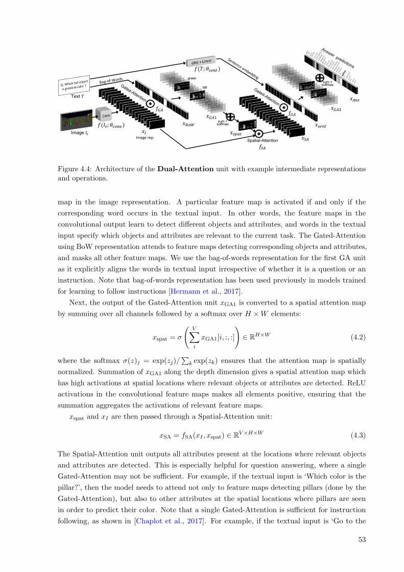
Gated-Attention

sum +softmax

Spatial-Attention𝑓"#

Answer predictions

tall

greensum +

softmaxBag-of-Words

Sentence embedding

𝑥%𝑥&'(

𝑥)#*

Gated-Attention

Image rep.

𝑥+,-.

𝑥"#𝑥+/0.

𝑥)#1

𝑥#-+

𝑓(𝐼.; 𝜃6'-7)

𝑓(𝑇; 𝜃+,-. )

Image 𝐼.

Text 𝑇

𝑓)# 𝑓)#

Figure 4.4: Architecture of the Dual-Attention unit with example intermediate representationsand operations.

map in the image representation. A particular feature map is activated if and only if the

corresponding word occurs in the textual input. In other words, the feature maps in the

convolutional output learn to detect different objects and attributes, and words in the textual

input specify which objects and attributes are relevant to the current task. The Gated-Attention

using BoW representation attends to feature maps detecting corresponding objects and attributes,

and masks all other feature maps. We use the bag-of-words representation for the first GA unit

as it explicitly aligns the words in textual input irrespective of whether it is a question or an

instruction. Note that bag-of-words representation has been used previously in models trained

for learning to follow instructions [Hermann et al., 2017].

Next, the output of the Gated-Attention unit xGA1 is converted to a spatial attention map

by summing over all channels followed by a softmax over H ×W elements:

xspat = σ

(V∑i

xGA1[i, :, :]

)∈ RH×W (4.2)

where the softmax σ(z)j = exp(zj)/∑

k exp(zk) ensures that the attention map is spatially

normalized. Summation of xGA1 along the depth dimension gives a spatial attention map which

has high activations at spatial locations where relevant objects or attributes are detected. ReLU

activations in the convolutional feature maps makes all elements positive, ensuring that the

summation aggregates the activations of relevant feature maps.

xspat and xI are then passed through a Spatial-Attention unit:

xSA = fSA(xI , xspat) ∈ RV×H×W (4.3)

The Spatial-Attention unit outputs all attributes present at the locations where relevant objects

and attributes are detected. This is especially helpful for question answering, where a single

Gated-Attention may not be sufficient. For example, if the textual input is ‘Which color is the

pillar?’, then the model needs to attend not only to feature maps detecting pillars (done by the

Gated-Attention), but also to other attributes at the spatial locations where pillars are seen

in order to predict their color. Note that a single Gated-Attention is sufficient for instruction

following, as shown in [Chaplot et al., 2017]. For example, if the textual input is ‘Go to the

53

green pillar’, the first Gated-Attention unit can learn to attend to feature maps detecting green

objects and pillar, and learn a navigation policy based on the spatial locations of the feature

map activations.

xSA is then passed through another Gated-Attention unit with the sentence-level text repre-

sentation:

xGA2 = fGA(xSA, xsent) ∈ RV×H×W (4.4)

This second Gated-Attention unit enables the model to attend to different types of attributes

based on the question. For instance, if the question is asking about the color (‘Which color is

the pillar?’), then the model needs to attend to the feature maps corresponding to colors; or if

the question is asking about the object type (‘Which object is green in color?’), then the model

needs to attend to the feature maps corresponding to object types. The sentence embedding

xsent can learn to attend to multiple channels based on the textual input and mask the rest.

Next, the output is transformed to answer prediction by again doing a summation and

softmax but this time summing over the height and width instead of the channels:

xAns = σ

H,W∑j,k

xGA2[:, j, k]

∈ RV (4.5)

Summation of xGA2 along each feature map aggregates the activations for relevant attributes

spatially. Again, ReLU activations for sentence embedding ensure aggregation of activations for

each attribute or word. The answer space is identical to the textual input space RV .

Finally, the Dual-Attention unit fDA outputs the answer prediction xAns and the flattened

spatial attention map xS = vec(xspat), where vec(·) denotes the flattening operation.

Policy Module. The policy module takes as input the state representation xS from the

Dual-Attention unit, a time step embedding t, and a task indicator variable I (for whether the

task is SGN or EQA). The inputs are concatenated then passed through a linear layer, then a

recurrent GRU layer, then linear layers to estimate the policy function π(at | It, T ) and the value

function V (It, T ).

All above operations are differentiable, making the entire architecture trainable end-to-end.

Note that all attention mechanisms in the Dual-Attention unit only modulate the input image

representation, i.e., mask or amplify specific feature maps or pixels. This ensures that there is

an explicit alignment between the words in the textual input, the feature maps in the image

representation, and the words in answer space. This forces the convolutional network to encode

all the information required with respect to a certain word in the corresponding output channel.

For the model to predict ‘red’ as the answer, it must detect red objects in the corresponding

feature map. This explicit task-invariant alignment between convolutional feature maps and

words in the input and answer space facilitates grounding and allows for cross-task knowledge

transfer. As shown in the results later, this also makes our model modular and allows easy

addition of objects and attributes to a trained model.

Optimization. The entire model is trained to predict both navigational actions and answers

jointly. The policy is trained using Proximal Policy Optimization (PPO) [Schulman et al., 2017].

For training the answer predictions, we use a supervised cross-entropy loss. Both types of losses

have common parameters as the answer prediction is essentially an intermediate representation

for the policy.

54

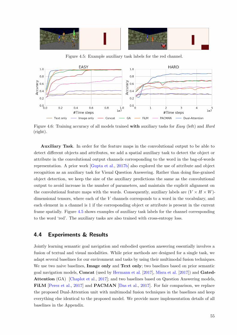
Figure 4.5: Example auxiliary task labels for the red channel.

Figure 4.6: Training accuracy of all models trained with auxiliary tasks for Easy (left) and Hard(right).

Auxiliary Task. In order for the feature maps in the convolutional output to be able to

detect different objects and attributes, we add a spatial auxiliary task to detect the object or

attribute in the convolutional output channels corresponding to the word in the bag-of-words

representation. A prior work [Gupta et al., 2017b] also explored the use of attribute and object

recognition as an auxiliary task for Visual Question Answering. Rather than doing fine-grained

object detection, we keep the size of the auxiliary predictions the same as the convolutional

output to avoid increase in the number of parameters, and maintain the explicit alignment on

the convolutional feature maps with the words. Consequently, auxiliary labels are (V ×H ×W )-

dimensional tensors, where each of the V channels corresponds to a word in the vocabulary, and

each element in a channel is 1 if the corresponding object or attribute is present in the current

frame spatially. Figure 4.5 shows examples of auxiliary task labels for the channel corresponding

to the word ‘red’. The auxiliary tasks are also trained with cross-entropy loss.

4.4 Experiments & Results

Jointly learning semantic goal navigation and embodied question answering essentially involves a

fusion of textual and visual modalities. While prior methods are designed for a single task, we

adapt several baselines for our environment and tasks by using their multimodal fusion techniques.

We use two naive baselines, Image only and Text only; two baselines based on prior semantic

goal navigation models, Concat (used by Hermann et al. [2017], Misra et al. [2017]) and Gated-

Attention (GA) [Chaplot et al., 2017]; and two baselines based on Question Answering models,

FiLM [Perez et al., 2017] and PACMAN [Das et al., 2017]. For fair comparison, we replace

the proposed Dual-Attention unit with multimodal fusion techniques in the baselines and keep

everything else identical to the proposed model. We provide more implementation details of all

baselines in the Appendix.

55

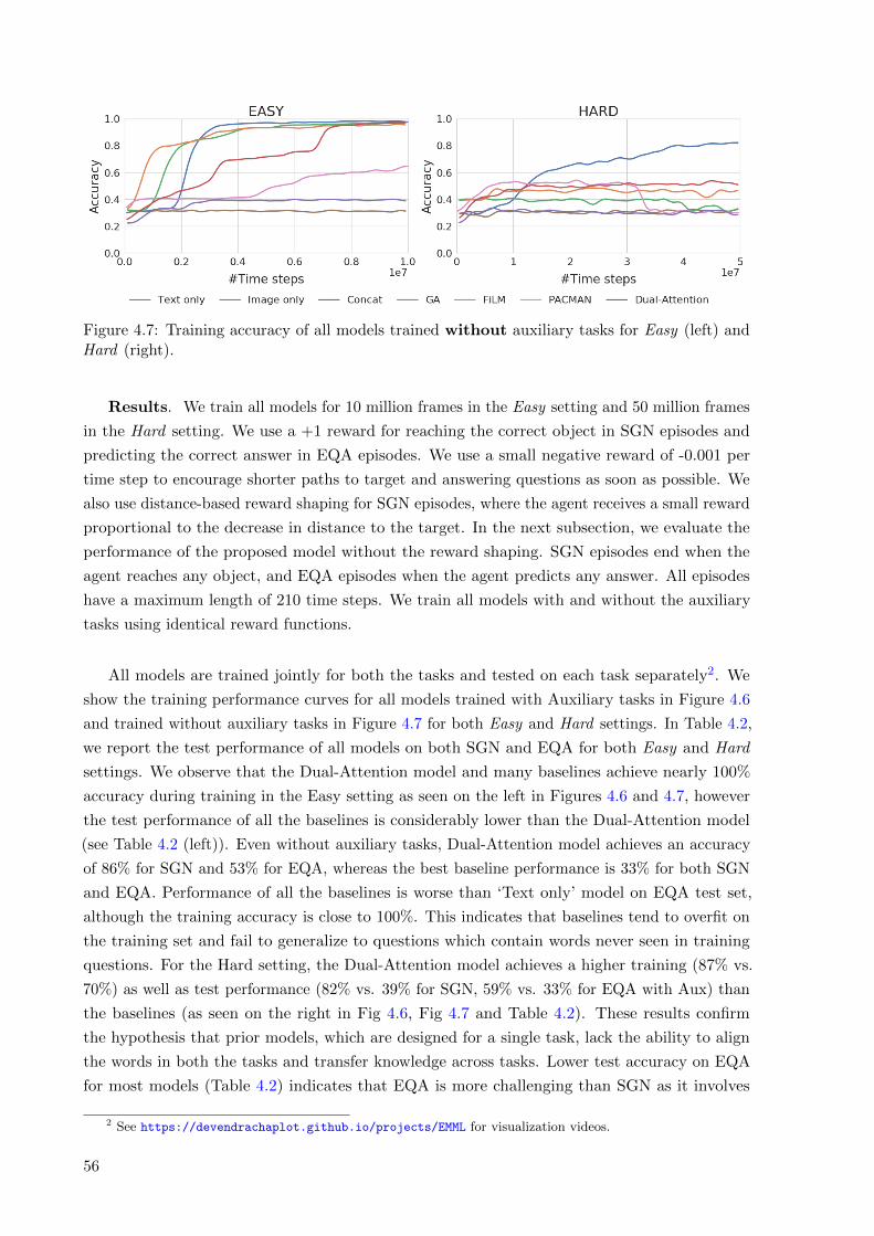
Figure 4.7: Training accuracy of all models trained without auxiliary tasks for Easy (left) andHard (right).

Results. We train all models for 10 million frames in the Easy setting and 50 million frames

in the Hard setting. We use a +1 reward for reaching the correct object in SGN episodes and

predicting the correct answer in EQA episodes. We use a small negative reward of -0.001 per

time step to encourage shorter paths to target and answering questions as soon as possible. We

also use distance-based reward shaping for SGN episodes, where the agent receives a small reward

proportional to the decrease in distance to the target. In the next subsection, we evaluate the

performance of the proposed model without the reward shaping. SGN episodes end when the

agent reaches any object, and EQA episodes when the agent predicts any answer. All episodes

have a maximum length of 210 time steps. We train all models with and without the auxiliary

tasks using identical reward functions.

All models are trained jointly for both the tasks and tested on each task separately2. We

show the training performance curves for all models trained with Auxiliary tasks in Figure 4.6

and trained without auxiliary tasks in Figure 4.7 for both Easy and Hard settings. In Table 4.2,

we report the test performance of all models on both SGN and EQA for both Easy and Hard

settings. We observe that the Dual-Attention model and many baselines achieve nearly 100%

accuracy during training in the Easy setting as seen on the left in Figures 4.6 and 4.7, however

the test performance of all the baselines is considerably lower than the Dual-Attention model

(see Table 4.2 (left)). Even without auxiliary tasks, Dual-Attention model achieves an accuracy

of 86% for SGN and 53% for EQA, whereas the best baseline performance is 33% for both SGN

and EQA. Performance of all the baselines is worse than ‘Text only’ model on EQA test set,

although the training accuracy is close to 100%. This indicates that baselines tend to overfit on

the training set and fail to generalize to questions which contain words never seen in training

questions. For the Hard setting, the Dual-Attention model achieves a higher training (87% vs.

70%) as well as test performance (82% vs. 39% for SGN, 59% vs. 33% for EQA with Aux) than

the baselines (as seen on the right in Fig 4.6, Fig 4.7 and Table 4.2). These results confirm

the hypothesis that prior models, which are designed for a single task, lack the ability to align

the words in both the tasks and transfer knowledge across tasks. Lower test accuracy on EQA

for most models (Table 4.2) indicates that EQA is more challenging than SGN as it involves

2 See https://devendrachaplot.github.io/projects/EMML for visualization videos.

56

Table 4.2: Accuracy of all models on SGN & EQA test sets for both Easy & Hard difficulties.

Easy HardNo Aux Aux No Aux Aux

Model SGN EQA SGN EQA SGN EQA SGN EQA

Text only 0.2 0.33 0.2 0.33 0.2 0.33 0.2 0.33Image only 0.20 0.09 0.21 0.08 0.16 0.08 0.15 0.08Concat 0.33 0.21 0.31 0.19 0.2 0.26 0.39 0.22GA 0.27 0.18 0.35 0.24 0.18 0.11 0.22 0.24FiLM 0.24 0.11 0.34 0.12 0.12 0.03 0.25 0.15PACMAN 0.26 0.12 0.33 0.10 0.29 0.33 0.11 0.27Dual-Attention 0.86 0.53 0.96 0.58 0.86 0.38 0.82 0.59

alignment between not only input textual and visual representations but also with the answer

space. As expected, using spatial auxiliary tasks lead to better performance for all models

(Table 4.2).

Visualizations. Figure 4.9 shows an example indicating that the sentence-level embedding

for the question attends to relevant words. It also shows a visualization of spatial-attention maps

and answer predictions for each frame in an example EQA episode. The spatial attention map

shows that the model attends to relevant objects and attributes based on the question. The

answer predictions change as the agent views more objects. These visualizations show that the

textual and visual representations are aligned with each other, as well as with the answer space,

as expected. In Figure 4.8, we visualize the convolutional network outputs corresponding to

7 words for the same frame for both Aux and No Aux models. As expected, the Aux model

predictions are very close to the auxiliary task labels. More interestingly, the convolutional

outputs of the No Aux model show that words and objects/properties in the images have been

properly aligned even when the model is not trained with any auxiliary task labels.2

4.4.1 Ablation tests

We perform a series of ablation tests in order to analyze the contribution of each component in

the Dual-Attention unit: without Spatial-Attention (w/o SA), without the first Gated-Attention

with xBoW (w/o GA1), and without the second Gated-Attention with xsent (w/o GA2). We

also try removing the task indicator variable (w/o Indicator Variable), removing reward

shaping (w/o Reward Shaping), and training the proposed model on a single task, SGN or

EQA (DA Single-Task).

Figure 4.10 shows the training performance curves for the Dual-Attention model along with

all ablation models in the Easy Setting. In Table 4.3, we report the test set performance of all

ablation models. The results indicate that SA and GA1 contribute the most to the performance of

the Dual-Attention model. GA2 is critical for performance on EQA but not SGN (see Table 4.3).

This is expected as GA2 is designed to attend to different objects and attributes based on the

question and is used mainly for answer prediction. It is not critical for SGN as the spatial

attention map consists of locations of relevant objects, which is sufficient for navigating to the

correct object. Reward shaping and indicator variable help with learning speed (see Figure 4.10),

but have little effect on the final performance (see Table 4.3). Dual-Attention models trained

57

Figure 4.8: Visualizations of convolutional output channels. We visualize the convolutionalchannels corresponding to 7 words (one in each row) for the same frame (shown in the rightmostcolumn). The first column shows the auxiliary task labels for reference. The second column andthird column show the output of the corresponding channel for the proposed Dual-Attentionmodel trained without and with auxiliary tasks, respectively. As expected, the Aux modeloutputs are very close to the auxiliary task labels. The convolutional outputs of the No Auxmodel show that words and objects/properties in the images have been properly aligned evenwhen the model is not trained with any auxiliary task labels. We do not provide any auxiliarylabel for words ‘smallest’ and ‘largest’ as they are not properties of an object and require relativecomparison of objects. The visualizations in row 5 (corresponding to ‘smallest’) indicate thatboth models are able to compare the sizes of objects and detect the smallest object in thecorresponding output channel even without any aux labels for the smallest object.

58

Figure 4.9: Spatial Attention and Answer Prediction Visualizations. An example EQAepisode with the question “Which is the smallest blue object?”. The sentence embedding ofthe question is shown on the top (xsent). As expected, the embedding attends to object typewords (’torch’, ’pillar’, ’skullkey’, etc.) as the question is asking about an object type (’Whichobject’). The rows show increasing time steps and columns show the input frame, the inputframe overlaid with the spatial attention map, the predicted answer distribution, and the actionat each time step. As the agent is turning, the spatial attention attends to small and blueobjects. Time steps 1, 2: The model is attending to the yellow skullkey but the probability ofthe answer is not sufficiently high, likely because the skullkey is not blue. Time step 3: Themodel cannot see the skullkey anymore so it attends to the armor which is next smallest object.Consequently, the answer prediction also predicts armor, but the policy decides not to answerdue to low probability. Time step 4: As the agent turns more, it observes and attends to theblue skullkey. The answer prediction for ‘skullkey’ has high probability because it is small andblue, so the policy decides to answer the question.

only on single tasks work well on SGN, especially with auxiliary tasks. This is because the

auxiliary task for single task models includes object detection labels corresponding to the words

in the test set. This highlights a key advantage of the proposed model. Due to its modular

and interpretable design, the model can be used for transferring the policy to new objects and

attributes without fine-tuning as discussed in the following subsection.

4.4.2 Extension: Transfer to new words

Consider a scenario of SGN where the agent is trained to follow instructions of certain objects and

attributes. Suppose that the user wants the agent to follow instructions about a new object such

as ‘pillar’ or a new attribute such the color ‘red’ which are never seen in any training instruction.

Prior SGN models are shown to perform well to unseen combination of object-attribute pairs

[Chaplot et al., 2017], but they do not generalize well to instructions containing a new word.

The model retrained only on new instructions will lead to catastrophic forgetting of previous

59

Figure 4.10: Training accuracy of proposed Dual-Attention model with all ablation modelstrained without (left) and with (right) auxiliary tasks for the Easy environment.

Table 4.3: Accuracy of all the ablation modelstrained with and without Auxiliary tasks onSGN and EQA test sets for the Doom Easyenvironment.

No Aux AuxModel SGN EQA SGN EQA

w/o SA 0.20 0.16 0.20 0.15w/o GA1 0.14 0.25 0.16 0.38w/o GA2 0.80 0.33 0.97 0.15w/o Task Indicator 0.79 0.47 0.96 0.56w/o Reward Shaping 0.82 0.49 0.93 0.51DA Single-Task 0.63 0.31 0.91 0.34DA Multi-Task 0.86 0.53 0.96 0.58

Table 4.4: The performance of a trained pol-icy appended with object detectors on instruc-tions containing unseen words (‘red’ and ‘pil-lar’).

Instruction Easy Hard

Go to the pillar 1.00 0.71Go to the red object 0.99 0.89Go to the tall/short pillar 0.99 0.68Go to the <known color>pillar. 1.00 0.79Go to the red <known object> 1.00 0.93Go to the largest/smallest red object 0.95 0.69Go to the tall/short red pillar 0.99 0.88Go to the red pillar 0.99 0.82

instructions.

In contrast, our model can be used for transfer to new words by training an object detector

for each new word and appending it to the image representation xI . In order to test this, we train

a single-task SGN model using the proposed architecture on the training set for instructions. We

use auxiliary tasks but only for words in the vocabulary of the instructions training set. After

training the policy, we would like the agent to follow instructions containing test words ‘red’ and

‘pillar’, which the agent has never seen or received any supervision about how this attribute or

object looks visually. For transferring the policy, we assume access to two object detectors which

would give object detections for ‘red’ and ‘pillar’ separately. We resize the object detections to

the size of a feature map in the image representation (H ×W ) and append them as channels

to the image representation. We also append the words ‘red’ and ‘pillar’ to the bag-of-words

representations in the same order such that they are aligned with the appended feature maps.

We randomly initialize the embeddings of the new words for computing the sentence embedding.

The results in Table 4.4 show that this policy generalizes well to different types of instructions

with unseen words. This suggests that a trained policy can be scaled to more objects provided

the complexity of navigation remains consistent.

60

4.5 Summary

We proposed a Dual-Attention model for visually-grounded multitask learning which uses Gated-

and Spatial-Attention to disentangle attributes in feature representations and align them with

the answer space. We show that the proposed model is able to transfer the knowledge of words

across tasks and outperforms the baselines on both Semantic Goal Navigation and Embodied

Question Answering by a considerable margin. We showed that disentangled and interpretable

representations make our model modular and allow for easy addition of new objects or attributes

to a trained model. For future work, the model can potentially be extended to transferring

knowledge across different domains by using modular interpretable representations of objects

which are domain-invariant.

61

Chapter 5

Conclusion

The recent success of RL algorithms in challenging application domains, including robotic

continuous control and video game AI, often relies on the availability of high-quality human

supervision. Common forms of supervision include dense rewards and expert demonstrations, but

these are often challenging to obtain due to the high cost of human labor and domain expertise,

which in turn limits the applicability of RL to many real-world problems. On the other hand,

self-supervised RL methods often struggle to scale to complex domains due to sample inefficiency

and underfitting. In this thesis, we looked at ways to strike a balance between self-supervised and

human-supervised RL, benefitting from the best of both worlds: the low data requirements and

generalizability of self-supervised methods, and the learning efficiency of supervised methods.

Deviating from traditional methods to train RL, we considered alternative modalities of

supervision that can be more scalable and easier to acquire. These included a state marginal

distribution that informs the agent how it should do exploration for solving a distribution of

tasks (Chapter 2); weak semantic labels of images that can be used to learn a structured latent

representation for controllable exploration and learning (Chapter 3); and language instructions

and questions that specify the agent’s task (Chapter 4).

In Chapter 2, we recast exploration as a problem of State Marginal Matching (SMM) between

the policy and a target distribution. In particular, the SMM objective provided a framework to

understand previous exploration algorithms based on predictive-error and mutual-information

as approximately doing distribution matching, potentially explaining their success on hard

exploration tasks. Furthermore, we showed how we can amortize the cost of learning to explore

by learning a single task-agnostic exploration policy, which can be re-used for solving many

downstream tasks.

The latter two chapters of the thesis focused on learning disentangled representations for

language, vision and control. In Chapter 3, we introduced structure into the goal-generation

process using weak supervision, and demonstrated significant improvement in performance and

learning speed over prior visual goal-conditioned RL methods. In Chapter 4, we learned to solve

language-specified tasks with an attention architecture that learns to disentangle words with

visual entities, and properly align them together. We showed that the explicit disentanglement

of representations makes our model modular, interpretable, and enables zero-shot transfer to

instructions containing new words by leveraging object detectors.

The takeaway message of this thesis is that combining self-supervised RL with scalable

63

forms of human supervision can make the RL task much easier to learn. By leveraging types

of supervision that can be collected at scale, we can greatly improve the learning speed and

generalization performance of RL over unsupervised methods. Learning a structured latent

representation or policy, as we do in Chapter 3, can also enable better safety and controllability

of the exploration during training.

5.1 Future Work

While this thesis has proposed different ways to scalably supervise RL agents, there are many

unanswered questions regarding how a learning agent can generalize from limited feedback.

Below, we outline several directions for future work in the space of interactive reinforcement

learning—enabling effective and efficient human-agent interaction for training embodied agents.

An effective interactive RL system is critical for broadening the scope of RL applications. A

major challenge of training robotic agents in the real-world is the problem of reward specification,

which requires knowing the true environment state in order to evaluate the reward function;

but state estimation is often difficult in partially observable environments, unless there is a

hand-engineered perception system or an extensive instrumentation built around the environment.

How can humans effectively interact with an agent to quickly teach it new tasks and skills?

As a motivating example, we consider how a human trainer interacts with a dog for training

new tricks. Trainers often provide sparse rewards to the dog using treats or a clicker for positive

reinforcement. Dogs are also equipped with motor skills that enable efficient exploration, allowing

the human to provide feedback on a diverse set of behaviors. Likewise, we want to create a system

that enables easy and accessible human-agent interaction, with the capability of data-efficient

learning from human feedback.

What are effective modalities of supervision?

Aside from reward functions, many other sources of supervision signals have been considered

within the RL literature. Demonstrations for imitation learning are often obtained from motion

capture systems [Kober et al., 2010, Peng et al., 2018, Merel et al., 2018], teleoperation [Zhang

et al., 2018b, Mandlekar et al., 2020, DelPreto et al., 2020], and kinesthetic teaching [Guenter

et al., 2007, Lee and Ott, 2011, Mulling et al., 2013]. Others have proposed using forms of

easy-to-provide supervision that can be scalably collected, such as pairwise preferences between

trajectories [Christiano et al., 2017, Lee et al., 2021] and weak semantic labels of images [Lee

et al., 2020].

A more intuitive and convenient way for humans to communicate with agents is through

language. Language is a rich and structured interface that can allow humans to provide instruc-

tions, both about the tasks that they want the robot to perform, as well as feedback about

how the robot could perform the task better. Prior work that utilized language instructions

for visually-grounded RL include behavior cloning approaches using language-action sequence

pairs [Anderson et al., 2018, Mei et al., 2016], language-conditioned reward functions [MacGlashan

et al., 2015, Bahdanau et al., 2018, Tung et al., 2018, Fu et al., 2019], and methods that convert

an instruction into executable actions within the environment [Forbes et al., 2015, Misra et al.,

64

2016, Tellex et al., 2011]. Related to instruction following, Das et al. [2018] propose an embodied

question-answering task, where the agent has to explore the surrounding 3D environment in

order to find relevant information for answering the given question. Language has also been used

for hierarchical abstractions to solve temporally-extended tasks [Jiang et al., 2019]. Language

provides a fluid interface between humans and robots that can enable a more seamless collection

of supervision for robot learning.

This list is not exhaustive, and there remain many underexplored modes of information that

can provide useful supervision signals for the agent. For example, these include visual cues, such

as laser pointers, and tactile robotic sensors [Speeter, 1990, Howe, 1993, Dahiya et al., 2009,

Chen et al., 2018b]. Moreover, in addition to online supervision, there are also many large offline

datasets that can provide rich structured priors about the natural world. For example, there is

a large amount of videos and captions, knowledge bases and text, and even offline trajectory

data of agents interacting with the environment and performing various tasks. Leveraging these

diverse and complex datasets to learn rich representations about the world can enable RL agents

to achieve better generalization in real-world tasks. Utilizing offline data can also help RL with

its notorious sample inefficiency, reducing the number of environment interactions needed.

Lastly, the user interface for human-agent interaction should support multimodality, allowing

the agent to learn by processing and relating information from different types of data. Baltrusaitis

et al. [2018] provides a survey of recent advances in multimodal machine learning, and summarizes

some of the current challenges: (1) How do we represent multimodal data?, (2) How do we

translate and align data between modalities?, and (3) How do we fuse and transfer knowledge

between modalities? Within the RL literature, in addition to the prior work on visually-grounded

RL (i.e., combining visual and textual information), there has been recent work on sensor fusion

for robotics [Liu et al., 2017, Song et al., 2021], as well as using audio-visual association for

exploration [Dean et al., 2020].

Interdependence between Exploration & Human-Agent Interaction

In the interactive RL setting, efficient exploration is critical for a number of reasons. Firstly,

an exploratory policy that produces diverse behavior can allow the human to provide more

meaningful feedback. Recent work has shown that efficient exploration can substantially improve

the learning efficiency of interactive RL, reducing the total number of feedback samples needed [Li

et al., 2019, Lee et al., 2021]. Secondly, human supervision can be often imperfect in the real

world, in which case the agent has to try to extrapolate and learn a more optimal behavior. For

example, Brown et al. [2019] addresses the limiting inability of imitation learning to learn a policy

that outperforms the given demonstrations, and proposes using a set of ranked demonstrations

in order to extrapolate beyond a set of suboptimal demonstrations. Lastly, given that human

feedback is often noisy, inconsistent, and delayed in practice [Knox and Stone, 2009, Faulkner

et al., 2020], we can use the notion of uncertainty about the true underlying reward to drive

exploration and learning. The delicate interdependence between exploration and human-agent

interaction, especially in complex, high-dimensional domains, is a relatively understudied but

important topic.

To conclude, we listed some of the next big frontiers towards effective, efficient, and accessible

65

training of embodied AI agents. For example: How do we extrapolate beyond suboptimal

demonstrations, underspecified rewards, or noisy human feedback? Aside from rewards and

demonstrations, what are alternative modalities of supervision for RL that are scalable to

collect, and can provide useful and dense learning signals for the agent? How can RL agents

scale in complexity beyond the specified training tasks, generalize learned skills to new tasks,

and continually adapt to new situations after deployment? To address these challenges, we

encourage research to push beyond traditional frameworks for RL, e.g., by redefining how agents

are supervised, or considering optimization objectives different from reward maximization for

training a policy.

66

Appendix A

Appendix

A.1 Task-Agnostic Exploration via State Marginal Matching

A.1.1 Environment Parameters

We summarize the environment parameters for Navigation, Fetch, and D’Claw in Table A.1.

A.1.2 Algorithm Hyperparameters

We summarize hyperparameter settings in Table A.2. All algorithms were trained for 1e6 steps

on Fetch, 1e6 steps on D’Claw Sim2Real, 1e5 steps on D’Claw hardware, and 1e5 steps on

Navigation.

Loss Hyperparameters. For each exploration method, we tuned the weights of the different

loss components. SAC reward scale controls the weight of the action entropy reward relative to

the extrinsic reward. Count coeff controls the intrinsic count-based exploration reward w.r.t.

the extrinsic reward and SAC action entropy reward. Similarly, Pseudocount coeff controls the

intrinsic pseudocount exploration reward. SMM coeff for H[s | z] and H[z | s] control the weight

of the different loss components (state entropy and latent conditional entropy) of the SMM

objective in Eq. 2.3.

Historical Averaging. In the Fetch experiments, we tried the following sampling strategies

for historical averaging: (1) Uniform: Sample policies uniformly across training iterations. (2)

Exponential : Sample policies, with recent policies sampled exponentially more than earlier ones.

(3) Last : Sample the N latest policies uniformly at random. We found that Uniform worked

less well, possibly due to the policies at early iterations not being trained enough. We found

negligible difference in the state entropy metric between Exponential vs. Last, and between

sampling 5 vs. 10 historical policies, and we also note that it is unnecessary to keep checkpoints

from every iteration.

GAIL Hyperparameters: The replay buffer is filled with 1e4 random actions before

training, for training stability. We perform one discriminator update per SAC update. For

both Fetch and D’Claw, we used 1e4 states sampled from p∗(s). Other hyperparameter settings,

such as batch size for both discriminator and policy updates, are summarized in Table A.2. We

observed that GAIL training is more unstable compared to the exploration baselines. Thus,

67

Table A.1: Environment parameters specifying the observation space dimension |S|; actionspace dimension |A|; max episode length T ; the environment reward, related to the targetdistribution by exp{renv(s)} ∝ p∗(s), and other environment parameters.

Environment |S| |A| T Env Reward(log p∗(s))

Other Parameters Figures

Navigation2 2 100

Uniform over allm halls

# Halls: 3, 5, 7Hall length: 10

2.9a, 2.9b

Uniform over allm halls

# Halls: 3Hall length: 50

2.9c

Fetch 25 4 50Uniform block pos.over table surface

2.6a, 2.5, 2.8, 2.10, 2.12

More block pos.density on left-half of table

2.11

D’Claw 12 9 50 Uniform ob-ject angle over[−180◦, 180◦]

2.6b, 2.7

for GAIL, we did not take the final iterate (e.g., policy at convergence) but instead used early

termination (e.g., take the best iterate according to the state entropy metric).

A.2 Weakly-Supervised RL for Controllable Behavior

We provide implementation details for the experimental setup and algorithms.

A.2.1 Algorithm implementation details

Disentangled representation. We describe the disentangled model network architecture in

Table A.4, which was slightly modified from Shu et al. [2019] to be trained on 48 × 48 image

observations from the Sawyer manipulation environments. The encoder is not trained jointly

with the generator, and is only trained on generated data from G(z) (see Eq. 3.1). All models

were trained using Adam optimizer with β1 = 0.5, β2 = 0.999, learning rate 1e-3, and batch size

64 for 1e5 iterations. The learned disentangled representation is fixed during RL training (Phase

2 in Figure 3.3).

Goal-conditioned RL. The policy and Q-functions each are feedforward networks with (400,

300) hidden sizes and ReLU activation. All policies were trained using Soft Actor-Critic [Haarnoja

et al., 2018] with batch size 1024, discount factor 0.99, reward scale 1, and replay buffer size 1e5.

The episodic horizon length was set to 50 for Push and Pickup environments, and 100 for Door

environments. We used the default hyperparameters for SkewFit from Pong et al. [2019], which

uses 10 latent samples for estimating density. For WSC, we relabelled between 0.2 and 0.5 goals

with zg ∼ p(ZI) (see Table A.3). All RL methods (WSC, SkewFit, RIG, HER) relabel 20% of

goals with a future state in the trajectory. SkewFit and RIG additionally relabel 50% of goals

with zg ∼ pskew(s) and zg ∼ N (0, I), respectively.

68

VAE. The VAE was pre-trained on the images from the weakly-labelled dataset for 1000

epochs, then trained on environment observations during RL training. We trained the VAE

and the policy separately as was done in Pong et al. [2019], and found that jointly training

them end-to-end did not perform well. We used learning rate 1e-3, KL regularization coefficient

β ∈ {20, 30}, and batch size 128. The VAE network architecture and hyperparameters are

summarized in Table A.5.

SkewFit+pred (Section 3.4.1): We added a dense layer on top of the VAE encoder to

predict the factor values, and added a MSE prediction loss to the β-VAE loss. We also tried

using the last hidden layer of the VAE encoder instead of the encoder output, but found that it

did not perform well.

SkewFit+DR (Figure 3.6): We tried with and without adding the VAE distance reward to

the disentangled reward Rzg(s) in Eq. 3.3, and report the best αVAE in Table A.3:

RDR(s) = Rzg(s)− αVAE‖eVAE(s)− zVAEg ‖ (A.1)

69

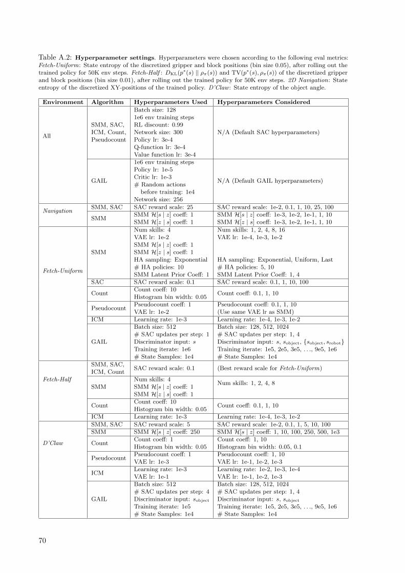
Table A.2: Hyperparameter settings. Hyperparameters were chosen according to the following eval metrics:Fetch-Uniform: State entropy of the discretized gripper and block positions (bin size 0.05), after rolling out thetrained policy for 50K env steps. Fetch-Half : DKL(p∗(s) ‖ ρπ(s)) and TV(p∗(s), ρπ(s)) of the discretized gripperand block positions (bin size 0.01), after rolling out the trained policy for 50K env steps. 2D Navigation: Stateentropy of the discretized XY-positions of the trained policy. D’Claw : State entropy of the object angle.

Environment Algorithm Hyperparameters Used Hyperparameters Considered

All

SMM, SAC,ICM, Count,Pseudocount

Batch size: 1281e6 env training stepsRL discount: 0.99Network size: 300Policy lr: 3e-4Q-function lr: 3e-4Value function lr: 3e-4

N/A (Default SAC hyperparameters)

GAIL

1e6 env training stepsPolicy lr: 1e-5Critic lr: 1e-3# Random actions

before training: 1e4Network size: 256

N/A (Default GAIL hyperparameters)

NavigationSMM, SAC SAC reward scale: 25 SAC reward scale: 1e-2, 0.1, 1, 10, 25, 100

SMMSMM H[s | z] coeff: 1SMM H[z | s] coeff: 1

SMM H[s | z] coeff: 1e-3, 1e-2, 1e-1, 1, 10SMM H[z | s] coeff: 1e-3, 1e-2, 1e-1, 1, 10

Fetch-Uniform

SMM

Num skills: 4VAE lr: 1e-2SMM H[s | z] coeff: 1SMM H[z | s] coeff: 1HA sampling: Exponential# HA policies: 10SMM Latent Prior Coeff: 1

Num skills: 1, 2, 4, 8, 16VAE lr: 1e-4, 1e-3, 1e-2

HA sampling: Exponential, Uniform, Last# HA policies: 5, 10SMM Latent Prior Coeff: 1, 4

SAC SAC reward scale: 0.1 SAC reward scale: 0.1, 1, 10, 100

CountCount coeff: 10Histogram bin width: 0.05

Count coeff: 0.1, 1, 10

PseudocountPseudocount coeff: 1VAE lr: 1e-2

Pseudocount coeff: 0.1, 1, 10(Use same VAE lr as SMM)

ICM Learning rate: 1e-3 Learning rate: 1e-4, 1e-3, 1e-2

GAIL

Batch size: 512# SAC updates per step: 1Discriminator input: sTraining iterate: 1e6# State Samples: 1e4

Batch size: 128, 512, 1024# SAC updates per step: 1, 4Discriminator input: s, sobject, {sobject, srobot}Training iterate: 1e5, 2e5, 3e5, . . ., 9e5, 1e6# State Samples: 1e4

Fetch-Half

SMM, SAC,ICM, Count

SAC reward scale: 0.1 (Best reward scale for Fetch-Uniform)

SMMNum skills: 4SMM H[s | z] coeff: 1SMM H[z | s] coeff: 1

Num skills: 1, 2, 4, 8

CountCount coeff: 10Histogram bin width: 0.05

Count coeff: 0.1, 1, 10

ICM Learning rate: 1e-3 Learning rate: 1e-4, 1e-3, 1e-2

D’Claw

SMM, SAC SAC reward scale: 5 SAC reward scale: 1e-2, 0.1, 1, 5, 10, 100SMM SMM H[s | z] coeff: 250 SMM H[s | z] coeff: 1, 10, 100, 250, 500, 1e3

CountCount coeff: 1Histogram bin width: 0.05

Count coeff: 1, 10Histogram bin width: 0.05, 0.1

PseudocountPseudocount coeff: 1VAE lr: 1e-3

Pseudocount coeff: 1, 10VAE lr: 1e-1, 1e-2, 1e-3

ICMLearning rate: 1e-3VAE lr: 1e-1

Learning rate: 1e-2, 1e-3, 1e-4VAE lr: 1e-1, 1e-2, 1e-3

GAIL

Batch size: 512# SAC updates per step: 4Discriminator input: sobjectTraining iterate: 1e5# State Samples: 1e4

Batch size: 128, 512, 1024# SAC updates per step: 1, 4Discriminator input: s, sobjectTraining iterate: 1e5, 2e5, 3e5, . . ., 9e5, 1e6# State Samples: 1e4

70

Environment M Factors (User-specified factor indices are bolded) WSC pgoal αDR

Push n = 1 256 hand x, hand y, obj x, obj y 0.2 1Push n = 2 256 hand x, hand y, obj1 x, obj1 y, obj2 x, obj2 y 0.3 1Push n = 3 512 hand x, hand y, obj1 x, obj1 y, obj2 x, obj2 y, obj3 x, obj3 y 0.4 0

PushLights n = 1 256 hand x, hand y, obj x, obj y, light 0.4 1PushLights n = 2 512 hand x, hand y, obj1 x, obj1 y, obj2 x, obj2 y, light 0.4 1PushLights n = 3 512 hand x, hand y, obj1 x, obj1 y, obj2 x, obj2 y, obj3 x, obj3 y, light 0.5 0

Pickup 512 hand y, hand z, obj y, obj z 0.4 –PickupLights 512 hand y, hand z, obj y, obj z, light 0.3 –PickupColors 512 hand y, hand z, obj y, obj z, table color, obj color 0.4 –

PickupLightsColors 512 hand y, hand z, obj y, obj z, light, table color, obj color 0.3 –Door 512 door angle 0.3 –

DoorLights 512 door angle, light 0.5 –

Table A.3: Environment-specific hyperparameters: M is the number of training images.“WSC pgoal” is the percentage of relabelled goals in WSC (Alg. 3). αDR is the VAE rewardcoefficient for SkewFit+DR in Eq. A.1.

EncoderN (z;µ(s), σ(s))

Input:48× 48× 3 image

4× 4 Conv, 32 ch, str 2Spectral normLeakyReLU

4× 4 Conv, 32 ch, str 2Spectral normLeakyReLU

4× 4 Conv, 64 ch, str 2Spectral normLeakyReLU

4× 4 Conv, 64 ch, str 2Spectral normLeakyReLU

Flatten128 Dense layerSpectral normLeakyReLU

2 ·K Dense layerOutput:

µ, σ ∈ RK

GeneratorG(z)

Input:

z ∈ RK

128 Dense layerBatch norm

ReLU3 · 3 · 64 Dense layer

Batch normReLU

Reshape 3× 3× 643× 3 Conv, 32 ch, str 2

Batch normLeakyReLU

3× 3 Conv, 16 ch, str 2Batch normLeakyReLU

6× 6 Conv, 3 ch, str 4Batch normSigmoidOutput:

48× 48× 3 image

Discriminator Body

Input:48× 48× 3 image

4× 4 Conv, 32 ch, str 2Spectral normLeakyReLU

4× 4 Conv, 32 ch, str 2Spectral normLeakyReLU

4× 4 Conv, 64 ch, str 2Spectral normLeakyReLU

4× 4 Conv, 64 ch, str 2Spectral normLeakyReLU

Flatten256 Dense layerSpectral normLeakyReLU

256 Dense layerSpectral normLeakyReLU

Output: Hidden layer h

DiscriminatorD(s1, s2, y)

Input: Weakly-labelled data(s1, s2, y) ∈ D

Output: Prediction

o1 + o2 + odiff ∈ [0, 1]

Table A.4: Disentangled representation model architecture: We slightly modified thedisentangled model architecture from Shu et al. [2019] for 48 × 48 image observations. Thediscriminator body is applied separately to s1 and s2 to compute the unconditional logits o1 ando2 respectively, and the conditional logit is computed as odiff = y · (h1 − h2), where h1, h2 are thehidden layers and y ∈ {±1}.

VAE encoder N (z;µ(s), σ(s))

Input: 48× 48× 3 image5× 5 Conv, 16 ch, str 2

ReLU3× 3 Conv, 32 ch, str 2

ReLU3× 3 Conv, 64 ch, str 2

ReLUFlatten

2 · LVAE Dense layer

Output: µ, σ ∈ RLVAE

VAE decoder

Input: z ∈ RLVAE

3 · 3 · 64 Dense layerReshape 3× 3× 64

3× 3 Conv, 32 ch, str 2ReLU

3× 3 Conv, 16 ch, str 2ReLU

Output:48× 48× 3 image

Best latent dim LVAE

Env β WSC SkewFit, RIG, HER

Push 20 256 4Pickup 30 256 16Door 20 256 16

Table A.5: VAE architecture & hyperparameters: β is the KL regularization coefficientin the β-VAE loss. We found that a smaller VAE latent dim LVAE ∈ {4, 16} worked best forSkewFit, RIG, and HER (which use the VAE for both hindsight relabelling and for the actor &critic networks), but a larger dim LVAE = 256 benefitted WSC (which only uses the VAE for theactor & critic networks).

71

Bibliography

Abbas Abdolmaleki, Jost Tobias Springenberg, Yuval Tassa, Remi Munos, Nicolas Heess, and

Martin Riedmiller. Maximum a posteriori policy optimisation. arXiv preprint arXiv:1806.06920,

2018.

Joshua Achiam, Harrison Edwards, Dario Amodei, and Pieter Abbeel. Variational option

discovery algorithms. arXiv preprint arXiv:1807.10299, 2018.

David Barber Felix Agakov. The im algorithm: a variational approach to information maximiza-

tion. Advances in Neural Information Processing Systems, 16:201, 2004.

Pulkit Agrawal, Ashvin V Nair, Pieter Abbeel, Jitendra Malik, and Sergey Levine. Learning to

poke by poking: Experiential learning of intuitive physics. In Advances in neural information

processing systems, pages 5074–5082, 2016.

Michael Ahn, Henry Zhu, Kristian Hartikainen, Hugo Ponte, Abhishek Gupta, Sergey Levine,

and Vikash Kumar. Robel: Robotics benchmarks for learning with low-cost robots. arXiv

preprint arXiv:1909.11639, 2019.

Maruan Al-Shedivat, Lisa Lee, Ruslan Salakhutdinov, and Eric Xing. On the complexity of

exploration in goal-driven navigation. arXiv preprint arXiv:1811.06889, 2018.

Peter Anderson, Qi Wu, Damien Teney, Jake Bruce, Mark Johnson, Niko Sunderhauf, Ian Reid,

Stephen Gould, and Anton van den Hengel. Vision-and-language navigation: Interpreting

visually-grounded navigation instructions in real environments. In Proceedings of the IEEE

Conference on Computer Vision and Pattern Recognition, pages 3674–3683, 2018.

Marcin Andrychowicz, Filip Wolski, Alex Ray, Jonas Schneider, Rachel Fong, Peter Welinder,

Bob McGrew, Josh Tobin, OpenAI Pieter Abbeel, and Wojciech Zaremba. Hindsight experience

replay. In Advances in Neural Information Processing Systems, pages 5048–5058, 2017.

Dzmitry Bahdanau, Felix Hill, Jan Leike, Edward Hughes, Pushmeet Kohli, and Edward

Grefenstette. Learning to follow language instructions with adversarial reward induction. arXiv

preprint arXiv:1806.01946, 2018.

73

Tadas Baltrusaitis, Chaitanya Ahuja, and Louis-Philippe Morency. Multimodal machine learning:

A survey and taxonomy. IEEE transactions on pattern analysis and machine intelligence, 41

(2):423–443, 2018.

Andre Barreto, Will Dabney, Remi Munos, Jonathan J Hunt, Tom Schaul, Hado P van Hasselt,

and David Silver. Successor features for transfer in reinforcement learning. In Advances in

neural information processing systems, pages 4055–4065, 2017.

Marc Bellemare, Sriram Srinivasan, Georg Ostrovski, Tom Schaul, David Saxton, and Remi

Munos. Unifying count-based exploration and intrinsic motivation. In Advances in Neural

Information Processing Systems, pages 1471–1479, 2016.

Emmanuel Bengio, Valentin Thomas, Joelle Pineau, Doina Precup, and Yoshua Bengio. Indepen-

dently controllable features. arXiv preprint arXiv:1703.07718, 2017.

Christopher Berner, Greg Brockman, Brooke Chan, Vicki Cheung, Przemyslaw Debiak, Christy

Dennison, David Farhi, Quirin Fischer, Shariq Hashme, Chris Hesse, et al. Dota 2 with large

scale deep reinforcement learning. arXiv preprint arXiv:1912.06680, 2019.

Daniel S Brown, Wonjoon Goo, Prabhat Nagarajan, and Scott Niekum. Extrapolating beyond

suboptimal demonstrations via inverse reinforcement learning from observations. arXiv preprint

arXiv:1904.06387, 2019.

G. Brown. Iterative solution of games by fictitious play. Activity Analysis of Production and

Allocation, 1951.

Yuri Burda, Harrison Edwards, Amos Storkey, and Oleg Klimov. Exploration by random network

distillation. arXiv preprint arXiv:1810.12894, 2018.

Devendra Singh Chaplot, Kanthashree Mysore Sathyendra, Rama Kumar Pasumarthi, Dheeraj

Rajagopal, and Ruslan Salakhutdinov. Gated-attention architectures for task-oriented language

grounding. arXiv preprint arXiv:1706.07230, 2017.

Devendra Singh Chaplot, Lisa Lee, Ruslan Salakhutdinov, Devi Parikh, and Dhruv Batra. Em-

bodied multimodal multitask learning. International Joint Conference on Artificial Intelligence

(IJCAI), 2020.

Junxiang Chen and Kayhan Batmanghelich. Weakly supervised disentanglement by pairwise

similarities. arXiv preprint arXiv:1906.01044, 2019.

Tian Qi Chen, Xuechen Li, Roger B Grosse, and David K Duvenaud. Isolating sources of

disentanglement in variational autoencoders. In Advances in Neural Information Processing

Systems, pages 2610–2620, 2018a.

Wei Chen, Heba Khamis, Ingvars Birznieks, Nathan F Lepora, and Stephen J Redmond. Tac-

tile sensors for friction estimation and incipient slip detection—toward dexterous robotic

manipulation: A review. IEEE Sensors Journal, 18(22):9049–9064, 2018b.

74

Xi Chen, Yan Duan, Rein Houthooft, John Schulman, Ilya Sutskever, and Pieter Abbeel. Infogan:

Interpretable representation learning by information maximizing generative adversarial nets.

In Advances in neural information processing systems, pages 2172–2180, 2016.

Nuttapong Chentanez, Andrew G Barto, and Satinder P Singh. Intrinsically motivated rein-

forcement learning. In Advances in neural information processing systems, pages 1281–1288,

2005.

Kyunghyun Cho, Bart Van Merrienboer, Dzmitry Bahdanau, and Yoshua Bengio. On the

properties of neural machine translation: Encoder-decoder approaches. arXiv preprint

arXiv:1409.1259, 2014.

Paul F Christiano, Jan Leike, Tom Brown, Miljan Martic, Shane Legg, and Dario Amodei. Deep

reinforcement learning from human preferences. In Advances in Neural Information Processing

Systems, pages 4299–4307, 2017.

John D Co-Reyes, YuXuan Liu, Abhishek Gupta, Benjamin Eysenbach, Pieter Abbeel, and

Sergey Levine. Self-consistent trajectory autoencoder: Hierarchical reinforcement learning

with trajectory embeddings. arXiv preprint arXiv:1806.02813, 2018.

Cedric Colas, Olivier Sigaud, and Pierre-Yves Oudeyer. Curious: Intrinsically motivated multi-

task, multi-goal reinforcement learning. arXiv preprint arXiv:1810.06284, 2018.

Ravinder S Dahiya, Giorgio Metta, Maurizio Valle, and Giulio Sandini. Tactile sensing—from

humans to humanoids. IEEE transactions on robotics, 26(1):1–20, 2009.

Abhishek Das, Samyak Datta, Georgia Gkioxari, Stefan Lee, Devi Parikh, and Dhruv Batra.

Embodied question answering. arXiv preprint arXiv:1711.11543, 2017.

Abhishek Das, Samyak Datta, Georgia Gkioxari, Stefan Lee, Devi Parikh, and Dhruv Batra.

Embodied question answering. In Proceedings of the IEEE Conference on Computer Vision

and Pattern Recognition, pages 1–10, 2018.

Sudeep Dasari, Frederik Ebert, Stephen Tian, Suraj Nair, Bernadette Bucher, Karl Schmeckpeper,

Siddharth Singh, Sergey Levine, and Chelsea Finn. Robonet: Large-scale multi-robot learning.

arXiv preprint arXiv:1910.11215, 2019.

Constantinos Daskalakis and Qinxuan Pan. A counter-example to karlin’s strong conjecture for

fictitious play. In 2014 IEEE 55th Annual Symposium on Foundations of Computer Science,

pages 11–20. IEEE, 2014.

Victoria Dean, Shubham Tulsiani, and Abhinav Gupta. See, hear, explore: Curiosity via

audio-visual association. arXiv preprint arXiv:2007.03669, 2020.

Joseph DelPreto, Jeffrey I Lipton, Lindsay Sanneman, Aidan J Fay, Christopher Fourie,

Changhyun Choi, and Daniela Rus. Helping robots learn: a human-robot master-apprentice

model using demonstrations via virtual reality teleoperation. In 2020 IEEE International

Conference on Robotics and Automation (ICRA), pages 10226–10233. IEEE, 2020.

75

Nat Dilokthanakul, Christos Kaplanis, Nick Pawlowski, and Murray Shanahan. Feature control

as intrinsic motivation for hierarchical reinforcement learning. IEEE transactions on neural

networks and learning systems, 30(11):3409–3418, 2019.

Alexey Dosovitskiy and Vladlen Koltun. Learning to act by predicting the future. arXiv preprint

arXiv:1611.01779, 2016.

Yan Duan, John Schulman, Xi Chen, Peter L Bartlett, Ilya Sutskever, and Pieter Abbeel. Rl2:

Fast reinforcement learning via slow reinforcement learning. arXiv preprint arXiv:1611.02779,

2016.

Yan Duan, Marcin Andrychowicz, Bradly Stadie, OpenAI Jonathan Ho, Jonas Schneider, Ilya

Sutskever, Pieter Abbeel, and Wojciech Zaremba. One-shot imitation learning. In Advances in

neural information processing systems, pages 1087–1098, 2017.

Babak Esmaeili, Hao Wu, Sarthak Jain, Alican Bozkurt, Narayanaswamy Siddharth, Brooks

Paige, Dana H Brooks, Jennifer Dy, and Jan-Willem van de Meent. Structured disentangled

representations. arXiv preprint arXiv:1804.02086, 2018.

Benjamin Eysenbach, Abhishek Gupta, Julian Ibarz, and Sergey Levine. Diversity is all you

need: Learning skills without a reward function. arXiv preprint arXiv:1802.06070, 2018.

Taylor A Kessler Faulkner, Elaine Schaertl Short, and Andrea L Thomaz. Interactive reinforcement

learning with inaccurate feedback. In 2020 IEEE International Conference on Robotics and

Automation (ICRA), pages 7498–7504. IEEE, 2020.

Chelsea Finn and Sergey Levine. Deep visual foresight for planning robot motion. In 2017 IEEE

International Conference on Robotics and Automation (ICRA), pages 2786–2793. IEEE, 2017.

Chelsea Finn, Sergey Levine, and Pieter Abbeel. Guided cost learning: Deep inverse optimal

control via policy optimization. In International Conference on Machine Learning, pages

49–58, 2016a.

Chelsea Finn, Xin Yu Tan, Yan Duan, Trevor Darrell, Sergey Levine, and Pieter Abbeel. Deep

spatial autoencoders for visuomotor learning. In 2016 IEEE International Conference on

Robotics and Automation (ICRA), pages 512–519. IEEE, 2016b.

Chelsea Finn, Pieter Abbeel, and Sergey Levine. Model-agnostic meta-learning for fast adaptation

of deep networks. In Proceedings of the 34th International Conference on Machine Learning-

Volume 70, pages 1126–1135. JMLR. org, 2017.

Maxwell Forbes, Rajesh PN Rao, Luke Zettlemoyer, and Maya Cakmak. Robot programming

by demonstration with situated spatial language understanding. In 2015 IEEE International

Conference on Robotics and Automation (ICRA), pages 2014–2020. IEEE, 2015.

Meire Fortunato, Mohammad Gheshlaghi Azar, Bilal Piot, Jacob Menick, Ian Osband, Alex

Graves, Vlad Mnih, Remi Munos, Demis Hassabis, Olivier Pietquin, et al. Noisy networks for

exploration. arXiv preprint arXiv:1706.10295, 2017.

76

Justin Fu, Katie Luo, and Sergey Levine. Learning robust rewards with adversarial inverse

reinforcement learning. arXiv preprint arXiv:1710.11248, 2017.

Justin Fu, Katie Luo, and Sergey Levine. Learning robust rewards with adverserial inverse

reinforcement learning. In International Conference on Learning Representations, 2018a. URL

https://openreview.net/forum?id=rkHywl-A-.

Justin Fu, Avi Singh, Dibya Ghosh, Larry Yang, and Sergey Levine. Variational inverse control

with events: A general framework for data-driven reward definition. In Advances in Neural

Information Processing Systems, pages 8538–8547, 2018b.

Justin Fu, Anoop Korattikara, Sergey Levine, and Sergio Guadarrama. From language to

goals: Inverse reinforcement learning for vision-based instruction following. arXiv preprint

arXiv:1902.07742, 2019.

Akira Fukui, Dong Huk Park, Daylen Yang, Anna Rohrbach, Trevor Darrell, and Marcus

Rohrbach. Multimodal compact bilinear pooling for visual question answering and visual

grounding. arXiv preprint arXiv:1606.01847, 2016.

Aviv Gabbay and Yedid Hoshen. Latent optimization for non-adversarial representation disen-

tanglement. arXiv preprint arXiv:1906.11796, 2019.

Carles Gelada, Saurabh Kumar, Jacob Buckman, Ofir Nachum, and Marc G Bellemare. Deep-

mdp: Learning continuous latent space models for representation learning. arXiv preprint

arXiv:1906.02736, 2019.

Seyed Kamyar Seyed Ghasemipour, Richard Zemel, and Shixiang Gu. A divergence minimization

perspective on imitation learning methods. Conference on Robot Learning (CoRL), 2019.

Leilani H Gilpin, David Bau, Ben Z Yuan, Ayesha Bajwa, Michael Specter, and Lalana Kagal.

Explaining explanations: An overview of interpretability of machine learning. In 2018 IEEE

5th International Conference on data science and advanced analytics (DSAA), pages 80–89.

IEEE, 2018.

Xavier Glorot, Antoine Bordes, and Yoshua Bengio. Deep sparse rectifier neural networks. In

Proceedings of the fourteenth international conference on artificial intelligence and statistics,

pages 315–323, 2011.

Daniel Gordon, Aniruddha Kembhavi, Mohammad Rastegari, Joseph Redmon, Dieter Fox, and

Ali Farhadi. Iqa: Visual question answering in interactive environments. In Proceedings of the

IEEE Conference on Computer Vision and Pattern Recognition, pages 4089–4098, 2018.

Anirudh Goyal, Riashat Islam, Daniel Strouse, Zafarali Ahmed, Matthew Botvinick, Hugo

Larochelle, Sergey Levine, and Yoshua Bengio. Infobot: Transfer and exploration via the

information bottleneck. arXiv preprint arXiv:1901.10902, 2019.

Shixiang Gu, Ethan Holly, Timothy Lillicrap, and Sergey Levine. Deep reinforcement learning

for robotic manipulation with asynchronous off-policy updates. In 2017 IEEE international

conference on robotics and automation (ICRA), pages 3389–3396. IEEE, 2017.

77

Florent Guenter, Micha Hersch, Sylvain Calinon, and Aude Billard. Reinforcement learning for

imitating constrained reaching movements. Advanced Robotics, 21(13):1521–1544, 2007.

Abhishek Gupta, Russell Mendonca, YuXuan Liu, Pieter Abbeel, and Sergey Levine. Meta-

reinforcement learning of structured exploration strategies. In Advances in Neural Information

Processing Systems, pages 5302–5311, 2018.

Saurabh Gupta, James Davidson, Sergey Levine, Rahul Sukthankar, and Jitendra Malik. Cognitive

mapping and planning for visual navigation. arXiv preprint arXiv:1702.03920, 3, 2017a.

Tanmay Gupta, Kevin J Shih, Saurabh Singh, Derek Hoiem, Kevin J Shih, Arun Mallya, Wei Di,

Vignesh Jagadeesh, Robinson Piramuthu, K Shih, et al. Aligned image-word representations

improve inductive transfer across vision-language tasks. In ICCV, pages 4223–4232, 2017b.

Tuomas Haarnoja, Aurick Zhou, Pieter Abbeel, and Sergey Levine. Soft actor-critic: Off-

policy maximum entropy deep reinforcement learning with a stochastic actor. arXiv preprint

arXiv:1801.01290, 2018.

Dylan Hadfield-Menell, Smitha Milli, Pieter Abbeel, Stuart J Russell, and Anca Dragan. Inverse

reward design. In Advances in neural information processing systems, pages 6765–6774, 2017.

Danijar Hafner, Timothy Lillicrap, Ian Fischer, Ruben Villegas, David Ha, Honglak Lee,

and James Davidson. Learning latent dynamics for planning from pixels. arXiv preprint

arXiv:1811.04551, 2018.

Karol Hausman, Jost Tobias Springenberg, Ziyu Wang, Nicolas Heess, and Martin Riedmiller.

Learning an embedding space for transferable robot skills. 2018.

Elad Hazan, Sham M Kakade, Karan Singh, and Abby Van Soest. Provably efficient maximum

entropy exploration. arXiv preprint arXiv:1812.02690, 2018.

David Held, Xinyang Geng, Carlos Florensa, and Pieter Abbeel. Automatic goal generation for

reinforcement learning agents. arXiv preprint arXiv:1705.06366, 2017.

Karl Moritz Hermann, Felix Hill, Simon Green, Fumin Wang, Ryan Faulkner, Hubert Soyer,

David Szepesvari, Wojtek Czarnecki, Max Jaderberg, Denis Teplyashin, et al. Grounded

language learning in a simulated 3d world. arXiv preprint arXiv:1706.06551, 2017.

Irina Higgins, Loic Matthey, Arka Pal, Christopher Burgess, Xavier Glorot, Matthew Botvinick,

Shakir Mohamed, and Alexander Lerchner. beta-vae: Learning basic visual concepts with a

constrained variational framework. Iclr, 2(5):6, 2017.

Irina Higgins, David Amos, David Pfau, Sebastien Racaniere, Loic Matthey, Danilo Rezende,

and Alexander Lerchner. Towards a definition of disentangled representations. arXiv preprint

arXiv:1812.02230, 2018.

Jonathan Ho and Stefano Ermon. Generative adversarial imitation learning. In Advances in

Neural Information Processing Systems, pages 4565–4573, 2016.

78

Roger A Horn. The hadamard product. In Proc. Symp. Appl. Math, volume 40, pages 87–169,

1990.

Rein Houthooft, Xi Chen, Yan Duan, John Schulman, Filip De Turck, and Pieter Abbeel. Vime:

Variational information maximizing exploration. In Advances in Neural Information Processing

Systems, pages 1109–1117, 2016.

Robert D Howe. Tactile sensing and control of robotic manipulation. Advanced Robotics, 8(3):

245–261, 1993.

Drew A Hudson and Christopher D Manning. Compositional attention networks for machine

reasoning. arXiv preprint arXiv:1803.03067, 2018.

Max Jaderberg, Volodymyr Mnih, Wojciech Marian Czarnecki, Tom Schaul, Joel Z Leibo, David

Silver, and Koray Kavukcuoglu. Reinforcement learning with unsupervised auxiliary tasks.

arXiv preprint arXiv:1611.05397, 2016.

Yiding Jiang, Shixiang Gu, Kevin Murphy, and Chelsea Finn. Language as an abstraction for

hierarchical deep reinforcement learning. arXiv preprint arXiv:1906.07343, 2019.

Yohan Jo, Lisa Lee, and Shruti Palaskar. Combining lstm and latent topic modeling for mortality

prediction. arXiv preprint arXiv:1709.02842, 2017.

Leslie Pack Kaelbling. Learning to achieve goals. In IJCAI, pages 1094–1099. Citeseer, 1993.

Lukasz Kaiser, Mohammad Babaeizadeh, Piotr Milos, Blazej Osinski, Roy H Campbell, Konrad

Czechowski, Dumitru Erhan, Chelsea Finn, Piotr Kozakowski, Sergey Levine, et al. Model-

based reinforcement learning for atari. arXiv preprint arXiv:1903.00374, 2019.

Hilbert J Kappen, Vicenc Gomez, and Manfred Opper. Optimal control as a graphical model

inference problem. Machine learning, 87(2):159–182, 2012.

Micha l Kempka, Marek Wydmuch, Grzegorz Runc, Jakub Toczek, and Wojciech Jaskowski.

ViZDoom: A Doom-based AI research platform for visual reinforcement learning. In IEEE

Conference on Computational Intelligence and Games, pages 341–348. IEEE, Sep 2016.

Hyunjik Kim and Andriy Mnih. Disentangling by factorising. arXiv preprint arXiv:1802.05983,

2018.

W Bradley Knox and Peter Stone. Interactively shaping agents via human reinforcement: The

tamer framework. In Proceedings of the fifth international conference on Knowledge capture,

pages 9–16, 2009.

Jens Kober, Betty Mohler, and Jan Peters. Imitation and reinforcement learning for motor

primitives with perceptual coupling. In From motor learning to interaction learning in robots,

pages 209–225. Springer, 2010.

J Zico Kolter and Andrew Y Ng. Near-bayesian exploration in polynomial time. In Proceedings

of the 26th annual international conference on machine learning, pages 513–520, 2009.

79

Brenden M Lake, Tomer D Ullman, Joshua B Tenenbaum, and Samuel J Gershman. Building

machines that learn and think like people. Behavioral and brain sciences, 40, 2017.

Guillaume Lample and Devendra Singh Chaplot. Playing FPS games with deep reinforcement

learning. In Thirty-First AAAI Conference on Artificial Intelligence, 2017.

Michael Laskey, Jonathan Lee, Roy Fox, Anca Dragan, and Ken Goldberg. Dart: Noise injection

for robust imitation learning. arXiv preprint arXiv:1703.09327, 2017.

Yann LeCun, Yoshua Bengio, et al. Convolutional networks for images, speech, and time series.

The handbook of brain theory and neural networks, 3361(10):1995, 1995.

Alex X Lee, Anusha Nagabandi, Pieter Abbeel, and Sergey Levine. Stochastic latent actor-critic:

Deep reinforcement learning with a latent variable model. arXiv preprint arXiv:1907.00953,

2019a.

Dongheui Lee and Christian Ott. Incremental kinesthetic teaching of motion primitives using

the motion refinement tube. Autonomous Robots, 31(2):115–131, 2011.

Kimin Lee, Laura Smith, and Pieter Abbeel. Pebble: Feedback-efficient interactive rein-

forcement learning via relabeling experience and unsupervised pre-training. arXiv preprint

arXiv:2106.05091, 2021.

Lisa Lee, Emilio Parisotto, Devendra Singh Chaplot, Eric Xing, and Ruslan Salakhutdinov.

Gated path planning networks. In International Conference on Machine Learning (ICML),

pages 2947–2955. PMLR, 2018.

Lisa Lee, Benjamin Eysenbach, Emilio Parisotto, Eric Xing, Sergey Levine, and Ruslan Salakhut-

dinov. Efficient exploration via state marginal matching. arXiv preprint arXiv:1906.05274,

2019b.

Lisa Lee, Benjamin Eysenbach, Ruslan Salakhutdinov, Chelsea Finn, et al. Weakly-supervised

reinforcement learning for controllable behavior. Neural Information Processing Systems

(NeurIPS), 2020.

Sergey Levine. Reinforcement learning and control as probabilistic inference: Tutorial and review.

arXiv preprint arXiv:1805.00909, 2018.

Guangliang Li, Randy Gomez, Keisuke Nakamura, Jinying Lin, Qilei Zhang, and Bo He. Im-

proving interactive reinforcement agent planning with human demonstration. arXiv preprint

arXiv:1904.08621, 2019.

Xiaodan Liang, Lisa Lee, Wei Dai, and Eric P Xing. Dual motion gan for future-flow embedded

video prediction. In Proceedings of the IEEE International Conference on Computer Vision

(ICCV), pages 1744–1752, 2017a.

Xiaodan Liang, Lisa Lee, and Eric P Xing. Deep variation-structured reinforcement learning

for visual relationship and attribute detection. In Proceedings of the IEEE conference on

Computer Vision and Pattern Recognition (CVPR), pages 848–857, 2017b.

80

Timothy P Lillicrap, Jonathan J Hunt, Alexander Pritzel, Nicolas Heess, Tom Erez, Yuval Tassa,

David Silver, and Daan Wierstra. Continuous control with deep reinforcement learning. arXiv

preprint arXiv:1509.02971, 2015.

Guan-Horng Liu, Avinash Siravuru, Sai Prabhakar, Manuela Veloso, and George Kantor. Learning

end-to-end multimodal sensor policies for autonomous navigation. In Conference on Robot

Learning, pages 249–261. PMLR, 2017.

Francesco Locatello, Stefan Bauer, Mario Lucic, Gunnar Ratsch, Sylvain Gelly, Bernhard

Scholkopf, and Olivier Bachem. Challenging common assumptions in the unsupervised learning

of disentangled representations. arXiv preprint arXiv:1811.12359, 2018.

James MacGlashan, Monica Babes-Vroman, Marie desJardins, Michael L Littman, Smaranda

Muresan, Shawn Squire, Stefanie Tellex, Dilip Arumugam, and Lei Yang. Grounding english

commands to reward functions. In Robotics: Science and Systems, 2015.

Marios C Machado, Marc G Bellemare, and Michael Bowling. A laplacian framework for option

discovery in reinforcement learning. In Proceedings of the 34th International Conference on

Machine Learning-Volume 70, pages 2295–2304. JMLR. org, 2017.

Sridhar Mahadevan. Proto-value functions: Developmental reinforcement learning. In Proceedings

of the 22nd international conference on Machine learning, pages 553–560. ACM, 2005.

Ajay Mandlekar, Yuke Zhu, Animesh Garg, Jonathan Booher, Max Spero, Albert Tung, Julian

Gao, John Emmons, Anchit Gupta, Emre Orbay, et al. Roboturk: A crowdsourcing platform

for robotic skill learning through imitation. arXiv preprint arXiv:1811.02790, 2018.

Ajay Mandlekar, Danfei Xu, Roberto Martın-Martın, Yuke Zhu, Li Fei-Fei, and Silvio

Savarese. Human-in-the-loop imitation learning using remote teleoperation. arXiv preprint

arXiv:2012.06733, 2020.

Loic Matthey, Irina Higgins, Demis Hassabis, and Alexander Lerchner. dsprites: Disentanglement

testing sprites dataset. https://github.com/deepmind/dsprites-dataset/, 2017.

Hongyuan Mei, Mohit Bansal, and Matthew R Walter. Listen, attend, and walk: Neural mapping

of navigational instructions to action sequences. In Thirtieth AAAI Conference on Artificial

Intelligence, 2016.

Josh Merel, Leonard Hasenclever, Alexandre Galashov, Arun Ahuja, Vu Pham, Greg Wayne,

Yee Whye Teh, and Nicolas Heess. Neural probabilistic motor primitives for humanoid control.

arXiv preprint arXiv:1811.11711, 2018.

Piotr Mirowski, Razvan Pascanu, Fabio Viola, Hubert Soyer, Andrew J Ballard, Andrea Banino,

Misha Denil, Ross Goroshin, Laurent Sifre, Koray Kavukcuoglu, et al. Learning to navigate in

complex environments. arXiv preprint arXiv:1611.03673, 2016.

Nikhil Mishra, Mostafa Rohaninejad, Xi Chen, and Pieter Abbeel. A simple neural attentive

meta-learner. arXiv preprint arXiv:1707.03141, 2017.

81

Dipendra K Misra, Jaeyong Sung, Kevin Lee, and Ashutosh Saxena. Tell me dave: Context-

sensitive grounding of natural language to manipulation instructions. The International Journal

of Robotics Research, 35(1-3):281–300, 2016.

Dipendra K Misra, John Langford, and Yoav Artzi. Mapping instructions and visual observations

to actions with reinforcement learning. arXiv preprint arXiv:1704.08795, 2017.

Volodymyr Mnih, Koray Kavukcuoglu, David Silver, Alex Graves, Ioannis Antonoglou, Daan

Wierstra, and Martin Riedmiller. Playing atari with deep reinforcement learning. arXiv

preprint arXiv:1312.5602, 2013.

Volodymyr Mnih, Adria Puigdomenech Badia, Mehdi Mirza, Alex Graves, Timothy P Lilli-

crap, Tim Harley, David Silver, and Koray Kavukcuoglu. Asynchronous methods for deep

reinforcement learning. In ICML, 2016.

Katharina Mulling, Jens Kober, Oliver Kroemer, and Jan Peters. Learning to select and generalize

striking movements in robot table tennis. The International Journal of Robotics Research, 32

(3):263–279, 2013.

Ofir Nachum, Shixiang Gu, Honglak Lee, and Sergey Levine. Near-optimal representation

learning for hierarchical reinforcement learning. arXiv preprint arXiv:1810.01257, 2018.

Ashvin V Nair, Vitchyr Pong, Murtaza Dalal, Shikhar Bahl, Steven Lin, and Sergey Levine. Visual

reinforcement learning with imagined goals. In Advances in Neural Information Processing

Systems, pages 9191–9200, 2018.

John Nash. Non-cooperative games. Annals of mathematics, pages 286–295, 1951.

Tianwei Ni, Harshit Sikchi, Yufei Wang, Tejus Gupta, Lisa Lee, and Benjamin Eysenbach. F-irl:

Inverse reinforcement learning via state marginal matching. Conference on Robot Learning

(CoRL), 2020.

Junhyuk Oh, Satinder Singh, Honglak Lee, and Pushmeet Kohli. Zero-shot task generalization

with multi-task deep reinforcement learning. arXiv preprint arXiv:1706.05064, 2017.

Pierre-Yves Oudeyer, Frdric Kaplan, and Verena V Hafner. Intrinsic motivation systems for

autonomous mental development. IEEE transactions on evolutionary computation, 11(2):

265–286, 2007.

Deepak Pathak, Pulkit Agrawal, Alexei A Efros, and Trevor Darrell. Curiosity-driven exploration

by self-supervised prediction. In Proceedings of the IEEE Conference on Computer Vision and

Pattern Recognition Workshops, pages 16–17, 2017.

Deepak Pathak, Parsa Mahmoudieh, Guanghao Luo, Pulkit Agrawal, Dian Chen, Yide Shentu,

Evan Shelhamer, Jitendra Malik, Alexei A Efros, and Trevor Darrell. Zero-shot visual imitation.

In Proceedings of the IEEE Conference on Computer Vision and Pattern Recognition Workshops,

pages 2050–2053, 2018.

82

Xue Bin Peng, Angjoo Kanazawa, Jitendra Malik, Pieter Abbeel, and Sergey Levine. Sfv:

Reinforcement learning of physical skills from videos. ACM Transactions On Graphics (TOG),

37(6):1–14, 2018.

Ethan Perez, Florian Strub, Harm De Vries, Vincent Dumoulin, and Aaron Courville. Film:

Visual reasoning with a general conditioning layer. arXiv preprint arXiv:1709.07871, 2017.

Jan Peters, Katharina Mulling, and Yasemin Altun. Relative entropy policy search. In Twenty-

Fourth AAAI Conference on Artificial Intelligence, 2010.

Matthias Plappert, Rein Houthooft, Prafulla Dhariwal, Szymon Sidor, Richard Y Chen, Xi Chen,

Tamim Asfour, Pieter Abbeel, and Marcin Andrychowicz. Parameter space noise for exploration.

arXiv preprint arXiv:1706.01905, 2017.

Matthias Plappert, Marcin Andrychowicz, Alex Ray, Bob McGrew, Bowen Baker, Glenn Powell,

Jonas Schneider, Josh Tobin, Maciek Chociej, Peter Welinder, et al. Multi-goal reinforce-

ment learning: Challenging robotics environments and request for research. arXiv preprint

arXiv:1802.09464, 2018.

Vitchyr Pong, Shixiang Gu, Murtaza Dalal, and Sergey Levine. Temporal difference models:

Model-free deep rl for model-based control. arXiv preprint arXiv:1802.09081, 2018.

Vitchyr H Pong, Murtaza Dalal, Steven Lin, Ashvin Nair, Shikhar Bahl, and Sergey Levine. Skew-

fit: State-covering self-supervised reinforcement learning. arXiv preprint arXiv:1903.03698,

2019.

Justin K Pugh, Lisa B Soros, and Kenneth O Stanley. Quality diversity: A new frontier for

evolutionary computation. Frontiers in Robotics and AI, 3:40, 2016.

Martin L Puterman. Markov Decision Processes.: Discrete Stochastic Dynamic Programming.

John Wiley & Sons, 2014.

Kate Rakelly, Aurick Zhou, Deirdre Quillen, Chelsea Finn, and Sergey Levine. Efficient

off-policy meta-reinforcement learning via probabilistic context variables. arXiv preprint

arXiv:1903.08254, 2019.

Nathan D Ratliff, J Andrew Bagnell, and Martin A Zinkevich. Maximum margin planning. In

Proceedings of the 23rd international conference on Machine learning, pages 729–736, 2006.

Konrad Rawlik, Marc Toussaint, and Sethu Vijayakumar. On stochastic optimal control and rein-

forcement learning by approximate inference. In Twenty-Third International Joint Conference

on Artificial Intelligence, 2013.

Julia Robinson. An iterative method of solving a game. Annals of mathematics, pages 296–301,

1951.

Manolis Savva, Angel X. Chang, Alexey Dosovitskiy, Thomas Funkhouser, and Vladlen

Koltun. MINOS: Multimodal indoor simulator for navigation in complex environments.

arXiv:1712.03931, 2017.

83

Tom Schaul, Daniel Horgan, Karol Gregor, and David Silver. Universal value function approxi-

mators. In International conference on machine learning, pages 1312–1320, 2015.

Jurgen Schmidhuber. A possibility for implementing curiosity and boredom in model-building

neural controllers. In Proc. of the international conference on simulation of adaptive behavior:

From animals to animats, pages 222–227, 1991.

Jurgen Schmidhuber. Formal theory of creativity, fun, and intrinsic motivation (1990–2010).

IEEE Transactions on Autonomous Mental Development, 2(3):230–247, 2010.

John Schulman, Sergey Levine, Pieter Abbeel, Michael Jordan, and Philipp Moritz. Trust region

policy optimization. In International conference on machine learning, pages 1889–1897, 2015.

John Schulman, Filip Wolski, Prafulla Dhariwal, Alec Radford, and Oleg Klimov. Proximal

policy optimization algorithms. arXiv preprint arXiv:1707.06347, 2017.

Evan Shelhamer, Parsa Mahmoudieh, Max Argus, and Trevor Darrell. Loss is its own reward:

Self-supervision for reinforcement learning. arXiv preprint arXiv:1612.07307, 2016.

Rui Shu, Yining Chen, Abhishek Kumar, Stefano Ermon, and Ben Poole. Weakly supervised

disentanglement with guarantees. arXiv preprint arXiv:1910.09772, 2019.

David Silver, Aja Huang, Chris J Maddison, Arthur Guez, Laurent Sifre, George Van Den Driess-

che, Julian Schrittwieser, Ioannis Antonoglou, Veda Panneershelvam, Marc Lanctot, et al.

Mastering the game of go with deep neural networks and tree search. Nature, 529(7587):

484–489, 2016.

David Silver, Thomas Hubert, Julian Schrittwieser, Ioannis Antonoglou, Matthew Lai, Arthur

Guez, Marc Lanctot, Laurent Sifre, Dharshan Kumaran, Thore Graepel, et al. Mastering

chess and shogi by self-play with a general reinforcement learning algorithm. arXiv preprint

arXiv:1712.01815, 2017.

Avi Singh, Larry Yang, Kristian Hartikainen, Chelsea Finn, and Sergey Levine. End-to-end

robotic reinforcement learning without reward engineering. arXiv preprint arXiv:1904.07854,

2019.

Hailuo Song, Ao Li, Tong Wang, and Minghui Wang. Multimodal deep reinforcement learning

with auxiliary task for obstacle avoidance of indoor mobile robot. Sensors, 21(4):1363, 2021.

Thomas H Speeter. A tactile sensing system for robotic manipulation. The International Journal

of Robotics Research, 9(6):25–36, 1990.

Bradly C Stadie, Sergey Levine, and Pieter Abbeel. Incentivizing exploration in reinforcement

learning with deep predictive models. arXiv preprint arXiv:1507.00814, 2015.

Kenneth O Stanley and Risto Miikkulainen. Evolving neural networks through augmenting

topologies. Evolutionary computation, 10(2):99–127, 2002.

84

Adrien Ali Taıga, William Fedus, Marlos C Machado, Aaron Courville, and Marc G Bellemare.

Benchmarking bonus-based exploration methods on the arcade learning environment. arXiv

preprint arXiv:1908.02388, 2019.

Haoran Tang, Rein Houthooft, Davis Foote, Adam Stooke, OpenAI Xi Chen, Yan Duan, John

Schulman, Filip DeTurck, and Pieter Abbeel. # exploration: A study of count-based exploration

for deep reinforcement learning. In Advances in neural information processing systems, pages

2753–2762, 2017.

Stefanie A Tellex, Thomas Fleming Kollar, Steven R Dickerson, Matthew R Walter, Ashis

Banerjee, Seth Teller, and Nicholas Roy. Understanding natural language commands for

robotic navigation and mobile manipulation. 2011.

Evangelos A Theodorou and Emanuel Todorov. Relative entropy and free energy dualities:

Connections to path integral and kl control. In 2012 IEEE 51st IEEE Conference on Decision

and Control (CDC), pages 1466–1473. IEEE, 2012.

Valentin Thomas, Jules Pondard, Emmanuel Bengio, Marc Sarfati, Philippe Beaudoin, Marie-

Jean Meurs, Joelle Pineau, Doina Precup, and Yoshua Bengio. Independently controllable

features. arXiv preprint arXiv:1708.01289, 2017.

Marc Toussaint and Amos Storkey. Probabilistic inference for solving discrete and continuous

state markov decision processes. In Proceedings of the 23rd international conference on Machine

learning, pages 945–952. ACM, 2006.

Hsiao-Yu Tung, Adam W Harley, Liang-Kang Huang, and Katerina Fragkiadaki. Reward learning

from narrated demonstrations. In Proceedings of the IEEE Conference on Computer Vision

and Pattern Recognition, pages 7004–7013, 2018.

Sjoerd van Steenkiste, Francesco Locatello, Jurgen Schmidhuber, and Olivier Bachem. Are

disentangled representations helpful for abstract visual reasoning? In Advances in Neural

Information Processing Systems, pages 14222–14235, 2019.

Mel Vecerik, Oleg Sushkov, David Barker, Thomas Rothorl, Todd Hester, and Jon Scholz. A

practical approach to insertion with variable socket position using deep reinforcement learning.

In 2019 International Conference on Robotics and Automation (ICRA), pages 754–760. IEEE,

2019.

Oriol Vinyals, Igor Babuschkin, Wojciech M Czarnecki, Michael Mathieu, Andrew Dudzik, Juny-

oung Chung, David H Choi, Richard Powell, Timo Ewalds, Petko Georgiev, et al. Grandmaster

level in starcraft ii using multi-agent reinforcement learning. Nature, 575(7782):350–354, 2019.

Manuel Watter, Jost Springenberg, Joschka Boedecker, and Martin Riedmiller. Embed to control:

A locally linear latent dynamics model for control from raw images. In Advances in neural

information processing systems, pages 2746–2754, 2015.

Yi Wu, Yuxin Wu, Georgia Gkioxari, and Yuandong Tian. Building generalizable agents with a

realistic and rich 3d environment. arXiv preprint arXiv:1801.02209, 2018.

85

Annie Xie, Avi Singh, Sergey Levine, and Chelsea Finn. Few-shot goal inference for visuomotor

learning and planning. arXiv preprint arXiv:1810.00482, 2018.

Dan Xie, Sinisa Todorovic, and Song-Chun Zhu. Inferring ”dark matter” and ”dark energy” from

videos. In The IEEE International Conference on Computer Vision (ICCV), December 2013.

Huijuan Xu and Kate Saenko. Ask, attend and answer: Exploring question-guided spatial

attention for visual question answering. In European Conference on Computer Vision, pages

451–466. Springer, 2016.

Tianbing Xu, Qiang Liu, Liang Zhao, and Jian Peng. Learning to explore with meta-policy

gradient. arXiv preprint arXiv:1803.05044, 2018.

Fusun Yaman, Thomas J Walsh, Michael L Littman, et al. Learning lexicographic preference

models. In Preference learning, pages 251–272. Springer, 2010.

Denis Yarats, Amy Zhang, Ilya Kostrikov, Brandon Amos, Joelle Pineau, and Rob Fergus.

Improving sample efficiency in model-free reinforcement learning from images. arXiv preprint

arXiv:1910.01741, 2019.

Haonan Yu, Xiaochen Lian, Haichao Zhang, and Wei Xu. Guided feature transformation (gft):

A neural language grounding module for embodied agents. arXiv preprint arXiv:1805.08329,

2018a.

Haonan Yu, Haichao Zhang, and Wei Xu. Interactive grounded language acquisition and

generalization in a 2d world. arXiv preprint arXiv:1802.01433, 2018b.

Tianhe Yu, Gleb Shevchuk, Dorsa Sadigh, and Chelsea Finn. Unsupervised visuomotor control

through distributional planning networks. arXiv preprint arXiv:1902.05542, 2019.

Marvin Zhang, Sharad Vikram, Laura Smith, Pieter Abbeel, Matthew J Johnson, and Sergey

Levine. Solar: Deep structured latent representations for model-based reinforcement learning.

arXiv preprint arXiv:1808.09105, 2018a.

Tianhao Zhang, Zoe McCarthy, Owen Jow, Dennis Lee, Xi Chen, Ken Goldberg, and Pieter Abbeel.

Deep imitation learning for complex manipulation tasks from virtual reality teleoperation. In

2018 IEEE International Conference on Robotics and Automation (ICRA), pages 5628–5635.

IEEE, 2018b.

Hang Zhao, Chuang Gan, Andrew Rouditchenko, Carl Vondrick, Josh McDermott, and Antonio

Torralba. The sound of pixels. arXiv preprint arXiv:1804.03160, 2018.

Henry Zhu, Abhishek Gupta, Aravind Rajeswaran, Sergey Levine, and Vikash Kumar. Dexterous

manipulation with deep reinforcement learning: Efficient, general, and low-cost. In 2019

International Conference on Robotics and Automation (ICRA), pages 3651–3657. IEEE, 2019.

Yuke Zhu, Roozbeh Mottaghi, Eric Kolve, Joseph J Lim, Abhinav Gupta, Li Fei-Fei, and Ali

Farhadi. Target-driven visual navigation in indoor scenes using deep reinforcement learning. In

Robotics and Automation (ICRA), 2017 IEEE International Conference on, pages 3357–3364.

IEEE, 2017.

86

Brian D Ziebart. Modeling purposeful adaptive behavior with the principle of maximum causal

entropy. 2010.

Brian D Ziebart, Andrew L Maas, J Andrew Bagnell, and Anind K Dey. Maximum entropy

inverse reinforcement learning. In Aaai, volume 8, pages 1433–1438. Chicago, IL, USA, 2008.

Brian D Ziebart, Nathan Ratliff, Garratt Gallagher, Christoph Mertz, Kevin Peterson, J Andrew

Bagnell, Martial Hebert, Anind K Dey, and Siddhartha Srinivasa. Planning-based prediction for

pedestrians. In 2009 IEEE/RSJ International Conference on Intelligent Robots and Systems,

pages 3931–3936. IEEE, 2009.

87