learning feature representations for music...
TRANSCRIPT

LEARNING FEATURE REPRESENTATIONS FOR MUSIC
CLASSIFICATION
A DISSERTATION
SUBMITTED TO THE DEPARTMENT OF MUSIC
AND THE COMMITTEE ON GRADUATE STUDIES
OF STANFORD UNIVERSITY
IN PARTIAL FULFILLMENT OF THE REQUIREMENTS
FOR THE DEGREE OF
DOCTOR OF PHILOSOPHY
Juhan Nam
December 2012

http://creativecommons.org/licenses/by-nc/3.0/us/
This dissertation is online at: http://purl.stanford.edu/jn972gn0355
© 2012 by Juhan Nam. All Rights Reserved.
Re-distributed by Stanford University under license with the author.
This work is licensed under a Creative Commons Attribution-Noncommercial 3.0 United States License.
ii

I certify that I have read this dissertation and that, in my opinion, it is fully adequatein scope and quality as a dissertation for the degree of Doctor of Philosophy.
Julius Smith, III, Primary Adviser
I certify that I have read this dissertation and that, in my opinion, it is fully adequatein scope and quality as a dissertation for the degree of Doctor of Philosophy.
Jonathan Berger
I certify that I have read this dissertation and that, in my opinion, it is fully adequatein scope and quality as a dissertation for the degree of Doctor of Philosophy.
Malcolm Slaney
Approved for the Stanford University Committee on Graduate Studies.
Patricia J. Gumport, Vice Provost Graduate Education
This signature page was generated electronically upon submission of this dissertation in electronic format. An original signed hard copy of the signature page is on file inUniversity Archives.
iii

Abstract
In the recent past music has become ubiquitous as digital data. The scale of music
collections in some online music services surpasses ten million tracks. This significant
growth and resulting changes in the music content industry pose challenges in terms
of efficient and effective content search, retrieval and organization. The most common
approach to these needs involves the use of text-based metadata or user data. How-
ever, limitations of these methods, such as popularity bias, have prompted research
in content-based methods that use audio data directly.
The content-based methods are generally composed of two processing modules–
extracting features from audio and training a system using the features and ground
truth. The audio features, the main interest of this thesis, are conventionally designed
in a highly engineered manner based on acoustic knowledge, such as in mel-frequency
cepstral coefficients (MFCCs) or chroma. As an alternative approach, there is increas-
ing interest in learning features automatically from data without relying on domain
knowledge or manual refinement. This feature representation approach has been
studied primarily in the areas of computer vision or speech recognition.
In this thesis, we investigate the learning-based feature representation with appli-
cations to content-based music information retrieval. Specifically, we suggest a data
processing pipeline to effectively learn short-term acoustic dependencies from musical
signals and build a song-level feature for music genre classification and music anno-
tation/retrieval. While visualizing the learned acoustics patterns, we will attempt to
interpret how they are associated with high-level musical semantics such as genre,
emotion or song quality. Through a detailed analysis, we will show the effect of in-
dividual processing units in the pipeline and meta parameters of learning algorithms
iv
on performance. In addition to these tasks, we also examine the feature learning
approach for classification-based piano transcriptions. Throughout experiments on
popularly used datasets, we will show that the learned feature representations achieve
results comparable to state-of-the-art algorithms or outperform them.
v

Acknowledgements
Most of all, I would like to thank my advisor Julius O. Smith, who constantly sup-
ported me and provided a great deal of freedom to explore diverse research areas.
My PhD study was a journey of understanding his in-depth knowledge and wisdom
in DSP and acoustics, and exploring a possibility motivated from future prospects in
his book.1
I also would like to thank Malcolm Slaney for being my mentor throughout this
thesis research. His advice and insight were indispensable in directing experiments
and reasoning. He always supported me in a generous and intimate manner. This
was a huge encouragement to me.
In addition, I would like to thank Jonathan S. Abel. I really enjoyed the white-
board discussions with him. He provided me with interesting ideas and led me to step
up to the next level all the time. I appreciate his friendship and support (particularly
in the last year of my PhD study).
I am also grateful to other CCRMA professors, Jonathan Berger, Chris Chafe,
John Chowning and Ge Wang for guiding me to various aspects of music and giving
inspirations through courses, works and concerts. Especially I give thanks to John
for warm encouragement (I cannot forget the nice dinner with Korean friends at his
home).
The CCRMA community was an excellent environment for my thesis research.
First of all, I significantly benefited from recently upgraded computers “to learn fea-
tures of musical signals”. Thanks to Fernando Lopez-Lezcano and Carr Wilkerson
1https://ccrma.stanford.edu/~jos/sasp/Future_Prospects.html
vi

for their efforts and helps. While spending six years at CCRMA, I have met won-
derful friends: Ed Berdahl, Nick Bryan, Juan Pablo Caceres, Luke Dahl, Rob Hamil-
ton, Jorge Herrera, Blair Bohanan Kaneshiro, Miriam Kolar, Nelson Lee, Gautham
Mysore, Jack Perng, Mauricio Rodriguez and David Yeh. Especially I give thanks to
Nick and Gautham for having fruitful discussions on DSP and machine learning in
addition to being great companions. My thanks extend to Jorge who was my excel-
lent research partner during the last year and incredibly elaborated my thesis work,
especially credited to the real-time visualizer. Also I would like to thank the Korean
community at CCRMA: Hongchan Choi, Song Hui Chon, Yoomi Hur, Hyung-suk
Kim, Keunsup Lee, Kyogu Lee, Jieun Oh, Hwan Shim, Sook-Young Won and Woon
Seung Yeo for their friendship and support.
I also want to thank Honglak Lee at University of Michigan and Jiquan Ngiam in
Andrew Ng’s machine learning group. My thesis research was rooted from a project
with them. Since then, they have provided me with invaluable advice and resources
to conduct my thesis research.
Finally, I thank my parents for their endless love and support. They always
encouraged me and led me to think in a positive way. Also, thanks to my brother
and his family who were proud of me all the time. I am thankful to my adorable two
sons, Patrick and Lyle, for being just as they are. Lastly, I would like to thank my
better half, Hea Jin, who has supported and encouraged me for the last five years.
This thesis would not have been possible without her endless support, patience and
love.
vii

Contents
Abstract iv
Acknowledgements vi
1 Introduction 1
1.1 Background . . . . . . . . . . . . . . . . . . . . . . . . . . . . . . . . 1
1.2 Content-based Music Information Retrieval . . . . . . . . . . . . . . . 3
1.2.1 Content-based MIR system . . . . . . . . . . . . . . . . . . . 4
1.3 Feature Representations By Learning . . . . . . . . . . . . . . . . . . 7
1.4 Applications to Music Classification . . . . . . . . . . . . . . . . . . . 10
1.5 Organization . . . . . . . . . . . . . . . . . . . . . . . . . . . . . . . 11
2 Feature Learning Framework 13
2.1 Introduction . . . . . . . . . . . . . . . . . . . . . . . . . . . . . . . . 13
2.2 Previous Work . . . . . . . . . . . . . . . . . . . . . . . . . . . . . . 16
2.3 Proposed Method . . . . . . . . . . . . . . . . . . . . . . . . . . . . . 18
2.3.1 Preprocessing . . . . . . . . . . . . . . . . . . . . . . . . . . . 19
2.3.2 Feature Learning: Common Properties . . . . . . . . . . . . . 23
2.3.3 Feature Learning: Algorithms . . . . . . . . . . . . . . . . . . 27
2.3.4 Feature Summarization . . . . . . . . . . . . . . . . . . . . . . 33
2.3.5 Classification . . . . . . . . . . . . . . . . . . . . . . . . . . . 35
2.4 Experiments . . . . . . . . . . . . . . . . . . . . . . . . . . . . . . . . 37
2.4.1 Datasets . . . . . . . . . . . . . . . . . . . . . . . . . . . . . . 37
2.4.2 Preprocessing Parameters . . . . . . . . . . . . . . . . . . . . 37
viii

2.4.3 Feature-Learning Parameters . . . . . . . . . . . . . . . . . . 38
2.4.4 Classifier Parameters . . . . . . . . . . . . . . . . . . . . . . . 38
2.5 Evaluation . . . . . . . . . . . . . . . . . . . . . . . . . . . . . . . . . 39
2.5.1 Visualization . . . . . . . . . . . . . . . . . . . . . . . . . . . 39
2.5.2 Results and Discussion . . . . . . . . . . . . . . . . . . . . . . 41
2.6 Conclusion . . . . . . . . . . . . . . . . . . . . . . . . . . . . . . . . . 50
3 Music Annotation and Retrieval 52
3.1 Introduction . . . . . . . . . . . . . . . . . . . . . . . . . . . . . . . . 52
3.2 Previous Work . . . . . . . . . . . . . . . . . . . . . . . . . . . . . . 55
3.3 Proposed Method . . . . . . . . . . . . . . . . . . . . . . . . . . . . . 56
3.3.1 Single Layer Model . . . . . . . . . . . . . . . . . . . . . . . . 56
3.3.2 Extension to Deep Learning . . . . . . . . . . . . . . . . . . . 57
3.4 Experiments . . . . . . . . . . . . . . . . . . . . . . . . . . . . . . . . 60
3.4.1 Datasets . . . . . . . . . . . . . . . . . . . . . . . . . . . . . . 60
3.4.2 Preprocessing Parameters . . . . . . . . . . . . . . . . . . . . 60
3.4.3 MFCC . . . . . . . . . . . . . . . . . . . . . . . . . . . . . . . 60
3.4.4 Feature-Learning Parameters . . . . . . . . . . . . . . . . . . 61
3.4.5 Classifier Parameters . . . . . . . . . . . . . . . . . . . . . . . 61
3.5 Evaluation and Discussion . . . . . . . . . . . . . . . . . . . . . . . . 62
3.5.1 Visualization . . . . . . . . . . . . . . . . . . . . . . . . . . . 62
3.5.2 Evaluation Metrics . . . . . . . . . . . . . . . . . . . . . . . . 62
3.5.3 Results and Discussion . . . . . . . . . . . . . . . . . . . . . . 64
3.6 Conclusion and Future Work . . . . . . . . . . . . . . . . . . . . . . . 69
4 Piano Transcription Using Deep Learning 71
4.1 Introduction . . . . . . . . . . . . . . . . . . . . . . . . . . . . . . . . 71
4.2 Previous Work . . . . . . . . . . . . . . . . . . . . . . . . . . . . . . 73
4.3 Proposed Method . . . . . . . . . . . . . . . . . . . . . . . . . . . . . 74
4.3.1 Feature Representation By Deep Learning . . . . . . . . . . . 74
4.3.2 Training Strategy . . . . . . . . . . . . . . . . . . . . . . . . . 76
4.3.3 HMM Post-processing . . . . . . . . . . . . . . . . . . . . . . 77
ix

4.4 Experiments . . . . . . . . . . . . . . . . . . . . . . . . . . . . . . . . 79
4.4.1 Datasets . . . . . . . . . . . . . . . . . . . . . . . . . . . . . . 79
4.4.2 Pre-processing . . . . . . . . . . . . . . . . . . . . . . . . . . . 81
4.4.3 Unsupervised Feature Learning . . . . . . . . . . . . . . . . . 81
4.4.4 Evaluation Metrics . . . . . . . . . . . . . . . . . . . . . . . . 82
4.4.5 Training Scenarios . . . . . . . . . . . . . . . . . . . . . . . . 82
4.5 Evaluation . . . . . . . . . . . . . . . . . . . . . . . . . . . . . . . . . 83
4.5.1 Validation Results . . . . . . . . . . . . . . . . . . . . . . . . 83
4.5.2 Test Results: Comparison With Other Methods . . . . . . . . 84
4.6 Discussion and Conclusions . . . . . . . . . . . . . . . . . . . . . . . 86
5 Conclusions 88
5.1 Contributions and Reviews . . . . . . . . . . . . . . . . . . . . . . . . 88
5.2 Future Work . . . . . . . . . . . . . . . . . . . . . . . . . . . . . . . . 90
A Real-time Music Tagging Visualizer 92
A.1 Introduction . . . . . . . . . . . . . . . . . . . . . . . . . . . . . . . . 92
A.2 Architecture . . . . . . . . . . . . . . . . . . . . . . . . . . . . . . . . 93
A.3 Implementation Details . . . . . . . . . . . . . . . . . . . . . . . . . . 94
B Supplementary Materials 96
Bibliography 97
x

List of Tables
2.1 Comparison of different feature-learning algorithms on the GTZAN
genre dataset. . . . . . . . . . . . . . . . . . . . . . . . . . . . . . . . 47
2.2 Comparison of different feature-learning algorithms on the ISMIR2004
genre dataset. . . . . . . . . . . . . . . . . . . . . . . . . . . . . . . . 48
2.3 Confusion Matrix for ten genres for the best algorithm (sparse coding
gives 89.7% accuracy) on the GTZAN gene dataset. . . . . . . . . . . 48
2.4 Comparison with state-of-the-art algorithms on the GTZAN genre
dataset . . . . . . . . . . . . . . . . . . . . . . . . . . . . . . . . . . . 49
2.5 Comparison with state-of-the-art algorithms on the ISMIR2004 genre
dataset . . . . . . . . . . . . . . . . . . . . . . . . . . . . . . . . . . . 49
3.1 Examples of music annotation. The natural language template was
borrowed from Turnbull [103]. The words in bold are the annotation
output generated by our system. . . . . . . . . . . . . . . . . . . . . . 53
3.2 Example of text-query based music retrieval. These are retrieval out-
puts generated by our system. . . . . . . . . . . . . . . . . . . . . . 54
3.3 This table describes the acoustic patterns of the feature bases that
are actively “triggered” in songs with a given tag. The corresponding
feature bases are shown in Figure 3.2. . . . . . . . . . . . . . . . . . 64
3.4 Performance comparison for different input data and feature-learning
algorithms. These results are all based on linear SVMs. . . . . . . . . 65
xi

3.5 Performance comparison for linear SVM and neural networks with ran-
dom initialization (Mel-SRBM-NN*) and pre-training by DBN (Mel-
SRBM-DBN*). The figures (1, 2 and 3) indicate the number of hidden
layers. The receptive field size was set to 6 frames. . . . . . . . . . . 68
3.6 Performance comparison: state-of-the-art (top) and proposed methods
(bottom). . . . . . . . . . . . . . . . . . . . . . . . . . . . . . . . . . 69
4.1 Frame-level accuracy on the Poliner and Ellis, and Marolt test set. The
upper group was trained with the Poliner and Ellis train set while the
lower group was with other piano recordings or uses different methods.
S1 and S2 refer to training scenarios. †These results are from Poliner
and Ellis [85]. . . . . . . . . . . . . . . . . . . . . . . . . . . . . . . . 86
4.2 Frame-level accuracy on the MAPS test set in F-measure. “ft” stands
for fine-tuned. †These results are from Vincent et. al. [107]. . . . . . 87
xii

List of Figures
1.1 Data processing pipeline in content-based MIR . . . . . . . . . . . . . 5
1.2 Examples of hand-engineered audio features: MFCC and Chroma. The
figures on the left compare spectrogram, mel-frequency spectrogram,
MFCCs and reconstructed spectrogram from the MFCCs in the order
of top to bottom. Note that the MFCCs extract spectral envelope while
removing harmonic patterns. The figures on the right, borrowed from
[70], show a filter bank output (from 88 bandpass filters whose center
frequencies correspond to piano notes) and two versions of chroma
features formed by projecting the filter bank output onto 12 pitch
classes. . . . . . . . . . . . . . . . . . . . . . . . . . . . . . . . . . . 6
1.3 Statistically learned basis functions from natural sounds are compared
to physiologically measured responses. Each basis function (colored
in red) is overlaid on a measured impulse response obtained from cat
auditory nerve fibers (colored in blue). The original figure is from
Smith and Lewicki [96]. . . . . . . . . . . . . . . . . . . . . . . . . . 8
1.4 Feature representations learned from a music dataset. (a) Feature bases
learned with a sparse RBM (b) mel-frequency spectrogram (left) and
encoded feature representations with regards to the learned feature
bases (right) . . . . . . . . . . . . . . . . . . . . . . . . . . . . . . . . 11
2.1 Proposed data processing pipeline for feature learning . . . . . . . . 18
xiii

2.2 Effect of a time-frequency Automatic Gain Control (AGC). The sub-
band envelopes obtained from the original spectrogram are remapped
to linear frequency (middle). This is used to equalize the original spec-
trogram (bottom). Note that the high-frequency content is boosted by
the AGC in the output spectrogram. . . . . . . . . . . . . . . . . . . 20
2.3 Comparison of (equalized) spectrogram and mel-frequency spectro-
gram. 513 bins in spectrogram (FFT size is 1024) are mapped to
128 bins in mel-frequency spectrogram. . . . . . . . . . . . . . . . . . 22
2.4 Mel-frequency spectrogram (top) and PCA-whitened mel-frequency
spectrogram (bottom). The figure indicates that 4 frames in the mel-
frequency spectrogram are chosen as a receptive field size and projected
to a single vector in the PCA space. The PCA indices are sorted such
that components with high eigenvalues have lower index numbers. . . 25
2.5 Undirected graphical model of a RBM. . . . . . . . . . . . . . . . . . 32
2.6 Comparison of mel-frequency spectrogram and the learned feature rep-
resentation (hidden layer activation) using sparse RBM. The dictionary
size was set to 1024 and target activation (sparsity) was to 0.01. That
means that only 1% out of 1024 features are activated on average. . 34
2.7 Comparison of hidden layer activation and its max-pooled version. For
visualization, the hidden layer features masked by the maximum value
in their pooling region were set to zero. As a result, the max-pooled
feature maintains only locally dominant activation. The hidden layer
feature representation was learned using sparse RBM. Dictionary size
was set to 1024, sparsity was to 0.01 and max-pooling size was to 43
frames (about 1 second). . . . . . . . . . . . . . . . . . . . . . . . . 36
2.8 Top 20 most active feature bases (dictionary elements) for ten genres
at the GTZAN set. (a) Sparse RBM with 1024 hidden units and 0.03
sparsity (b) Sparse coding with 1024 dictionary elements and λ=1.5. . 40
2.9 Comparison of spectrogram and mel-frequency spectrogram. The dic-
tionary size is set to 1024. . . . . . . . . . . . . . . . . . . . . . . . . 41
2.10 Effect of Automatic Gain Control. The dictionary size is set to 1024. 42
xiv

2.11 Effect of receptive field size. The dictionary size is set to 1024. . . . 43
2.12 Effect of dictionary size. The receptive field size is set to 4 frames. . 44
2.13 Effect of sparsity . . . . . . . . . . . . . . . . . . . . . . . . . . . . . 45
2.14 Effect of max-pooling . . . . . . . . . . . . . . . . . . . . . . . . . . . 46
3.1 Feature-learning architecture using deep learning for multi-labeling
classification. A deep belief network is used on top of the song-level
feature vectors and then the network is fine-tuned with the tag labels. 59
3.2 Top 20 most active feature bases (dictionary elements) learned by a
sparse RBM for different emotions, vocal quality, instruments and us-
age categories of the CAL500 set. . . . . . . . . . . . . . . . . . . . . 63
3.3 Effect of number of frames. The dictionary size is set to 1024. . . . . 66
3.4 Effect of sparsity (sparse RBM). . . . . . . . . . . . . . . . . . . . . . 67
3.5 Max-pooling of sparsity (sparse RBM). . . . . . . . . . . . . . . . . . 67
4.1 Classification-based polyphonic note transcription. Each binary clas-
sifier detects the presence of a note. . . . . . . . . . . . . . . . . . . 72
4.2 Feature bases learned from a piano dataset using a sparse RBM. They
were sorted by the frequency of the highest peak. Most bases capture
harmonic distributions which correspond to various pitches while some
contain non-harmonic patterns. Note that the feature bases show ex-
ponentially growing curves for each harmonic partial. This verifies the
logarithmic scale in the piano sound. . . . . . . . . . . . . . . . . . . 75
4.3 Network configurations for single-note and multiple-note training. Fea-
tures are obtained from feed-forward transformation as indicated by
the bottom-up arrows. They can be fine-tuned by back-propagation as
indicated by the top-down arrows. . . . . . . . . . . . . . . . . . . . . 78
4.4 Signal transformation through our system. The original spectrogram
gradually changes to the final output via the deep network, SVM clas-
sifiers and HMM-based smoothing . . . . . . . . . . . . . . . . . . . . 80
4.5 Frame-level accuracy on validation sets in two scenarios. The first and
second-layer DBN features are referred to as L1 and L2. . . . . . . . . 84
xv

4.6 Onset accuracy on validation sets in two scenarios. . . . . . . . . . . 85
4.7 Frame-level accuracy VS sparsity (hidden layer activation in RBMs) . 85
A.1 A screen shot of music tagging visualizer . . . . . . . . . . . . . . . . 93
A.2 Diagram of software architecture . . . . . . . . . . . . . . . . . . . . 94
xvi

Chapter 1
Introduction
1.1 Background
The music industry has dramatically evolved over the last decade. Physical media
such as CDs are already crowded out by MP3s and now compressed audio files are
being replaced by readily accessible audio streaming, rendering music indeed ubiqui-
tous. Along with the transition of audio formats, the scale of music content also has
rapidly increased by online music and other content services. For example, Last.fm
has more than 12 million audio tracks available from artists on all the major com-
mercial and independent labels.1 On Youtube, 72 hours of video data is uploaded
every minute,2 where music content is much of it. In addition, the advent of social
media services has promoted diversity in music content by enabling people to share
their own original music or cover songs, and facilitating easy access to various types
of music contents such as music video or live performance video at concerts or TV
stations. These significant changes in the music industry have prompted new strate-
gies to deliver music content, for example, by having a large volume of music content
searchable by different query methods (e.g., text, humming, music track, etc.) or
providing personalized music recommendation.
1http://www.last.fm, accessed in May, 20122http://www.youtube.com/t/press_statistics, accessed in Aug, 2012
1

CHAPTER 1. INTRODUCTION 2
Online music service providers and researchers in the Music Information Retrieval
(MIR) community have approached this problem in a variety of ways. The most
common approach is using textual metadata. A music track is usually described with
artist and track information. In addition to the basic text data, some social music ser-
vices allow users to specify tags that describe music in multi-faceted contexts. Other
music services such as Pandora have trained music experts create more sophisticated
music analysis data.3 This rich text data contains diverse categorical information
which can be used for organizing a large collection of music or measuring artist or
music similarity for advanced music services. Another type of metadata is user data,
for example, play history, song rating and personal music library. Collaborative fil-
tering using the user preference data is known to be particularly effective in music
recommendation [14].
Most music services rely on these types of metadata only and have succeeded to
some degree [13]. However, these approaches have limitations, which progressively
stand out as the scale of music content increases and the types become diverse. The
most significant one is that, while some popular artists or songs have highly rich meta
data, the majority of music are insufficiently annotated or accessed. This is often
called popularity bias or demonstrated as a long-tail distribution. This causes the
“cold start” problem, which refers to failing to retrieve unused or rarely annotated
items [89]. Another weakness is that textual metadata is often created by many
people so that it can be difficult to maintain consistency and accuracy. Although
expert analysis data can be an alternative, they are somewhat limited and costly.
In addition to the metadata, great efforts have been made to use the content itself
to help searching or organizing music [109, 13]. The content-based approach is usually
conducted by building a system that predicts certain types of meta data from audio
data. The major advantage of this approach is that it can be used for unlabeled music
content. That is, the system can automatically annotate unlabeled songs or measure
song similarity based on acoustic information only. Also, as long as there is computing
power, the system can perform such tasks in a fast and inexpensive manner. These
3Trained music analysts in Pandora annotate each song with up to 450 musical attributes. Seehttp://www.pandora.com/about/mgp, accessed in Sep, 2012

CHAPTER 1. INTRODUCTION 3
merits of the content-based approach, however, assume that the system is reliable.
For example, the content-aware system should be comparable to human judgment
or satisfy certain evaluation criteria in terms of accuracy. This requirement poses an
intriguing research challenge, that is, building an intelligent machine that understands
music as humans do.
Recently there was an argument the this content-based approach has drawbacks
over “human signals” such as user ratings when it comes to measuring similarity
between multimedia content or making recommendations on it [94]. This is undeniable
to some extent when considering highly subjective and context-sensitive aspects of
music and other media such as images or movies. For example, “indie music” can
be hardly identified by the content. However, the content-based approach is not
exclusive to the metadata approach but can compensate for it, for example, regarding
the popularity bias problem. Inversely, as we collect more human signals, they can
be used to improve the content-based approach by providing more ground truth.
This thesis addresses the problem of music search and organization with the
content-based approach, particularly focusing on music classification. The follow-
ing sections will detail the content-based approach and then introduce the motivation
of this thesis.
1.2 Content-based Music Information Retrieval
Sound is a physical phenomenon often described as oscillatory changes in pressure.
As sound comes into our ears, however, it evokes a vast array of sensations. The
stimulus first causes tonotopic responses along the cochlear, activates multiple lay-
ers of neurons along the auditory pathway and finally elicits high-level abstractions.
As a consequence, what we normally extract from a sound is information that the
sound contains rather than quantities of it physical characteristics. For example, we
recognize words or emotions from speech sounds, find melody, rhythm or genres from
musical sounds and identify types or locations from environmental sounds.
People have long been interested in enabling computers to understand sounds as
humans do. Although the majority of research efforts has been made for speech, there

CHAPTER 1. INTRODUCTION 4
have been efforts to handle this topic for other sounds, calling it machine listening
or machine hearing as an analogy for computer vision or machine vision [22, 60].
Specifically, Ellis addressed machine listening as a general machine perception area
specific to sound that includes speech, music and environmental ones [22]. Lyon
described the area with the term, machine hearing, particularly focusing on a cochlear
filter model as a front-end sound processor. Content-based MIR is a category that
mainly handles musical sounds [109, 13].
Among all sorts of sounds, music is distinguished by many aspects. First, music
is highly structured. For example, musical notes are usually arranged under a tuning
system, harmonic rules, tempo and rhythms. Also, most songs are composed with a
musical form that describes the layout of them. Second, multiple sound sources (i.e.,
instruments) are played simultaneously in music. In addition, every instrument has
different characteristic timbre, register and expressiveness. Third, music is dynamic.
Musical signals often reach the lower and upper bounds of human hearing range in
loudness and frequency. Lastly, music stirs up various emotional and aesthetic states
and thus has been involved with social interaction and other types of art in different
cultural settings. Hence, music is associated with various types of information from
symbolic music representations (e.g., melody, note and instrumentation) to high-level
categorical concepts in different contexts (e.g., genre, emotion and usage). Also, musi-
cal signals require different methods of processing from those developed for speech or
other sounds. Techniques and strategies for analyzing musical signals and extracting
such information are the main concerns of content-based MIR.
1.2.1 Content-based MIR system
A practical content-based MIR system is usually designed to perform a specific task,
that is, extract certain information. Therefore, every system use different tools and
algorithms to process the musical signal and associate it with desired information [69].
However, their key data processing stages, the pathway from sound to information,
is common to most systems, as summarized in Figure 1.1.

CHAPTER 1. INTRODUCTION 5
Sound Time-frequencytransform
Learning Algorithms InformationFeature
Extraction
Figure 1.1: Data processing pipeline in content-based MIR
The first key stage is the front-end processor that performs time-frequency trans-
form. Sound is acquired as a waveform in the time domain from a sensor (e.g., micro-
phones) in real-time or stored sound media (e.g., audio files or sound tracks in video
files). The majority of content-based MIR systems convert the waveform to a time-
frequency representation, for example, by Fourier transform, constant-Q transform
or other filter banks. Since these transforms have more correlated basis functions to
sound than the waveform, they provide more interpretable representations of sound.4
The time-frequency representations are, however, still complex and high-
dimensional so that they usually contain more acoustic variations than necessary;
some of which are essential to performing a desired task whereas others are redun-
dant or interfering. Therefore it is desirable to extract only features relevant to the
task in a succinct form. Thus feature extraction is the second key stage in content-
based MIR system and reduces audio content for processing by subsequent learning
algorithms, which we refer to as feature representations.
Popularly used feature representations in MIR are divided into two categories. One
category summarizes statistical characteristics from spectrogram. These are used as
timbral features (e.g., spectral centroid, roll-off, kurtosis, etc.) or an onset detection
indicator (e.g., spectral flux). The other category represents acoustic characteristics
in an elaborate way. The most commonly used are mel-frequency Cepstral Coefficients
(MFCCs) and Chroma. The MFCC was originally developed for speech recognition
4Waveforms can be represented as a weighted sum of shifted impulses in discrete-time domain.Thus, shifted impulses can be seen as the basis functions of waveforms. On the other hand, time-frequency representations use some form of a sinusoid with linearly or logarithmically scaled fre-quencies, as basis functions. Since sound is by nature described by periodicity, the sinusoidal basisfunctions are more correlated to sound than the shifted impulses.

CHAPTER 1. INTRODUCTION 6
(a) MFCC (b) Chroma
Figure 1.2: Examples of hand-engineered audio features: MFCC and Chroma. Thefigures on the left compare spectrogram, mel-frequency spectrogram, MFCCs andreconstructed spectrogram from the MFCCs in the order of top to bottom. Notethat the MFCCs extract spectral envelope while removing harmonic patterns. Thefigures on the right, borrowed from [70], show a filter bank output (from 88 bandpassfilters whose center frequencies correspond to piano notes) and two versions of chromafeatures formed by projecting the filter bank output onto 12 pitch classes.
as a method to extract vocal formants but is also frequently used to capture the
spectral envelopes of musical signals as a timbral feature. Chroma is a music-specific
feature. It extracts harmonic information by projecting spectral energy to 12 pitch
classes. These 12 pitch classes correspond to the notes in a western octave. Figure
1.2 illustrates these two audio features.
The last key stage is the learning algorithm. In general, supervised machine-
learning algorithms are used to convert the extracted audio features and available
ground truth so that the system makes predictions for new sound. Support vector

CHAPTER 1. INTRODUCTION 7
machine and neural networks are widely used for classification. Hidden Markov mod-
els are frequently chosen when temporal dependency needs to be considered. On
the other hand, some similarity-based tasks train the system in an unsupervised set-
ting. They first measure distances between two feature distributions (e.g., cosine, L1,
L2 and KL-divergence) and apply nearest neighbor algorithms for classification or
similarity-based music search.
1.3 Feature Representations By Learning
The data processing pipeline in Figure 1.1 suggests that the success of content-based
MIR systems is determined by a combination of good feature representations and
appropriate learning algorithms. In particular, the former is important because good
features facilitate learning in the next step, for example, by making different classes
of musical information easily separable (e.g., linearly separable) in the feature space.
Conventionally, feature representations used in content-based MIR systems are
engineered by relying on human efforts, using domain knowledge such as acoustics or
audio signal processing.5 For example, the aforementioned MFCC has been crafted
based on psychoacoustic observations (e.g., logarithmic perception in frequency or
amplitude) and audio signal processing techniques in the speech recognition commu-
nity [11, 20, 41, 93, 25]. On the other hand, Chroma was designed based on musical
acoustics (e.g., musical tuning) by the MIR community [30, 108, 24, 70]. In addition,
there are a number of engineered audio features used in content-based MIR, such
as auditory filterbank temporal envelopes (AFTE) [66], octave-based spectral con-
trast (OSC) [46], Daubechies wavelet coefficient histogram (DWCH) [58], auditory
temporal modulation [82] and so forth.
Although these hand-engineered features are used extensively and proven to be
effective, this approach has limitations as well. First, the features are usually crafted
through time-consuming human refinement, specifically numerous trials and errors.
5This approach is common to most machine perception tasks including speech recognition orcomputer vision. For example, widely used computer vision features, such as Scale-Invariant FeatureTransform (SIFT) and Histogram of Oriented Gradient (HOG), were also hand-engineered based ondomain-specific knowledge.

CHAPTER 1. INTRODUCTION 8
Figure 1.3: Statistically learned basis functions from natural sounds are compared tophysiologically measured responses. Each basis function (colored in red) is overlaidon a measured impulse response obtained from cat auditory nerve fibers (colored inblue). The original figure is from Smith and Lewicki [96].
Second, the features require expert domain knowledge or often rely on ad-hoc ap-
proaches. As discussed above, some of hand-engineered features heavily rely on spe-
cific acoustic knowledge. This makes it difficult to use them in more general-purpose
systems.
As an alternative to the hand-engineering approach, there has been increasing
interest in learning the feature representations. Instead of designing computational
steps that extract specific aspects of data, a new approach develops general-purpose
algorithms that automatically learn feature representations from data. The under-
lying idea is that if data has some structures, the algorithm will find a set of basis
functions that explain the structures and thus better represent any example of the
data. This approach was originally inspired by computational neuroscience.
One of the primary goals in computational neuroscience is to understand human
perception mechanism using computational models. This was usually tackled by re-
verse engineering, that is, mimicking the functionality of physiological units in compu-
tational models. Alternatively, some computational neuroscientists questioned on an
underlying theoretical principle of human sensory systems, that is, why human sensory
system has the very specific structure and characteristics–for example, why does the

CHAPTER 1. INTRODUCTION 9
auditory system have cochlea filters with specific frequency responses, among many
other choices? They attempted to answer the question using information-theoretic
views.
Barlow first proposed a hypothesis that the human sensory system encodes incom-
ing signals so that the information contained in the signals is maximally extracted
with minimum resources. This is the principle of redundancy reduction [3]. This
efficient sensory coding was further investigated using statistical learning algorithms
by Olshausen and Field. They introduced a sparse coding algorithm that encodes a
sensory signal into a sparse representation by representing the signal as a linear com-
bination of basis functions with a sparsity constraint [12, 78]. They showed that basis
functions learned from natural images resembled the characteristics of receptive fields
in the primary visual cortex, for example, edge detectors at different location and
angles. In the auditory domain, Lewicki and Smith applied sparse coding into natu-
ral sounds and speech [57, 96]. They demonstrated that the basis functions learned
from data are very similar to the impulse responses of mammalian cochlear filters, as
shown in Figure 1.3. The key idea the visual and auditory work suggest is that sen-
sory processing is adapt to the stimuli under a general computational principle. That
it, the incoming data is encoded in a sparse way and thus our brains use minimum
energy to recognize it (i.e., spikes).
Machine-learning researchers figured out that this data representation scheme is
useful for machine recognition as well and have developed various representational
algorithms in machine-learning context. This area of machine learning is often called
unsupervised feature learning, or deep learning when a multi-layer structure is used
[73]. They demonstrated that the feature-learning algorithms automatically discovers
various structures in image, video, speech and music data, for example, edges, corners
and shapes from natural images [53, 54], timbral patterns or phonemes from speech
[56, 55] and harmonic patterns from music [95, 1, 9]. Furthermore, they showed
that the learned representations outperform the hand-engineered features in several
benchmark tests [54, 55, 16, 17].
In addition, this learning approach has a couple of practical advantages. First,
since they are unsupervised, the learning algorithms do not require labels. Unlabeled

CHAPTER 1. INTRODUCTION 10
data is much easier and cheaper than labeled data. Second, they are universal feature
learners. That is, they can be applied to any type of data, whether it is image, speech
or music. Thus we can minimize use of domain specific knowledge and considerations.
Third, new feature representations can be developed quickly. Thus the time for feature
learning time depends only on the amount of training data and computing power.
1.4 Applications to Music Classification
Music can be described by a variety of semantics such as mood, emotion, genre
and artist. Such high-level concepts are often determined by fundamental elements
in music: timbre, pitch, harmony and rhythm. Thus, numerous efforts have been
directed at developing feature representations that captures the musical elements of
audio. In the past, the audio features were usually hand-crafted relying on acoustic
knowledge or signal processing techniques. In this thesis, we will apply learning
algorithms to find new feature representations, instead. Throughout the following
chapters, we will focus on two issues:
• Can the learning algorithms capture meaningful and rich acoustic patterns?
In other words, are the learned features interpretable as musical elements and
furthermore can they be associated with musical semantics and categories?
• Do the learned feature representations perform well against hand-engineered
audio features, or other feature-learning approaches, in practical music classifi-
cation tasks?
To this end, we will present a data processing pipeline to effectively learn feature
representation and evaluate it on publicly available datasets. We will examine the
pipeline parameters that affect the feature patterns and classification performance.
Strategically, we will leverage successful work in other domains, particularly computer
vision. Hence, we will focus on adapting well-known feature-learning algorithms to
the music domain rather than developing new algorithms (Note that the learning
algorithms can be applied to any type of data).

CHAPTER 1. INTRODUCTION 11
Mel
−fre
quen
cy b
in
20
40
60
80
100
120
(a) Feature bases
Time [frame]
Fre
quency [kH
z]
50 100 150 200
20
40
60
80
100
120
Time [frame]
Dic
tionary
Index
50 100 150 200
200
400
600
800
1000
0.5
1
1.5
2
2.5
3
3.5
0.1
0.2
0.3
0.4
0.5
0.6
0.7
0.8
0.9
(b) Input data (Left) and feature representation (right)
Figure 1.4: Feature representations learned from a music dataset. (a) Feature baseslearned with a sparse RBM (b) mel-frequency spectrogram (left) and encoded featurerepresentations with regards to the learned feature bases (right)
As a preview, Figure 1.4 shows feature bases learned by an unsupervised learning
algorithm and a new feature representation shown as high-dimensional sparse activa-
tion. The feature bases extract rich acoustic patterns associated with musical signals.
This will be described in the next chapter.
1.5 Organization
This thesis has five chapters. After this introduction, Chapter 2 presents a framework
to learn audio features for music classification. Specifically, we propose a data pro-
cessing pipeline that effectively captures a range of acoustic patterns by unsupervised
CHAPTER 1. INTRODUCTION 12
algorithms and construct a song-level feature. Also we introduce feature-learning
algorithms and compare them. Finally, we evaluate the framework on music genre
datasets, investigating the effect of individual modules in the pipeline. Chapter 3
applies the same framework to music annotation and retrieval tasks. These are more
general music classification problem. Since this task provides various descriptions of
music, we can interpret the learned features as richer musical semantics. Additionally,
we adopt a deep learning algorithm to improve classification performance. Chapter
4 presents classification-based polyphonic piano transcription as another application.
This is also based on feature learning with a deep structure. Finally, Chapter 5 con-
cludes this thesis by summarizing the presented content and discussing future work.

Chapter 2
Feature Learning Framework for
Music Classification
2.1 Introduction
Music classification refers to tasks that make predictions of a label (e.g., genre, artist
and mood classification) given a musical signal. As the size of music collections
in online music services has increased and the types become more varied by virtue
of social media services, labeling the music content has become an important need
for music browsing, search or recommendation. However, the majority of the music
content are insufficiently annotated due to popularity bias, or inconsistently labeled
by online crowds. This has led the necessity of automatically analyzing and classifying
music using the audio content, thereby placing content-based music classification as
one of the key problems in MIR.
In general, the content-based music-classification system is composed of two pieces.
The first piece extracts salient descriptions of timbre (or instrumentation), pitch (or
harmony) and rhythm from audio signals to characterize the music. The second
piece of the system performs supervised training to associate the features with high-
level musical labels, and then classifies new songs into one or multiple categories.
The majority of previous music classification systems have focused on developing
good musical features while choosing widely used classifiers, for example, k-nearest
13

CHAPTER 2. FEATURE LEARNING FRAMEWORK 14
neighbor, support vector machine and Gaussian mixture model.
For example, Tzanetakis and Cook presented various signal processing methods
to extract timbre, rhythm and pitch features in the seminal work on music genre
classification [104]. Specifically, they suggested spectral centroid/roll-off/flux, time-
domain zero-crossings, MFCC, low-energy features for timbre, a wavelet transform-
based beat histogram for rhythm, and outcomes of a multi-pitch detection algorithm.
They additionally considered long-term features that summarize short-term timbral
features using mean and variance over a “texture” window. McKinney and Breebaart
investigated feature representations in the auditory domain [66]. They proposed psy-
choacoustic features based on estimates of the perception of roughness, loudness and
sharpness, and auditory filterbank temporal envelopes using gamma-tone filters. Sim-
ilarly, a number of novel audio features have been developed based on different choices
of time-frequency representations, psychoacoustic adaptation and long-term summa-
rizations. They include octave-based spectral contrast [46], Daubechies wavelet co-
efficient histogram [58], stereo panning spectrum features [105], auditory temporal
modulations [82] and so on.
While these methods extract important audio features in novel ways, the under-
lying approach is that the features are engineered by human efforts. In other words,
they use hand-crafted features based on acoustic knowledge and signal processing
techniques. Although these hand-crafted features are invaluable and are successfully
used in many music classification tasks, this approach has drawbacks. First, the fea-
tures are tuned through numerous trials so that their development is time-consuming.
Second, the approach often relies on highly complicated domain knowledge on an ad-
hoc basis. This hinders the features from being used for other purposes. Similar
problems were addressed in other domains such as computer vision [52].
As an alternative to this approach, there has been increasing interest in learning
features automatically from data. That is, instead of extracting features with humans
domain knowledge, a new approach discovers the features using a learning algorithm.
The idea is that if data has structure, the algorithm can learn a set of basis functions
and encode any example of the data into a feature vector using the basis functions.
Researchers have shown that these learning algorithms not only discover underlying

CHAPTER 2. FEATURE LEARNING FRAMEWORK 15
structures from image or audio but also provide new features representations that can
substitute for hand-crafted features [54, 16, 17].
This learning approach has been recently applied to music domain as well, par-
ticularly, music genre classification [55, 32, 35, 21, 90]. In general, researchers con-
structed different learned features by choosing different time-frequency transforms of
input data, feature-learning algorithms and further summarization techniques for long
sequences of data. While they have incrementally showed better results in classifi-
cation accuracy over hand-engineered features, few studies conducted comprehensive
analysis on the various factors of the data processing pipeline. This includes data
normalization, selection of input size and meta parameters in feature learning al-
gorithms. Also, while most visualized the learned feature bases and attempted to
interpret them in the view of acoustics, they did not provide deep insight on how the
new features are associated with high-level categorical concepts.
In this chapter, we propose a data processing pipeline to effectively learn features
for music classification. We analyze individual modules by visualizing the interme-
diate data representations along the pipeline. Also, we examine in details how each
processing module or it parameters affect classification performance. Our methods
are evaluated on two public datasets, GTZAN and ISMIR2004, described in Section
2.4.1. Our experiment shows that our method achieves 89.7% accuracy on GTZAN
and 86.8% on ISMIR2004. This is higher than previously reported efforts using feature
learning. In addition to the performance evaluation, we illustrate the learned features
by associating them with high-level categorical concepts using statistical means.
The reminder of this chapter is organized as follows. In Section 2.2, we review
previous feature learning work for music classification. In Section 2.3, we propose a
data processing pipeline for feature learning and describe each processing unit and
the feature learning algorithms. In Section 2.4, we explain our experiment detailing
datasets and parameters. In Section 2.5, we show the results and discuss the effect
of parameters in the data processing pipeline. Finally we wrap up this chapter in
Section 2.6.

CHAPTER 2. FEATURE LEARNING FRAMEWORK 16
2.2 Previous Work
Recently feature learning has of great interest to the MIR community. Researchers
highly leveraged recent development of feature learning algorithms in machine learn-
ing and computer vision. The algorithms that they used can be divided into two
groups depending on the number of feature layers. One group pursued hierarchi-
cal feature representations using multi-layer algorithms. This is often called deep
learning. The other group focused on a high-dimensional sparse representation using
single-layer algorithms.
The most common deep learning approach is a Deep Belief Networks (DBNs). This
is a multi-layer model built by greedy layer-wise training of a number of single-layer
learning modules called Restricted Boltzmann Machines (RBMs) (see Section 2.3.3 for
details) [36]. Hamel et. al. applied the DBN to several content-based MIR tasks such
as musical instrument identification, music genre and tag classification [34, 32]. They
utilized a DBN mainly for “pre-training” deep neural networks. For example, they
attempted to find a nonlinear mapping between spectrogram and musical genres using
frame-level DBN training and then “fine-tuning” the network with genre labels. They
used the top hidden-layer representation as novel audio features (supervised by genres)
and fed these features into SVM with the RBF kernel, achieving 84.3% accuracy on
the GTZAN dataset. A similar approach was applied to music emotion recognition
as well by Schmidt et. al. [91, 92]. In order to model emotion in a continuous space,
they instead attached a regression algorithm to the top of the DBN. They showed
that DBN-based features were superior to MFCC or other hand-engineered features.
While DBNs were successful in controlled domains, for example, classifying single
frames of spectrogram, they have limitations when scaling to a high-dimensional data
such as multiple frames or song segments. Lee et. al. proposed Convolutional Deep
Belief Networks (CDBN) in order to improve their scalability [54]. In CDBNs, each
layer learns features from lower layers at a different scale using probabilistic max-
pooling. They applied their network to various audio classification tasks such as
music genre and artist classification and showed promising results [55]. Dieleman et.
al. [21] also adopted the CDBN for artist, genre and key recognition tasks. But they

CHAPTER 2. FEATURE LEARNING FRAMEWORK 17
trained it on two hand-engineered features (EchoNest chroma and timbre features)
using a multi-modal deep learning approach [77].
Deep learning algorithms have advantages in that they can find highly non-linear
or hierarchical feature representations. However, they usually have a number of hyper-
parameters to be tuned in a cross-validation stage and the range of parameter values
are often selected based on computational constraints. Alternatively, another group
of researchers focused on single-layer learning algorithms. In particular, Coates et.
al. showed that single-layer feature learning algorithms can outperform multi-layer
algorithms on benchmark image datasets when data is appropriately preprocessed
and sufficient features (i.e., a large dictionary) are learned [16].
Similar approaches have been attempted for music classification. For example,
Henaff et. al. used a sparse coding algorithm as single-layer feature learning for
music genre classification [35]. For input they applied constant-Q transforms in two
ways, one on single frames and the other on octave fragments within a frame, and
then aggregated them into a segment-level feature for classification. They achieved
83.4% accuracy on octave features and 79.4% on frame features with only a lin-
ear SVM. Schluter and Osendorfer compared three single-layer algorithms (K-means,
RBM, mean-covariance RBM) and stacked versions of the two RBMs (i.e., DBNs)
in similarity-based music classification, applying them to mel-frequency spectrogram
with 40 or 70 bins and aggregating learned features in song-level to compute similar-
ity measures [90]. They showed that mcRBM performs best and found no noticeable
improvement using DBNs in their experiment. Wulng and Riedmiller focused input
size selection for feature learning while simply choosing K-means for feature learning
[111]. Specifically, they took sub-band patches from either single or multiple frames
of spectrogram (both regular and constant-Q). They showed that narrow sub-band
patches with multiple frames performed better than wide-band patches with a single
frame. In addition, constant-Q transform is superior to regular STFT when other con-
ditions remain the same. With the best parameters, they achieved 85.25% accuracy
on GTZAN.
Our method also follows the single-layer learning approach. In particular, we
focus on high-dimensional sparse feature learning and song-level summarization using
CHAPTER 2. FEATURE LEARNING FRAMEWORK 18
Waveform AutomaticGain Control
Time-FrequencyRepresentation
Feature Learning Algorithm
Max-Pooling Aggregation
AmplitudeCompression
Preprocessing
MultipleFrames
PCA Whitening
Summarization
Feature Learning
Song-LevelFeature Vector Classifier
Local Sparse Feature Vector
Figure 2.1: Proposed data processing pipeline for feature learning
max-pooling. While a similar method has been exploited in computer vision [16],
we suggest effective pre-processing techniques and feature learning strategies for the
audio domain. Also, we provide insight on the learned features by showing how
the short-term acoustic patterns are associated with musical semantics (see Section
2.5.1). In addition, we thoroughly analyze the effect of preprocessing and feature
representation parameters including dictionary size, sparsity and max-pooling.
2.3 Proposed Method
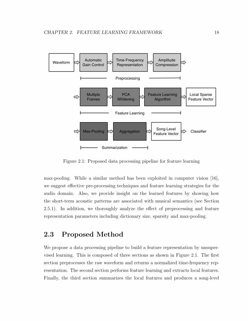
We propose a data processing pipeline to build a feature representation by unsuper-
vised learning. This is composed of three sections as shown in Figure 2.1. The first
section preprocesses the raw waveform and returns a normalized time-frequency rep-
resentation. The second section performs feature learning and extracts local features.
Finally, the third section summarizes the local features and produces a song-level

CHAPTER 2. FEATURE LEARNING FRAMEWORK 19
feature. Each block is detailed below.
2.3.1 Preprocessing
Musical signals are a highly variable and complex data. Ideally, we wish to have
feature-learning algorithm that capture all possible variations from the raw data (i.e.,
waveforms) without any preprocessing. In practice, however, appropriate peripheral
processing such as a time-frequency transform or normalization significantly helps
feature learning. In this section, we discuss time-frequency representations and sug-
gest normalization techniques to facilitate learning algorithms. Note that this section
somewhat uses acoustic knowledge or insight from it. However, we try to minimize it
by preserving the original input data intact as much as possible.
Automatic Gain Control
Sound is inherently dynamic. The constantly varying intensity and bandwidth in a
musical signal is a specific instance of this dynamism. The human hearing system
has a dynamic-range compression mechanism to control the level of incoming sounds.
This automatic gain control (AGC) is performed separately on each band of the
cochlear filter, thereby providing more regulated filter levels to auditory nerves [61].
Inspired by this auditory processing, we apply a time-frequency AGC as a front-end
preprocessing step.
The use of a time-frequency AGC assumes that a time-frequency representation
will be used as input data for feature-learning algorithms. In general, there is less
high-frequency energy than low-frequency energy in most classes of sounds, including
music due to timbral natures of sound sources or phase cancelation when mixing
multiple sources. As a result, high-frequency content is likely to be ignored by feature-
learning algorithm. A time-frequency AGC equalizes the spectral distribution so that
a learning algorithm can effectively capture dependencies in the spectral domain. In
addition to the spectral imbalance, the overall volume of sound files in a dataset
is usually not normalized because they are often obtained under different recording
conditions. As a byproduct, a time-frequency AGC regularizes the overall gain as

CHAPTER 2. FEATURE LEARNING FRAMEWORK 20
Input Spectrogram
kH
z
0 0.5 1 1.5 2 2.50
5
10
Sub−band Envelopes
kH
z
0 0.5 1 1.5 2 2.50
5
10
Equalized Spectrogram
Seconds
kH
z
0 0.5 1 1.5 2 2.50
5
10
−20
0
20
40
−40
−30
−20
−10
0
−20
0
20
40
Figure 2.2: Effect of a time-frequency Automatic Gain Control (AGC). The sub-bandenvelopes obtained from the original spectrogram are remapped to linear frequency(middle). This is used to equalize the original spectrogram (bottom). Note that thehigh-frequency content is boosted by the AGC in the output spectrogram.
well.
We used the time-frequency AGC proposed by Ellis [23]. It first computes an
FFT and maps the magnitude to a small number of sub-bands. Then it extracts
amplitude envelopes from each band using an envelope follower and remaps the sub-
band envelopes back to the linear-frequency scale as shown in the middle of Figure
2.2. Finally, it divides the original spectrogram by the remapped envelopes. As a

CHAPTER 2. FEATURE LEARNING FRAMEWORK 21
result, the time-frequency AGC equalizes input signals so that their energy spectrum
is more uniform, as shown in the bottom of Figure 2.2.
Time-frequency Representation
Musical sounds are generally characterized by harmonic or non-harmonic elements.
Thus, time-frequency transforms, whose basis functions are given as sinusoids, pro-
vide more interpretable representations of musical sounds. There are many choices
of time-frequency transforms such as STFT, constant-Q transform (more generally,
wavelet transform) and various filter banks. They are often modified by adapting
psycho-acoustic considerations. For example, the STFT is often mapped to percep-
tual frequency scales such as mel [99], Bark [113] and ERB [67] or to perceptual
amplitude levels such as loudness [97]. Constant-Q considers the perceptual aspect
by definition, that is, having higher frequency resolutions at lower frequencies. Some
filter banks are designed from scratch to imitate the cochlear responses in human ears
[84, 61].
In our data processing pipeline, we choose mel-frequency spectrogram as the pri-
mary time-frequency representation. The mel-frequency spectrogram is obtained from
spectrogram by mapping FFT frequency bins to a small number of mel frequency bins.
This emphasizes low-frequency content and squeezes high-frequencies into a smaller
number of bins as shown in Figure 2.3. There are two advantages of this frequency
mapping. First, it reduces the dimensionality of the data. This facilitates feature-
learning algorithms even with wide receptive fields, for example, if multiple frames
are used as input to the feature-learning algorithms (this will be explained in Section
2.3.2). Second, it alleviates unnecessarily detailed variations in the high frequency
content. In general, high-frequency content is statistically more variable or random.
The human ear is often agnostic to such details. Thus, high-frequency content is often
modeled as a wide sub-band energy in audio coding. The mel-frequency spectrogram
performs a similar mapping. Note that we chose a larger number of mel-frequency
bins in our experiments so that the reconstructed output from the mel-frequency spec-
trogram preserves the original quality as much as possible and thus the underlying
structure of the musical data can be discovered via feature-learning algorithms.

CHAPTER 2. FEATURE LEARNING FRAMEWORK 22
Equalized Spectrogram
kH
z
0 0.5 1 1.5 2 2.50
5
10
Mel−freq. Spectrogram
Seconds
Mel−
freq b
ins
0 0.5 1 1.5 2 2.5
20
40
60
80
100
120
−20
0
20
40
−40
−20
0
Figure 2.3: Comparison of (equalized) spectrogram and mel-frequency spectrogram.513 bins in spectrogram (FFT size is 1024) are mapped to 128 bins in mel-frequencyspectrogram.
Magnitude Compression
As a final preprocessing step, we compress the amplitude of the mel-frequency spec-
trogram using an approximate log scale, log10(1 + C|X(t, f)|), where |X(t, f)| is the
time-frequency representation and C controls the degree of compression [69]. In gen-
eral, the linear content of each bin of spectrogram or mel-frequency spectrogram
has an exponential distribution. Scaling with a log function makes it have a more
Gaussian-like distribution. This enables the magnitude to be well-fitted with PCA
whitening, which has an implicit Gaussian assumption.

CHAPTER 2. FEATURE LEARNING FRAMEWORK 23
2.3.2 Feature Learning: Common Properties
Now the input data is ready to be used for feature-learning algorithms. As previously
stated, the input data is pre-processed in a highly constrained manner so that it still
contains salient acoustic characteristics such as harmonic and transient distributions,
low and high energy, and their temporal dependency in the spectral domain. We
are going to capture the characteristic patterns with different unsupervised learn-
ing algorithms, for example, K-means, restricted Boltzmann machine, sparse coding,
auto-encoder and so forth. Although they perform the task using different mathemat-
ical schemes, their basic objective functions and meta parameters are shared. This
section discusses the common properties in a general perspective before introducing
individual algorithms. Firstly, we introduce PCA whitening used prior to feature
learning as another preprocessing step.1
PCA Whitening
PCA is a popular algorithm for reducing the dimensionality or removing pair-wise
correlation. PCA extracts a set of basis functions in a way that maximizes the
variance of the projected subspace. In this sense, it can be regarded as a feature-
learning algorithm. However, the basis functions are limited to be orthogonal and
thus it can learn only the second-order dependencies (a Gaussian distribution) of the
input data. For this reason, PCA is often used as a preprocessing step followed by
Independent Component Analysis (ICA) or other learning algorithms that capture
high-order dependency. With an additional normalizing step that makes the projected
space have unit variances, this processing is called PCA whitening [42]. Algorithm 1
describes the procedure to learn the transformation matrix for PCA whitening given
a matrix X where each column is a sample from input data. As a result, subtracting
the mean of X from each column of a new input data and multiply U′
performs
PCA whitening. Figure 2.4 shows an example of the PCA-whitened mel-frequency
1In a previous work, we placed PCA whitening in the pre-processing stage due to its rule inthe data processing pipeline [71]. However, we moved it to the feature-learning stage because thewhitening matrix is obtained in a data-driven manner similarly to other feature-learning algorithmsand, furthermore, PCA whitening itself is often used as a feature-learning algorithm [33].

CHAPTER 2. FEATURE LEARNING FRAMEWORK 24
Algorithm 1 PCA Whitening
1. Subtract the mean at each row of X. This returns a matrix X′
that has a zeromean for each row.
2. Compute the covariance matrix of X′
and perform eigen decomposition
X ′X ′T = UV UT , (2.1)
This returns the eigenvectors ui from each column of U and eigenvalues vi fromthe diagonal of V for i = 1, 2, 3...R where R is the input data dimension.
3. Choose ρ and find the maximum k such that
k∑i=1
vi
R∑i=1
vi
< ρ. This determines the
amount of dimensionality reduction.
4. Form a normalization (and diagonal) matrix D whose diagonal elements are1
vi+ε, where ε is a regularization parameter to prevent diagonal elements from
being excessively increased.
5. Multiply D and U , and define the output as U′. This is used as the whitening
matrix.
spectrogram.
Objective Function
Feature-learning algorithms commonly learn a basis functions, which is often called
a dictionary. They represent the input data with a linear combination of the basis
functions learned using the following objective function:
minD,s(i)
∑i
∥∥x(i) −Ds(i)∥∥22 (2.2)
where x(i) is an example of the input data, D is a matrix containing the basis functions,
and s(i) is an encoded feature vector based on the learned basis functions. In a
probabilistic setting, such as RBM, the objective function is described in a maximum

CHAPTER 2. FEATURE LEARNING FRAMEWORK 25
Figure 2.4: Mel-frequency spectrogram (top) and PCA-whitened mel-frequency spec-trogram (bottom). The figure indicates that 4 frames in the mel-frequency spectro-gram are chosen as a receptive field size and projected to a single vector in the PCAspace. The PCA indices are sorted such that components with high eigenvalues havelower index numbers.
likelihood form:
maxD
P (x|D) = maxD
∑h
P (x|D,h)P (h), (2.3)
where x is a random vector corresponding to the input data and h is a hidden random
vector that corresponds to s(i) above. This optimization problem is usually solved
by a type of bi-directional relaxation similar to Expectation-Maximization (EM).
This is described in Algorithm 2. Once we obtain the dictionary D, the feature
representations for new input data, for example, test data, can be calculated by
solving the second step above with fixed D.

CHAPTER 2. FEATURE LEARNING FRAMEWORK 26
Algorithm 2 Feature Learning Procedure
1. Initialize the basis functions D using either random numbers or randomly se-lected input data with appropriate normalization.
2. Fix D and solve Equation 2.2 to obtain s(i) or infer P (h|x, D) given x(i) inEquation 2.3.
3. Update D using the previous results. For example, solve the least squaresproblem given x(i) and fixed s(i)in Equation 2.2.
4. Repeat step 2 and 3 until the objective function converges.
Sparsity
In addition to the basic objective function defined in Equation 2.2 or 2.3, most feature-
learning algorithms have additional sparsity constraint on s(i) or h as this turns
out to be the core factor to be able to discover meaningful structures [12, 78, 96,
53]. Usually, an L1-norm or the mean of extracted feature vectors is used as an
additional regularization term. Specifically, the second step in Algorithm 2 includes
the additional sparsity term in the objective function.
Receptive Field Size
Receptive field originally refers to a region of space where the presence of a stimulus
changes the activity of a neuron in the human sensory system. In the feature-learning
context, this term is often used to indicate the input size from which a feature is
learned such as image patch size. In our setting, we select the receptive field from
the mel-frequency spectrogram. There are two aspects of the receptive field size: the
number of frames (time-wise) and the number of subbands (frequency-wise). The
number of frames is changed by selecting a different number of consecutive frames
along the time axis. Since neighboring frames in musical sounds tend to depend on
each other, for example, musical notes are usually sustained, the receptive field size
that covers multiple frames allows the system to learn temporal dependencies. The
number of subbands in the receptive field determines whether features are learned

CHAPTER 2. FEATURE LEARNING FRAMEWORK 27
separately for each subband or just once for a whole band. Using separate receptive
fields, however, may require an additional learning layer that captures dependency
among the sub-bands. In order to reduce complexity, we simply take the whole band
in our experiment. Figure 2.4 indicates the receptive field size and shows how multiple
frames of the mel-frequency spectrogram are used as input to the learning algorithm.
Dictionary Size
Dictionary size refers to the number of the basis functions. This is also called feature
size or hidden layer size in different algorithms or contexts. Dictionary size is one of
the most important meta parameters of learning algorithms because it directly deter-
mines the diversity of learned features in single-layer algorithms and also corresponds
to the input dimension of the classifier in our pipeline. In general, a large number
of dictionary size is preferred in single-layer algorithms as it significantly influences
classification performance [16].
2.3.3 Feature Learning: Algorithms
This section describes individual feature-learning algorithms that we evaluated in our
experiment.
K-means Clustering
K-means clustering is a well-known unsupervised learning algorithm. It learns K
cluster and their centroids from the input data and assigns the membership of a
given input to one of the K clusters. The training is performed by alternating two
steps:
1. Compute distances between data examples and the current centroids and find
the nearest centroids for each data example.
2. Update centroids with the mean of the examples assigned to each centroid.
As a result, given a set of centroids, K-means performs a hard assignment as follow:

CHAPTER 2. FEATURE LEARNING FRAMEWORK 28
fk(x) =
1 if k = argminj||x− c(j)||220 otherwise .
(2.4)
This computation is exactly the same as steps 2 and 3 of Algorithm 2 if a set
of K centroids is regarded as a dictionary and the membership is represented as an
extremely sparse feature vector s that has all zeros except a single “1” corresponding
to the assigned centroid. For example, if K is 5 and an example is closest to the 1st
centroid, the feature vector s will be represented as [1 0 0 0 0]. In this sense, K-means
can be regarded as having a sparsity constraint by nature, specifically, providing the
maximally sparse representation.
K-means Clustering: Soft Encoding
Coates et. al. recently used a variation of K-means encoding, noting that the hard
assignment by K-means makes the feature vector too terse [16]. Given a set of cen-
troids (learned using the K-means clustering), the new encoding method performs
a non-linear mapping that attempts to be “gentler” while maintaining sparsity as
follows:
fk(x) = max(0, µ(z)− zk), (2.5)
where zk = ||x − c(k)||2 and µ(z) is the mean of the elements of z. This encoding
returns 0 for any feature fk where the distance to the centroid c(k) is “above average,”
thereby setting half the elements of the feature vector s to zero. They showed that this
simple tweaking of the encoding significantly improve image recognition performance.
We refer to this soft encoding as K-means (soft) and the hard assignment version as
K-mean (hard).
Sparse Coding
Sparse coding is an unsupervised learning algorithm to represent input data efficiently
with a set of basis functions that we call a dictionary. The goal of sparse coding is
to find a dictionary such that an input vector x ∈ Rn is represented as a linear

CHAPTER 2. FEATURE LEARNING FRAMEWORK 29
combination of the dictionary elements:
x =k∑j=1
sjdj , (2.6)
where dj is a dictionary element vector and sj is the corresponding coefficient. The
dictionary size k is often set to be greater than input dimensionality n, rendering
Equation 2.6 an over-complete representation. However, with this condition (k >
n), the coefficients s are no longer uniquely determined. Therefore, an additional
constraint called sparsity is introduced to resolve this problem. Ideally, an L0 norm
of the coefficients s, the number of non-zero values, is used as sparsity constraint.
However, it is not differentiable and difficult to optimize in general, and is known
to be NP-hard. Instead, the L1 norm of the coefficients s, is commonly used as a
relaxation. As a result, a dictionary to build a over-complete representation is learned
using the following objective function:
minD,s(i)
∑i
∥∥Ds(i) − x(i)∥∥22
+ λ∥∥s(i)∥∥
1, (2.7)
where D is the dictionary matrix si is the sparse code and λ controls the amount of
sparsity. In addition, the dictionary D is constrained to be normalized such that, for
each dictionary element, ‖dj‖22 = 1.
There are many algorithms to find the dictionary and sparse code. They are all
based on the alternating minimization rule in Section 2.3.2. Specifically, the second
step, which finds sparse code s(i) given a dictionary D, is called the L1 minimization
problem or inference step in the probabilistic context:
mins(i)
∑i
∥∥Ds(i) − x(i)∥∥22
+ λ∥∥s(i)∥∥
1. (2.8)
The third step, which updates the dictionary given the inferred sj, is formed as a

CHAPTER 2. FEATURE LEARNING FRAMEWORK 30
least squares problem, often with a unit L2 norm constraint for dj:
minD
∑i
∥∥Ds(i) − x(i)∥∥22
subject to ‖dj‖22 = 1, ∀j.(2.9)
Following Coates [17], we solved the L1 minimization problem using a coordinate
descent algorithm [110] and the least squares problem simply using a inverse of the
dictionary matrix followed by the unit normalization. After we learn the dictionary,
we use the absolute value of the sparse code s(i) as learned features to incorporate it
into the max-pooling and aggregation stage.
Auto-Encoder
Auto-encoder is an unsupervised neural network algorithm where the output is con-
figured to reconstruct the input [74, 37, 4]. A single-layer neural network is described
as follows:
h(i) = g(W1x(i) + b1) (2.10)
y(i) = W2h(i) + b2 , (2.11)
where x is the input data, h is the hidden layer output, y is the output, W1 and W2
are network parameters, b1 and b2 are bias terms, and g(z) = 1/(1 + exp(−z)) is the
logistic sigmoid function. The auto-encoder is trained to minimize the reconstruction
error:
E(W1,W2, b1, b2) =∑i
∥∥y(i)(x(i))− x(i)∥∥2, (2.12)
where W1 and W2 are often tied to be transpose to each other, that is, W T1 = W2.
In addition, we introduce a constraint on the hidden layer to promote sparsity.
We use the KL divergence between a target activation ρ and the mean activation ρj

CHAPTER 2. FEATURE LEARNING FRAMEWORK 31
for the hidden layer [74]:
K∑j=1
KL(ρ||ρj) =K∑j=1
ρ logρ
ρj+ (1− ρ) log
1− ρ1− ρj
(2.13)
where ρj = 1m
m∑i=1
h(x(i)). This way, sparsity is controlled by setting a small value to
the target activation. Finally, the sparse auto-encoder is trained by minimizing the
sum of the reconstruction error and the KL divergence:
minW1,W2
E ′(W1,W2, b1, b2) = minW1,W2
E(W1,W2, b1, b2) +K∑j=1
KL(ρ||ρj) . (2.14)
This is usually solved by gradient descent because both terms are differentiable with
regard to the network parameters and bias terms:
W1 ← W1 + µ∂E ′(W1,W2, b1, b2)
∂W1
(2.15)
W2 ← W2 + µ∂E ′(W1,W2, b1, b2)
∂W2
(2.16)
b2 ← b1 + µ∂E ′(W1,W2, b1, b2)
∂b1(2.17)
b2 ← b2 + µ∂E ′(W1,W2, b1, b2)
∂b2, (2.18)
where µ is the learning rate.
Note that W2 plays a role of feature bases in feature-learning context and h(i)(x(i))
is the learned features.
Restricted Boltzmann Machine
A restricted Boltzmann Machine (RBM) is a probabilistic version of the auto-encoder.
The RBM is defined as a bipartite undirected graphical model as shown in Figure 2.5

CHAPTER 2. FEATURE LEARNING FRAMEWORK 32
[98]. It consists of visible nodes x and hidden nodes h where the visible nodes repre-
sent input vectors and the hidden nodes represent the features learned by training the
RBM. The joint probability for the hidden and visible nodes is defined in Equation
2.19 when the visible notes are real-valued Gaussian units and the hidden notes are
binary units. The RBM has symmetric connections between the two layers denoted
by a weight matrix W , but no connections within the hidden nodes or visible nodes.
This particular configuration makes it easy to compute the conditional probability
distributions, when nodes in either layer are observed (Equation 2.20 and 2.21).
− logP (x,h) ∝ E(x,h) =1
2σ2xTx− 1
σ2
(cTx + bTh + hTWx
)(2.19)
p(hj|x) = g(1
σ2(bj + wT
j x)) (2.20)
p(xi|h) = N ((ci + wTi h), σ2), (2.21)
where σ2 is a scaling factor, b and c are bias terms, and W is a weight matrix. The
parameters are estimated by maximizing the log-likelihood of the visible nodes. This
is approximated by block Gibbs sampling between two layers, particularly, using the
contrastive-divergence learning rule which involves only a single iteration of Gibbs
sampling [36].
x1 x2 x3
h1 h2 h3 h4
W
b
c
Figure 2.5: Undirected graphical model of a RBM.
We further regularize this model with a sparsity term by encouraging each hidden

CHAPTER 2. FEATURE LEARNING FRAMEWORK 33
unit to have a pre-determined expected activation using a regularization penalty:
∑j
(ρ− 1
m(m∑l=1
E[hj|xl]))2, (2.22)
where {x1, ...,xm} is the training set and ρ determines the target sparsity of the hidden
unit activations [53]. This term is added to the maximum-likelihood estimation.
Finally, the parameters are obtained from the following optimization problem:
minW,b,c
m∑l=1
− log∑h
P (x,h) + λ∑j
(ρ− 1
m(m∑l=1
E[hj|xl]))2 (2.23)
Similarly to the sparse auto-encoder, we can interpret W as a dictionary and h as
sparse code. Also, both the auto-encoder and the RBM do not need any iterative com-
putation because they have an explicit encoding scheme h = g( 1σ2 (b + W Tx)). This
property is particularly useful in real-time applications because the feature can be ex-
tracted using a simple feed-forward computation. Figure 2.3 shows a mel-frequency
spectrogram and the corresponding hidden-layer activation. Note that the encoded
feature representation is very sparse compared to the mel-frequency spectrogram (only
1% of hidden units are activated in this example).
2.3.4 Feature Summarization
Max-Pooling and Aggregation
The feature-representation algorithms provide sparse feature vectors for short-term
frames. Since a song is a very long sequence of data, however, we need to summarize
them to construct a song-level feature. A typical approach is aggregating them as a
histogram, that is, by averaging them over a song or a song segment. [32, 35]. How-
ever, averaging every single short-terms feature can dilute their local discriminative
power. Therefore, we first perform pooling to find only dominant features over a
small segment and then aggregate the output over a song.
Pooling summarizes local features obtained at neighboring locations into a group
of statistic that is often called a bag of features (BoF) [10]. For example, Hamel et.

CHAPTER 2. FEATURE LEARNING FRAMEWORK 34
Mel−freq. Spectrogram
Seconds
Me
l−fr
eq
bin
s
0 0.5 1 1.5 2 2.5
20
40
60
80
100
120
−40
−20
0
Feature Bases
Hidden Layer Index
Me
l−fr
eq
bin
s
20
40
60
80
100
120
−1
−0.5
0
0.5
1
Hidden Layer Activation
Seconds
Hid
de
n L
aye
r In
de
x
0 0.5 1 1.5 2 2.5
50
100
150
200
250
0.2
0.4
0.6
0.8
Figure 2.6: Comparison of mel-frequency spectrogram and the learned feature repre-sentation (hidden layer activation) using sparse RBM. The dictionary size was set to1024 and target activation (sparsity) was to 0.01. That means that only 1% out of1024 features are activated on average.

CHAPTER 2. FEATURE LEARNING FRAMEWORK 35
al evaluated various types of pooling such as mean, min, max, variance and other
high-order statistics and their combinations on PCA-whitened frame-level features
for music tag classification [33]. We perform max-pooling by taking the maximum
value at each dimension over a segment. Max-pooling is often used in convolutional
neural networks to reduce feature scales and also make them invariant to local shifts.
In our experiment, max-pooling works as a form of temporal masking because it
discards small details around a high peak of feature activation. Figure 2.7 compares
the hidden layer activation obtained by training sparse RBM with its max-pooled
version. This shows that max-pooling removes small noisy feature activation and
makes peaks more distinct. The max-pooled features are summed over a song as a
histogram of dominant feature activations. This summarization eventually provides
a single song-level feature vector.
2.3.5 Classification
The feature representation data processing pipeline produces a single feature vector
for a song. They are used for a classifier that performs supervised training where a
single or multiple labels are given. In our experiment, we use a linear support vector
machine (SVM) as a reference classifier to evaluate the feature representations learned
by different algorithms and parameters. The linear SVM is trained by minimizing a
L2-regularized L2 hinge loss given the training data [28]:
minw
M∑j=1
(1
2wTj wj + C
N∑i=1
max(0, 1− y(i)j wTj x(i)))2 , (2.24)
where wj is SVM parameter, C is a regularization weight, x(i) is the song-level fea-
ture vector augmented with ’1’ for the bias term, y(i)j ∈ {−1, 1} is the label and j
corresponds to one of the M output classes. After training, we make predictions by
choosing j that produces the maximum value of wTj x(i). We implemented the SVM
using the publicly available Matlab optimization library, minFunc.2
2Matlab library found in http://www.cs.ubc.ca/~schmidtm/Software/minFunc.html

CHAPTER 2. FEATURE LEARNING FRAMEWORK 36
05
1015
20
0
5
10
15
200
0.5
1
Seconds
Hidden Layer Activation
Hidden Layer Index
05
1015
20
0
5
10
15
200
0.5
1
SecondsHidden Layer Index
Figure 2.7: Comparison of hidden layer activation and its max-pooled version. Forvisualization, the hidden layer features masked by the maximum value in their poolingregion were set to zero. As a result, the max-pooled feature maintains only locallydominant activation. The hidden layer feature representation was learned using sparseRBM. Dictionary size was set to 1024, sparsity was to 0.01 and max-pooling size wasto 43 frames (about 1 second).

CHAPTER 2. FEATURE LEARNING FRAMEWORK 37
2.4 Experiments
2.4.1 Datasets
We evaluated our proposed feature representation on two popularly used genre datasets:
GTZAN and ISMIR2004.
GTZAN
GTZAN is a public music genre dataset released by Tzanetakis [104]. This has been
used as a benchmark dataset to evaluate genre classification algorithms [80, 58, 62, 5,
51, 82, 83, 29, 6, 45]. Recent work based on feature-learning algorithms also evaluated
these methods on this dataset [32, 35]. GTZAN contains 10 different genres and 100
song segments evenly for each genre: Blues, Classical, Country, Disco, Hiphop, Jazz,
Metal, Pop, Reggae, and Rock. All song segments are 30-second long.
ISMIR2004
ISMIR2004 is another publicly available genre dataset released after the MIREX 2004
competition.3 This contains 6 different genres: Classical (320 samples), Electronic
(115 samples), Jazz/Blues (26 samples), Metal/Punk (45 samples), Rock/Pop (101
samples), and World (122 samples). Each sample has the full length of a song. In
this experiment, we took only a 30-second segment after the first 30 seconds of each
song. This dataset has been also a secondary benchmark dataset to evaluate genre
classification algorithms [59, 79, 39, 82].
2.4.2 Preprocessing Parameters
We first resampled the waveform data to 22.05kHz and computed an FFT with a 46ms
Hann window and 50% overlap. This produces a 513 dimensional vector (up to half
the sampling rate) for each frame. As for the time-frequency AGC, we mapped the
spectrogram to 10 sub-bands and calculated each envelope using temporal smoothing.
3http://ismir2004.ismir.net/genre_contest/index.htm

CHAPTER 2. FEATURE LEARNING FRAMEWORK 38
After equalizing the spectrogram with the envelopes (by remapping them back to the
spectrogram domain), we then converted the output to a mel-frequency spectrogram
with 128 bins. In the magnitude compression, the strength C was fixed to 10.
2.4.3 Feature-Learning Parameters
We sampled 100,000 data examples at random positions for each dataset for PCA
whitening and subsequent feature learning. The receptive field was selected as a
128 × n (n=1, 2, 4 and 6) patch from the preprocessed data. In PCA whitening,
we reduced the dimensionality of the sampled data by retaining 90% of the variance.
Before the whitening, we added 0.01 to the variance for regularization. We used
dictionary size (or hidden layer size) and sparsity (when applicable) as the primary
feature-learning parameters. The dictionary size was varied over 128, 256, 512, 1024
and 2048. The sparsity parameter was set to ρ = 0.005, 0.007, 0.01, 0.02, 0.03 and
0.05 for sparse RBM and sparse Auto-Encoder and λ = 1.0, 1.5, 2.0 and 2.5 for sparse
coding. Then, max-pooling was performed over segments of length 0.1, 0.25, 0.5, 1,
2, 4, 8 and 16 seconds.
2.4.4 Classifier Parameters
We first standardized the song-level features obtained from the feature representation
stage by subtracting the mean and dividing by the standard deviation of those in the
training set. We fixed a classifier to a linear Support Vector Machine (SVM) in
order to focus only on evaluation features. In GTZAN, we performed 10-fold cross-
validation following the practice of previous work. In ISMIR2004, we used the original
split between training, development and test sets.

CHAPTER 2. FEATURE LEARNING FRAMEWORK 39
2.5 Evaluation
2.5.1 Visualization
We show feature bases learned by the sparse RBM in Figure 2.6. While the majority
of previous work show such feature bases patterns captured by different feature-
learning algorithms, there are few attempt to associate them with high-level musical
semantics such as genre. We suggest a systematic way to find the relationship and
better understand the learned features. This is performed by finding the top-K active
feature bases given a genre label as follows:
1. Select a subset of the dataset that belong to a specific genre.
2. Given learned feature bases, compute feature representations of the subset.
3. Summarize all the local features using a histogram.
4. Sort the histogram in descending order and choose the top-K elements that have
the highest values.
5. Repeat the steps above for each genre.
This returns the most actively triggered K feature bases for the music genre. Figure
2.8 shows the most active top-20 feature bases learned on GTZAN for ten music
genres (one for sparse RBM and the other for sparse coding). The correspond-
ing feature bases are vividly distinguished by different timbral patterns, such as
harmonic/non-harmonic, wide/narrow band, strong low/high-frequency content and
steady/transient ones. Different genres of music trigger specific types of feature bases
more actively than others. For example, classical and jazz music mainly trigger
harmonic features. Metal music is likely to have more high-frequency energy and
wide-band patterns. In addition, disco, reggae and hiphop music contain significant
portions of transient patterns. This indicates the feature-learning algorithms effec-
tively encode the input data into high-dimensional sparse feature vectors such that
the feature vectors are “selectively” activated by a given genre of music.
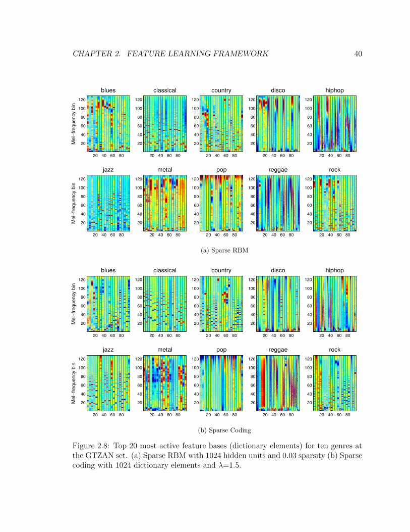
CHAPTER 2. FEATURE LEARNING FRAMEWORK 40
blues
Mel−
frequency b
in
20 40 60 80
20
40
60
80
100
120
classical
20 40 60 80
20
40
60
80
100
120
country
20 40 60 80
20
40
60
80
100
120
disco
20 40 60 80
20
40
60
80
100
120
hiphop
20 40 60 80
20
40
60
80
100
120
jazz
Mel−
frequency b
in
20 40 60 80
20
40
60
80
100
120
metal
20 40 60 80
20
40
60
80
100
120
pop
20 40 60 80
20
40
60
80
100
120
reggae
20 40 60 80
20
40
60
80
100
120
rock
20 40 60 80
20
40
60
80
100
120
(a) Sparse RBM
blues
Mel−
frequency b
in
20 40 60 80
20
40
60
80
100
120
classical
20 40 60 80
20
40
60
80
100
120
country
20 40 60 80
20
40
60
80
100
120
disco
20 40 60 80
20
40
60
80
100
120
hiphop
20 40 60 80
20
40
60
80
100
120
jazz
Mel−
frequency b
in
20 40 60 80
20
40
60
80
100
120
metal
20 40 60 80
20
40
60
80
100
120
pop
20 40 60 80
20
40
60
80
100
120
reggae
20 40 60 80
20
40
60
80
100
120
rock
20 40 60 80
20
40
60
80
100
120
(b) Sparse Coding
Figure 2.8: Top 20 most active feature bases (dictionary elements) for ten genres atthe GTZAN set. (a) Sparse RBM with 1024 hidden units and 0.03 sparsity (b) Sparsecoding with 1024 dictionary elements and λ=1.5.

CHAPTER 2. FEATURE LEARNING FRAMEWORK 41
2.5.2 Results and Discussion
We analyze genre classification accuracy for different preprocessing options and meta
parameters of learning algorithms.
Spectrogram versus mel-frequency spectrogram
Figure 2.9 compares the linear spectrogram and mel-frequency spectrogram as the
input time-frequency representation. We compare different receptive field sizes for
both the sparse RBM and sparse coding. The mel-frequency spectrogram outper-
forms the linear spectrogram for all cases. This confirms that high frequency content
tends to have unnecessary details and thus squeezing them (as done by mel-frequency
spectrogram) helps the learning algorithm focus on the more important variations.
In addition, since the mel-frequency spectrogram has a much smaller size (by 4 times
in the experiment), it is computationally more efficient.
1 2 3 4 5 670
75
80
85
90
95
Number of frames
Accu
racy [
%]
spec
mel−spec
(a) RBM
1 2 3 4 5 670
75
80
85
90
95
Number of frames
Accu
racy [
%]
spec
mel−spec
(b) Sparse Coding
Figure 2.9: Comparison of spectrogram and mel-frequency spectrogram. The dictio-nary size is set to 1024.

CHAPTER 2. FEATURE LEARNING FRAMEWORK 42
Effect of Automatic Gain Control (AGC)
Figure 2.10 shows the effect of the time-frequency AGC for different receptive field
sizes. Again, they are compared separately for the sparse RBM and sparse coding.
For both feature-learning algorithms, the AGC consistently increases the accuracy by
about 2 ∼ 5% regardless of the receptive field size.
1 2 3 4 5 670
75
80
85
90
95
Number of frames
Accu
racy [
%]
no AGC
AGC
(a) RBM
1 2 3 4 5 670
75
80
85
90
95
Number of frames
Accu
racy [
%]
no AGC
AGC
(b) Sparse Coding
Figure 2.10: Effect of Automatic Gain Control. The dictionary size is set to 1024.
Effect of Receptive Field Size
Figure 2.11 compares the results for different receptive field sizes and separately for
five feature-learning algorithms. In general, accuracy increased when multiple frames
were chosen. This indicates that learning temporal dependencies indeed helps to
discriminate different genres. However, as the receptive field size increases, the result
becomes saturated from the four frames. This is expected at some point because
variations in the receptive field grow exponentially and thus learning algorithms are
no longer capable of capturing the variations. Among the five algorithms, sparse
coding outperforms the others for all sizes. It is notable that K-means (hard) get

CHAPTER 2. FEATURE LEARNING FRAMEWORK 43
1 2 4 675
80
85
90
Number of frames
Accura
cy [%
]
SC
RBM
Kmeans(hard)
Kmeans(tri)
AE
Figure 2.11: Effect of receptive field size. The dictionary size is set to 1024.
degraded as the numbers of frames increases whereas K-means (soft) is comparable
to other algorithms that have sparsity control. This may be related to the lack of
sparsity control, that is, too extreme fixed sparsity in K-mean (hard).
Dictionary Size and Sparsity
Dictionary size is one of the most crucial parameters because it determines not only
diversity of the feature patterns but also the input dimension of the classifier that
follows in our data processing pipeline. This is illustrated in Figure 2.12. The ac-
curacy dramatically increases as the dictionary size increases from 128 to 1024 and
saturates by 2048. In addition, Figure 2.13 shows how the sparsity affects perfor-
mance for each dictionary size and separately with regard to the RBM and sparse
coding. In the RBM, sparsity is controlled by a target activation for the hidden layer
units. Thus, as the sparsity value decreases, hidden layer activation, that is, feature
representations become sparser. In sparse coding, sparsity is controlled as a weight
for sparsity constraint (i.e., L1 norm of the feature activation). Thus, as the weight

CHAPTER 2. FEATURE LEARNING FRAMEWORK 44
128 256 512 1024 204872
74
76
78
80
82
84
86
88
90
Dictionary Size [sec]
Accura
cy [%
]
SC
RBM
Kmeans(hard)
Kmeans(tri)
AE
Figure 2.12: Effect of dictionary size. The receptive field size is set to 4 frames.
(λ) increases, the feature vectors become sparser. The plots show a relation between
optimal sparsity and dictionary size. For small dictionary sizes, the accuracy tends
to be higher when the features are relatively less sparse. For large dictionary sizes, on
the other hand, the accuracy tends to be higher when they are sparser. As a result,
the best genre-classification accuracy is achieved by “high-dimensional sparse feature
representations.”
Max-pooling Size
Figure 2.14 plots the results for different max-pooling sizes with regard to two dictio-
nary sizes, 512 and 2048. In general, as the max-pooling size becomes larger, accuracy
increases up to a point and then decreases after that. Compared to the point where
max-pooling is not performed (the leftmost one), the peak classification performance
gains 6 ∼ 7 % accuracy improvement, showing that max-pooling is a very effective
technique to boost discriminative power. Another noticeable result is that the optimal
max-pooling size depends on the dictionary size. For example, when the dictionary
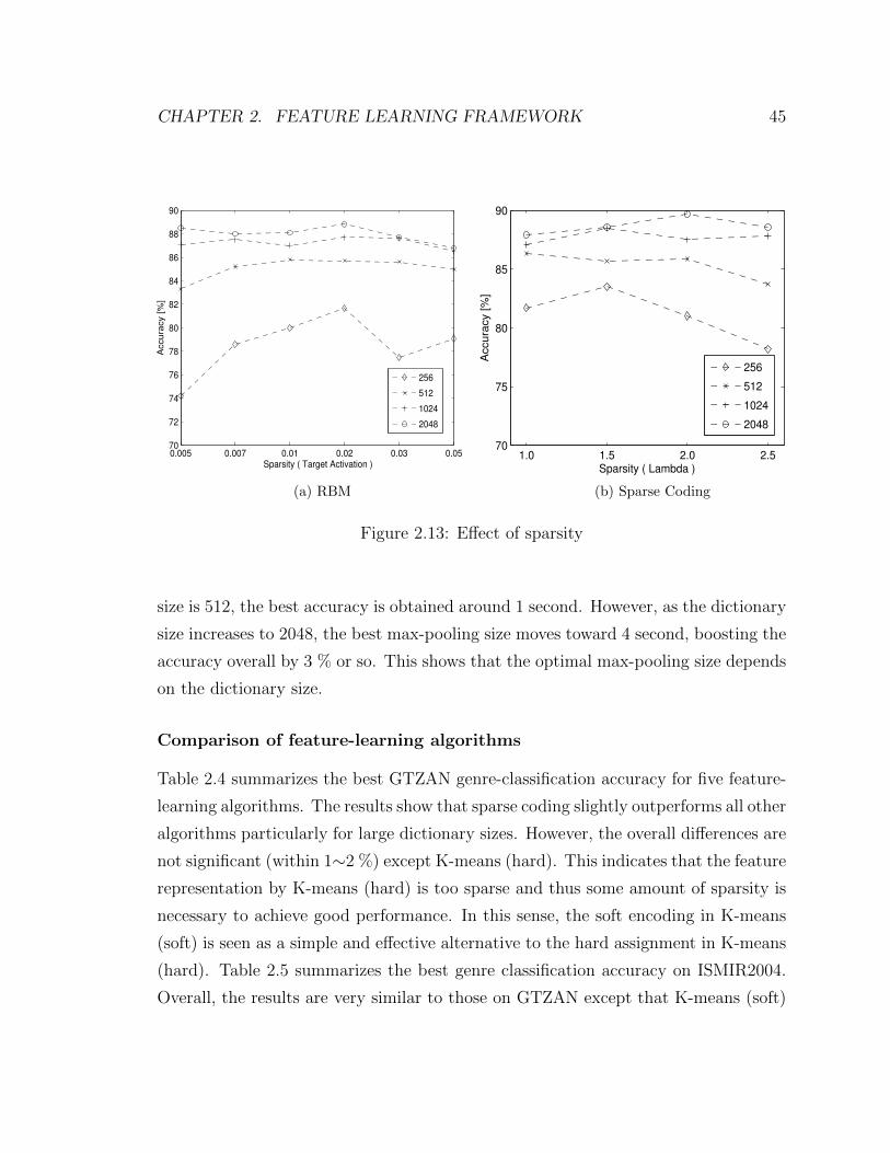
CHAPTER 2. FEATURE LEARNING FRAMEWORK 45
0.005 0.007 0.01 0.02 0.03 0.0570
72
74
76
78
80
82
84
86
88
90
Sparsity ( Target Activation )
Accu
racy [
%]
256
512
1024
2048
(a) RBM
1.0 1.5 2.0 2.570
75
80
85
90
Sparsity ( Lambda )
Accu
racy [
%]
256
512
1024
2048
(b) Sparse Coding
Figure 2.13: Effect of sparsity
size is 512, the best accuracy is obtained around 1 second. However, as the dictionary
size increases to 2048, the best max-pooling size moves toward 4 second, boosting the
accuracy overall by 3 % or so. This shows that the optimal max-pooling size depends
on the dictionary size.
Comparison of feature-learning algorithms
Table 2.4 summarizes the best GTZAN genre-classification accuracy for five feature-
learning algorithms. The results show that sparse coding slightly outperforms all other
algorithms particularly for large dictionary sizes. However, the overall differences are
not significant (within 1∼2 %) except K-means (hard). This indicates that the feature
representation by K-means (hard) is too sparse and thus some amount of sparsity is
necessary to achieve good performance. In this sense, the soft encoding in K-means
(soft) is seen as a simple and effective alternative to the hard assignment in K-means
(hard). Table 2.5 summarizes the best genre classification accuracy on ISMIR2004.
Overall, the results are very similar to those on GTZAN except that K-means (soft)

CHAPTER 2. FEATURE LEARNING FRAMEWORK 46
0.023 0.1 0.25 0.5 1 2 4 8 1675
80
85
90
Max−pooling [sec]
Accu
racy [
%]
SC
RBM
Kmeans(hard)
Kmeans(tri)
AE
(a) dictionary size = 512
0.023 0.1 0.25 0.5 1 2 4 8 1675
80
85
90
Max−pooling [sec]
Accu
racy [
%]
SC
RBM
Kmeans(hard)
Kmeans(tri)
AE
(b) dictionary size = 2048
Figure 2.14: Effect of max-pooling
achieves outstanding accuracy for small dictionary sizes.
While sparse coding is slightly superior in terms of accuracy to other algorithms,
the encoding in sparse coding requires iterative computation steps to solve the L1
minimization. This slows down feature extraction for new input in the testing phase,
prohibiting it from being used in real-time applications 4. On the other hand, sparse
RBM and auto-encoder have an explicit encoding scheme that has a single feed-
forward computation step. K-means also can extract features simply by computing
distances from centroids. Thus, these algorithms are more useful when real-time
processing is required or computation resources are limited.
In terms of training time or complexity, auto-encoder and RBM were most difficult
to train because they need a number of hyper-parameters and cross-validating all of
the meta parameters can be time-consuming. Thus, we fixed several hyper-parameters
(e.g., weight cost and scale) to a constant after finding appropriate values in our initial
experiments. On the other hand, K-means clustering (both hard and soft encoding)
4A variant of sparse coding, called Predictive Sparse Coding [47], has a separate encoding schemeto overcome this problem.

CHAPTER 2. FEATURE LEARNING FRAMEWORK 47
Algorithms Best Accuracy (%)
Dictionary Size 128 256 512 1024 2048
K-mean (hard) 75.9 79.6 82.6 85.1 86.0
K-mean (soft) 78.5 82.2 84.7 86.6 88.4
Sparse RBM 74 81.7 85.8 87.7 88.8
Sparse Auto-encoder 79.2 83.3 85.9 87.4 88.8
Sparse Coding 77.1 83.5 86.3 88.5 89.7
Table 2.1: Comparison of different feature-learning algorithms on the GTZAN genredataset.
requires only a single parameter (dictionary size) and the training algorithm is simple
and fast as well. Therefore, the K-means, especially with soft encoding, is seen to be
the most efficient solution for feature learning in this regard.
Confusion Matrix
Table 2.3 shows a confusion matrix for the best accuracy obtained with sparse coding
on GTZAN. Classical, blues, jazz and metal have high accuracy, above 94 %, whereas
country, disco and rock have relatively low accuracy. In particular, rock is significantly
lower than others, being confused mainly with country and metal. This makes sense
because rock is used as a broad musical category and the three genres share a guitar
in common. Other incorrect results also occur among relatively similar genres, for
example, disco and pop. The low accuracy in disco and reggae can be explained
by the lack of rhythmic feature extraction in our method. Although the song-level
feature implicitly captures rhythmic characteristic by averaging activation of transient
patterns (usually appearing in note onsets), this seems to be not sufficient to capture
the sophisticated rhythms in disco or reggae.

CHAPTER 2. FEATURE LEARNING FRAMEWORK 48
Algorithms Best Accuracy (%)
Dictionary Size 128 256 512 1024 2048
K-mean (hard) 77.8 79.6 82.0 82.17 83.4
K-mean (soft) 81.9 83.8 84.5 85.7 86.1
Sparse RBM 77.4 81.9 83.8 85.0 85.7
Sparse Auto-encoder 79.5 82.3 84.6 85.0 84.9
Sparse Coding 79.4 81.8 84.6 85.7 86.8
Table 2.2: Comparison of different feature-learning algorithms on the ISMIR2004genre dataset.
Blues Classical Country Disco Hiphop Jazz Metal Pop Reggae Rock
Blues 94 1 2 1 0 2 0 0 0 0
Classical 0 99 1 0 0 0 0 0 0 0
Country 1 2 86 2 0 0 0 2 1 6
Disco 0 0 2 87 3 1 1 2 1 3
Hiphop 0 0 1 2 88 0 3 4 2 0
Jazz 1 4 0 0 0 94 1 0 0 0
Metal 0 0 0 1 0 0 97 0 0 2
Pop 0 0 2 3 0 0 1 90 3 1
Reggae 0 0 1 2 3 1 0 1 89 3
Rock 1 0 11 3 0 2 5 2 3 73
Table 2.3: Confusion Matrix for ten genres for the best algorithm (sparse coding gives89.7% accuracy) on the GTZAN gene dataset.

CHAPTER 2. FEATURE LEARNING FRAMEWORK 49
Classifiers Features Accuracy (%)
CSC Many hand-engineered features [45] 92.7
SRC Auditory temporal modulations [81] 92
Linear SVM Proposed method (sparse coding) 89.7
Linear SVM Learned using K-means [111] 85.3
RBF-SVM Learned using deep belief network [34] 84.3
Linear SVM Learned using predictive sparse coding [35] 83.4
AdaBoost Many hand-engineered features [5] 83
SVM Daubechies Wavelet Coefficients [58] 78.5
Log. Regression Spectral Covariance [6] 77
Linear SVM Auditory Temporal Modulations [81] 70
GMM Many hand-engineered features [104] 61
Table 2.4: Comparison with state-of-the-art algorithms on the GTZAN genre dataset
Classifiers Features Accuracy (%)
SRC Auditory temporal modulations [81] 93.6
Linear SVM Proposed method (sparse coding) 86.8
GMM NMF-based features [39] 83.5
NearestNeighbor Spectral Similarity / fluctuation patterns [79] 82.3
RBF-SVM Auditory temporal modulations [82] 81.0
Linear SVM Many hand-engineered features [59] 79.7
Table 2.5: Comparison with state-of-the-art algorithms on the ISMIR2004 genredataset
CHAPTER 2. FEATURE LEARNING FRAMEWORK 50
Comparison to state-of-the-art algorithms
Table 2.4 and 2.5 compare our best accuracy with previous results on GTZAN and
ISMIR2004, respectively. State-of-the-art algorithms achieved greater than 90% on
both datasets using hand-engineered features. However, they use complicated non-
linear classifiers. On the other hand, our result is the third from the top using only
using a linear classifier. Among those based on feature learning, we achieved the
highest accuracy, which is 4.4% greater than the second (85.3 %) or 5.4 % greater
than the deep learning method with a non-linear classifier (84.3 %)
2.6 Conclusion
We presented a data processing pipeline to learn high-dimensional sparse features
from a short-term receptive field on mel-frequency spectrogram and summarize them
to form a song-level feature vector. We showed that the framework can effectively
capture manifold acoustic patterns such as harmonic/non-harmonic, steady/transient,
low/high-frequency energy and wide/narrow band. As the learned patterns are se-
lectively activated for different genres of music due to the sparsity constraint, we can
regard them as low-level musical neurons.
We also conducted comprehensive analysis on how each processing module af-
fects performance. The results show that, while there are small degrees of differences
among feature-learning algorithms, the use of time-frequency AGC, log-frequency
scale (as in mel-frequency spectrogram) and meta parameters (e.g., receptive field
size, dictionary size and max-pooling size) significantly improve classification accu-
racy. This indicates that, in order to achieve good performance, appropriate prepro-
cessing, high-dimensional feature learning and dominant feature selection (by sparsity
and max-pooling) are of paramount importance over using different feature-learning
algorithms.
Finally, we compared our method to previous state-of-the-arts based on hand-
crafted features or feature learning. The results show that, with a simple linear
classifier, our approach achieved high accuracy comparable to the top group and the

CHAPTER 2. FEATURE LEARNING FRAMEWORK 51
best accuracy among those based feature learning on the GTZAN and ISMIR2004
datasets.

Chapter 3
Music Annotation and Retrieval
Using Feature Learning
3.1 Introduction
We presented a feature representation framework and applied it to music genre classi-
fication in Chapter 2. Genre is the most commonly used and acknowledged categorical
concept to distinguish different kinds of music. Thus, the majority of music service
providers organize the music content based on genre so that users can conveniently
browse the music collection. As such, automatic genre classification has been one of
the most popular topics in MIR research.
However, many criticize the inconsistency and ambiguity of genre labels. A genre
usually has a number of sub-genres and they are often created by fusing different
genres. This makes the taxonomy of genre hierarchical and somewhat entangled.
Thus, a song can be recognized as different genres or having multiple genres [65]. Also,
some genre decisions are based upon the extrinsic descriptions of music, for example,
artist’s overall musical characteristic (even if individual songs belong to different
genres), locality of the artists home country or languages and other cultural signals,
rather than the intrinsic musical attributes such as rhythm, timbre or tonality. For
these reasons, it has been argued that the 1-of-K classification problem for automatic
genre classification is an ill-defined problem [2].
52
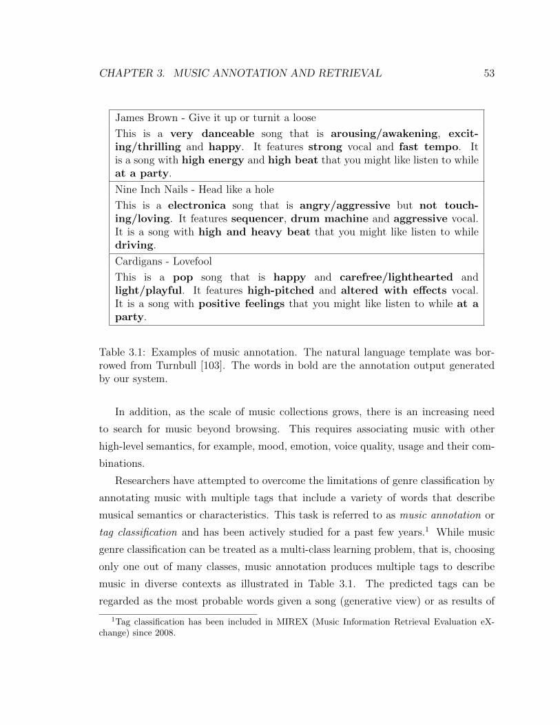
CHAPTER 3. MUSIC ANNOTATION AND RETRIEVAL 53
James Brown - Give it up or turnit a loose
This is a very danceable song that is arousing/awakening, excit-ing/thrilling and happy. It features strong vocal and fast tempo. Itis a song with high energy and high beat that you might like listen to whileat a party.
Nine Inch Nails - Head like a hole
This is a electronica song that is angry/aggressive but not touch-ing/loving. It features sequencer, drum machine and aggressive vocal.It is a song with high and heavy beat that you might like listen to whiledriving.
Cardigans - Lovefool
This is a pop song that is happy and carefree/lighthearted andlight/playful. It features high-pitched and altered with effects vocal.It is a song with positive feelings that you might like listen to while at aparty.
Table 3.1: Examples of music annotation. The natural language template was bor-rowed from Turnbull [103]. The words in bold are the annotation output generatedby our system.
In addition, as the scale of music collections grows, there is an increasing need
to search for music beyond browsing. This requires associating music with other
high-level semantics, for example, mood, emotion, voice quality, usage and their com-
binations.
Researchers have attempted to overcome the limitations of genre classification by
annotating music with multiple tags that include a variety of words that describe
musical semantics or characteristics. This task is referred to as music annotation or
tag classification and has been actively studied for a past few years.1 While music
genre classification can be treated as a multi-class learning problem, that is, choosing
only one out of many classes, music annotation produces multiple tags to describe
music in diverse contexts as illustrated in Table 3.1. The predicted tags can be
regarded as the most probable words given a song (generative view) or as results of
1Tag classification has been included in MIREX (Music Information Retrieval Evaluation eX-change) since 2008.

CHAPTER 3. MUSIC ANNOTATION AND RETRIEVAL 54
Query Top 5 Retrieved Songs
Angry/Aggressive (Emotion)
Nirvana - Aneurysm
Aphex Twin - Come to daddy
Rocket City Riot - Mine tonite
Metallica - One
Liz Phair - Supernova
Female Lead Vocals (Instrument)
Norah Jones - Don’t know why
Dido - Here with me
Sheryl Crow - I shall believe
No doubt - Simple kind of life
Carpenters - Rainy days and mondays
Alternatives (Genre)
Nirvana - Aneurysm
Oasis - Supersonic
Big Star - In the street
Gin Blossoms - Hey jealousy
Rocket City Riot - Mine tonite
Very Danceable (Usage)
LL Cool J - Mama said knock you out
2pac - Trapped
Jane’s addiction - Been caught stealing
Jackson 5 - Abc
Boogie Down Productions - The bridge is over
Table 3.2: Example of text-query based music retrieval. These are retrieval outputsgenerated by our system.
binary classification for the presence of each tag (discriminative view).
Meanwhile, annotation tasks usually produce a confidence score for each tag pre-
diction. For example, this confidence score can be a probability of a tag or a distance
from the decision boundary. This can be used to retrieve music using a text query
by sorting the confidence levels of the query word, i.e., the tags for each song in a
database. Therefore, music retrieval (query-by-text) can be performed as a byproduct
of the music annotation. Table 3.2 shows outcomes of the text-based music retrieval
for several descriptive words.

CHAPTER 3. MUSIC ANNOTATION AND RETRIEVAL 55
3.2 Previous Work
Music annotation is similar to genre classification in terms of the data processing
pipeline. Both of systems extract various audio features to characterize music at the
song level and then associate these features with labels. The main difference is that
genre classification is based on a winner-take-all scheme whereas music annotation
allows multiple labels to be selected. Thus, the majority of prior work in music
annotation has focused on multi-labeling algorithms while relying on popular audio
features from genre classification, for example, MFCC, dynamic MFCC and Auditory
Filterbank Temporal Envelope (AFTE).
One class of multi-labeling algorithms is based on fitting data to a generative
model that estimates a multinomial probability distribution for tags given a song.
This include a multi-class naıve Bayes approach [101], a Gaussian mixture model
using a weighted mixture hierarchies expectation-maximization (MixHier) [103] and
Codeword Bernoulli Average (CBA) model [38]. The MixHier model was progressively
improved by considering temporal dependency (Dynamic Texture Mixture) [18] or by
building up existing algorithms such as Decision Fusion [19]. These algorithms were
mainly evaluated on the CAL500 dataset that Turnbull et. al. released as a music
tagging dataset [102].
Another class of multi-labeling algorithms is based on a discriminative model that
finds a decision boundary of each tag using a binary classifier. This classification can
be implemented with SVM [100], AdaBoost [7] and logistic regression [26, 112]. It was
noted that these classifiers focus on binary classification accuracy rather than directly
optimizing the continuous confidence scores and thus the training can be suboptimal
for retrieval tasks [38]. However, recent results show that the distance from the
classifier’s decision boundary can be a reliable means to measure the confidence [26,
112].
While the previous work focused on multi-labeling algorithms, some researchers
were concerned with developing new audio features. In particular, they attempted to
discover audio features using learning algorithms instead of using features designed
with acoustic knowledge. However, most of the feature-learning approaches focused on

CHAPTER 3. MUSIC ANNOTATION AND RETRIEVAL 56
music genre classification as reviewed in the previous chapter whereas there have been
few attempts to apply the learning-based features to music annotation and retrieval.
Hamel and Eck developed DBN-based features for music classification and tagging
[32]. However, their experiment was not fully dedicated to annotation (i.e, tagging)
and retrieval. In addition, their sequel auto-tagging system focused on different types
of temporal pooling on a PCA-whitening domain rather than exploiting manifold
patterns of learned features [33].
In this chapter, we continue to evaluate our data processing pipeline in Chapter2
for music annotation and retrieval. However, leveraging the rich descriptions of tags
(rather than simply using genre), we will interpret the locally learned acoustic features
in more diverse musical semantics. In addition, we will extend the data processing
pipeline by applying DBNs to top of the song-level feature representation.
3.3 Proposed Method
3.3.1 Single Layer Model
We presented a feature-learning framework in Chapter 2. It constructs a song-level
feature in three steps. First, preprocessing is performed to normalize raw audio data
and return mel-frequency spectrogram. Second, high-dimensional sparse features are
locally learned on multiple frames of the mel-frequency spectrogram. Third, the local
feature vectors are max-pooled over a segment and the results are averaged over a
song. As a result, it produces a single high-dimensional vector for each song using an
unsupervised algorithm. For genre classification, we performed multi-class supervised
training with the feature vectors and genre labels using linear SVMs.
We apply this feature-learning framework to music annotation and retrieval as
well. In order to incorporate the framework into the multi-labeling problem, we
slightly modify the supervised training part. Previously, we adopted one-versus-all
scheme for multi-class classification. That is, we used one binary SVM for one genre
label so that only one label is set to 1 and all others to -1 for each song, as specified
in Equation 2.24. This can easily generalize to a multi-labeling problem simply by
CHAPTER 3. MUSIC ANNOTATION AND RETRIEVAL 57
setting more than one label to 1. For example, in genre classification, a typical label
vector y(i) is [1 -1 -1 -1 -1] or [-1 -1 1 -1 -1] where only one genre is selected among
five genres. In music annotation, we can set it to [1 -1 1 -1 -1] or [-1 1 1 -1 1]
where we set 1 when the corresponding tag is selected among five tags. In this way,
using the same objective function shown in Equation 2.24, we can concurrently train
multiple classifiers and perform multi-label classification. In addition, we can compute
distances from the decision boundary in a linear SVM (corresponding to a tag) to a
set of song-level features. They can be used as confidence levels for text-query based
music retrieval.
3.3.2 Extension to Deep Learning
A linear classifier has limitations in finding a complex decision boundary for a label in
the feature space, in our case, the presence of a tag in the song-level feature space. In
order to find a more accurate boundary, nonlinear classifiers using kernels or neural
networks are often chosen. In practice, the kernel approach, often an SVM with Radial
Basis function (RBF) or polynomial kernels, are preferred when building deep neural
networks because network performance is limited as the number of layers increases
[4].2 However, Hinton et. al. recently introduced a greedy layer-wise unsupervised
learning algorithm for the deep neural networks called Deep Belief Networks (DBN)
[36]. This has shown great promise as a strategy to train deep networks. Since then,
a great deal of research has been conducted in the area of neural networks. In Section
2.2, we briefly reviewed the DBN in feature-learning context. Here we apply the DBN
as a way of improving classifier performance.
The DBN is a generative model with many hidden layers. It is trained in an
unsupervised way by “greedy layer-wise stacking” of RBMs, which were introduced
in Section 2.3.3. First, a single layer RBM is trained to model the data. This RBM
learns a set of weights W and biases b, c in Equation 2.19. Then, we fix them as
the parameters of the first layer of the DBN. To learn the next layer of weights
2Deep neural networks are known to have poor training and generalization ability as the numberof hidden layers is greater than one or two. This is often attributed to gradient-based optimizationstarting from random initialization, which may get stuck near poor local optimum.

CHAPTER 3. MUSIC ANNOTATION AND RETRIEVAL 58
and biases, we compute the hidden layer representation discovered by the first layer
RBM using Equation 2.20 and apply these outputs as inputs to a new binary-binary
RBM (which has binary input units instead of Gaussian) to learn another layer of
the representation. This returns parameters for the next layer and deeper layers
are learned in a similar fashion. Hinton et. al. showed that the preceding learning
algorithm for a DBN always improves a variational lower bound on the log-likelihood
of the data when training more layers [36].
The DBN learns the most probable parameters to model the input data. The
parameters can be used to initialize deep neural networks instead of using random
initialization. This is often called “pre-training”. After this step, the deep network
can be trained with tags in a supervised way using back-propagation. This is often
called “fine-tuning” as a subsequent step to the pre-training. This approach for
learning deep networks has been shown to be essential for training deep networks.
We apply the DBN to model the song-level feature vectors. Figure 3.1 illustrates
a deep network built on top of our feature-learning framework to form a complete
system to estimate multiple tags. After we obtain the song-level features, we continue
to perform unsupervised learning by greedy layer-wise training up to the final hidden
layer and then fine-tune the network with tag labels using back-propagation. In
our experiment, we employed the L2-regularized L2 hinge-loss of the linear SVM in
Equation 2.24 with additional regularization terms of the network parameters as a
penalty function. This makes the penalty term consistent between classifiers. That
way, performance difference can be attributed only to the inclusion of the hidden
layer. Note that this architecture can be seen as a special case of a convolutional
deep network that connects a song (a long sequence of data) to a set of tags [50, 54].
However, the layers below and above the song-level feature have very different flavors.
Specifically, below the song-level feature, we focus on high-dimensional sparse feature
learning using a single layer on local data. Also, the layer remains unsupervised.
On the other hand, above the song-level feature, we perform dense feature learning
through multiple layers without sparsity and they are eventually supervised using the
tag information.

CHAPTER 3. MUSIC ANNOTATION AND RETRIEVAL 59
Tag 1 Tag 2 Tag 3 Tag 4
...
Mel!freq. Spectrogram
Seconds
Mel!f
req b
ins
0 0.5 1 1.5 2 2.5
20
40
60
80
100
120
Feature Bases
Hidden Layer Index
Mel!f
req b
ins
20
40
60
80
100
120
Hidden Layer Activation
Seconds
Hidd
en La
yer I
ndex
0 0.5 1 1.5 2 2.5
50
100
150
200
250
Song-Level Feature Vector
...
Mel!freq. Spectrogram
Seconds
Mel!
freq
bins
0 0.5 1 1.5 2 2.5
20
40
60
80
100
120
Feature Bases
Hidden Layer Index
Mel!
freq
bins
20
40
60
80
100
120
Hidden Layer Activation
Seconds
Hidd
en L
ayer
Inde
x
0 0.5 1 1.5 2 2.5
50
100
150
200
250
... ...
Local Sparse Features
Mel-Frequency Spectrogram
Max-Pooling / Aggregation
Feature Encoding
Hidden Layers
Figure 3.1: Feature-learning architecture using deep learning for multi-labeling clas-sification. A deep belief network is used on top of the song-level feature vectors andthen the network is fine-tuned with the tag labels.

CHAPTER 3. MUSIC ANNOTATION AND RETRIEVAL 60
3.4 Experiments
3.4.1 Datasets
We evaluated our multi-labeling system on CAL500, which is one of the most popular
datasets in music annotation and retrieval. CAL500 contains 502 western songs, each
of which was manually annotated with one or more tags out of 174 possibilities.
The tags are grouped into 6 categories: Mood, Genre, Instrument, Song, Usage, and
Vocal [102]. In our experiments, we used 97 tags with at least 30 example songs and
performed 5 fold cross-validation to compare results with those reported in previous
works. In order to apply the full path of our pipeline, we obtained MP3 files of the
502 songs and used the decoded waveforms.3
3.4.2 Preprocessing Parameters
We first resampled the waveform data to 22.05kHz and applied the time-frequency
AGC using 10 sub-bands and temporal smoothing the envelope on each band. We
computed an FFT with a 46ms Hann window and 50% overlap. This produces a 513
dimensional vector (up to half the sampling rate) for each frame. We then converted
it to a mel-frequency spectrogram with 128 bins. For the magnitude compression, C
was set to 10 (see Section 2.3.1).
3.4.3 MFCC
We also evaluated MFCC as a “hand-crafted” feature in order to compare it to
our proposed feature representation. Instead of using the MFCC provided from the
CAL500 dataset, we computed our own MFCC to match parameters as close as pos-
sible to the proposed feature. We used the same AGC and FFT parameters but 40
bins for the mel-frequency spectrogram and then applied log and DCT. In addition,
we formed a 39-dimensional feature vector by combining the delta and double delta
vector and normalized it by making the 39-dimensional vector have zero mean and
3Note that the decoded waveforms may be different from the original waveforms although theywill be perceptually very similar to each other.
CHAPTER 3. MUSIC ANNOTATION AND RETRIEVAL 61
unit variance. The MFCC vector was also fed into either the classifier directly or the
feature-learning step.
3.4.4 Feature-Learning Parameters
For the PCA whitening and feature-learning steps, we sampled 100000 data examples,
approximately 200 examples at random positions within each song 4. Each example
is selected as a 128 × n (n=1, 2, 4, 6, 8 and 10) patch from the mel-frequency
spectrogram. Using PCA whitening, we reduced the dimensionality of the examples
to retain 90% of the variance. Before the whitening, we added 0.01 to the variance
for regularization. We used dictionary size (or hidden layer size) and sparsity (when
applicable) as the primary feature-learning meta parameters. The dictionary size was
fixed to 1024. The sparsity parameter was set to ρ = 0.007, 0.01, 0.02, 0.03, 0.05, 0.07
and 0.1 for sparse RBM and λ = 1.0, 1.5, 2.0 and 2.5 for sparse coding. Max-pooling
was performed over segments of length 0.05, 0.1, 0.25, 0.5, 1, 2, 4, 8, 16, 32 and 64
seconds. Note that we performed the PCA whitening and feature learning only with
a training set, that is, separately for each fold of cross validation.
3.4.5 Classifier Parameters
We first normalized the song-level features of the training set by subtracting the mean
and dividing by the standard deviation. We then trained the classifiers with the
features and hard annotation. All parameters in preprocessing and feature-learning
stages were tuned using linear SVMs. Using the best parameter set, we replaced the
single-layer classifier with deep neural networks with up to three hidden layers. In
order to verify the effectiveness of the DBN, we compared the pre-training by DBN
with random initialization for the deep neural networks. In the deep neural network,
all hidden layer sizes were fixed to 512 units. Finally, to suppress frequently used tags
and thus makes more balanced predictions, we adjusted the distance to the decision
4In our previous work, we sampled examples only once from the whole dataset. In this experiment,we sampled them from the training set and learned parameters separately for each fold. Thus, theresults are slightly different from those in [71].

CHAPTER 3. MUSIC ANNOTATION AND RETRIEVAL 62
boundary by subtracting the mean times diversity factor (1.25) from the classifier
output, following the heuristic in [38].
3.5 Evaluation and Discussion
3.5.1 Visualization
Figure 3.2 shows feature bases learned from the CAL500 dataset using a sparse RBM.
Using the procedure in Section 2.5.1, given a tag label we searched 20 most active
feature bases and organized them for each group of tags. As previously shown with
the genre dataset, they are distinguished by different timbral patterns. In particular,
by virtue of the rich words of musical semantics in the dataset, the results effectively
demonstrate that the semantic descriptions are associated with the local acoustics
patterns.Table 3.3 summarizes the relationships for selected tags. It suggests that
songs with a specific tag activate certain feature bases more frequently. This demon-
strates that the feature bases are selectively activated depending on the semantics of
music, thereby helping discriminate music at the high-level.
3.5.2 Evaluation Metrics
We evaluated the annotation task using precision, recall and F-score, following pre-
vious work. Precision and recall were computed based on the methods described by
Turnbull [103]. The F-score was computed by first calculating individual F-scores for
each tag and then averaging the individual F-scores, similarly to what was done by
Ellis [26]. It should be noted that averaging individual F-scores tends to generate
lower average F-score than computing the F-score from mean precision and recall val-
ues. As for the retrieval, we used the area under the receiver operating characteristic
curve (AROC), mean average precision (MAP) and top-10 precision (P10) [26].

CHAPTER 3. MUSIC ANNOTATION AND RETRIEVAL 63
Angry/Agressive
Mel−
frequency
bin
20
40
60
80
100
120
Calming/Soothing
20
40
60
80
100
120
Exciting/Thrilling
20
40
60
80
100
120
Happy
20
40
60
80
100
120
Sad
20
40
60
80
100
120
(a) Emotion
Aggressive
Mel−
frequency
bin
20
40
60
80
100
120
High−pitched
20
40
60
80
100
120
Low−pitched
20
40
60
80
100
120
Rapping
20
40
60
80
100
120
Screaming
20
40
60
80
100
120
(b) Vocal
ElectricGuitar(distorted)
20
40
60
80
100
120
DrumMachine
20
40
60
80
100
120
FemaleLeadVocals−Solo
20
40
60
80
100
120
MaleLeadVocals−Solo
20
40
60
80
100
120
Trumpet
20
40
60
80
100
120
(c) Instrument
Driving
Me
l−fr
eq
ue
ncy b
in
20
40
60
80
100
120
Reading
20
40
60
80
100
120
Romancing
20
40
60
80
100
120
Sleeping
20
40
60
80
100
120
Wakingup
20
40
60
80
100
120
(d) Usage
Figure 3.2: Top 20 most active feature bases (dictionary elements) learned by a sparseRBM for different emotions, vocal quality, instruments and usage categories of theCAL500 set.

CHAPTER 3. MUSIC ANNOTATION AND RETRIEVAL 64
Tag Description on feature bases
Angry/Aggressive Wideband energy with strong high-frequencycontent or extreme low-frequency content
Calm/Soothing and Sleeping Low-frequency content with harmonic patterns
Low-pitched and High-pitched Juxtaposed with low- and high-pitched harmonicpatterns
Rapping and DrumMachine Extremely low-freq. energy and several wide-band and transient patterns
Exciting/Thrilling Non-harmonic and transient patterns
Table 3.3: This table describes the acoustic patterns of the feature bases that areactively “triggered” in songs with a given tag. The corresponding feature bases areshown in Figure 3.2.
3.5.3 Results and Discussion
We examine the effect of preprocessing and feature-learning algorithms on the anno-
tation and retrieval performance. Also, we show improved results with deep neural
networks. Finally, we compare our best results to those of state-of-the-art algorithms.
Input Data, Algorithms and AGC
Table 3.4 summarizes results on features obtained with different types of input data
and feature-learning algorithms. First of all, the mel-frequency spectrogram signifi-
cantly outperforms MFCC regardless of the type of learning algorithms. This indi-
cates that capturing rich acoustic patterns (not just timbre with MFCC but also pitch
and harmony) from mel-frequency spectrogram is necessary to effectively associate
sound with musical semantics. Among the feature-learning algorithms, K-means and
sparse RBM generally perform better than sparse coding, which is somewhat dif-
ferent from the genre classification result in the previous chapter. In addition, the
results show that the time-frequency AGC significantly improves both annotation and

CHAPTER 3. MUSIC ANNOTATION AND RETRIEVAL 65
Annotation Retrieval
Data+Algorithm Prec. Recall F-score AROC MAP P10
With AGC
MFCC only 0.399 0.223 0.242 0.713 0.446 0.467
MFCC+K-means 0.446 0.240 0.270 0.732 0.471 0.492
MFCC+SC 0.437 0.232 0.260 0.713 0.452 0.476
MFCC+SRBM 0.441 0.235 0.263 0.725 0.463 0.485
Mel-Spec+K-means 0.467 0.253 0.289 0.740 0.487 0.515
Mel-Spec+SC 0.458 0.250 0.283 0.733 0.481 0.509
Mel-Spec+SRBM 0.474 0.258 0.290 0.741 0.489 0.513
Without AGC
MFCC only 0.399 0.222 0.239 0.712 0.444 0.460
MFCC+K-means 0.438 0.237 0.267 0.727 0.465 0.489
Mel-Spec+SRBM 0.458 0.246 0.275 0.727 0.478 0.506
Table 3.4: Performance comparison for different input data and feature-learning al-gorithms. These results are all based on linear SVMs.
retrieval performance, regardless of the input features.
Receptive Field Size
Figure 3.3 plots F-score and AROC for different receptive field size, that is, the
number of frames taken from the mel-frequency spectrogram. It shows that the
performance significantly increases between 1 and 4 frames and then saturates beyond
4 frames. It is interesting that the best results are achieved at 6 frames (about
0.16 second long). We think this is related to the representational power of the
algorithm. That is, when the number of frames is small, the algorithm is capable of
capturing the variation of input data. However, as the number of frames grows, the
algorithm becomes incapable of representing the exponentially increasing variation,
in particular, temporal variation.

CHAPTER 3. MUSIC ANNOTATION AND RETRIEVAL 66
1 2 4 6 8 100.26
0.265
0.27
0.275
0.28
0.285
0.29
0.295
Number of frames
F−
sco
re
SC
RBM
Kmeans
(a) F-score
1 2 4 6 8 100.71
0.715
0.72
0.725
0.73
0.735
0.74
0.745
0.75
Number of frames
AR
OC
SC
RBM
Kmeans
(b) AROC
Figure 3.3: Effect of number of frames. The dictionary size is set to 1024.
Sparsity and max-pooling size
Figure 3.5 plots the F-score for a set of sparsity values and max-pooling sizes. It shows
a clear trend that higher accuracy is achieved when the feature vectors are sparse
(around 0.02) and max-pooled over segments of about 16 seconds.5 These results
indicate that the best discriminative power in song-level classification is achieved by
capturing only a few important features over both timbral and temporal domains.
Deep Learning
Table 3.5 shows results when deep neural networks are used. The preprocessing
and feature-learning parameters were chosen from the best result with linear SVMs.
In general, pre-training outperforms random initialization regardless of the number
of hidden layers. With random initialization, the best result was obtained with a
single hidden layer (Mel-SRBM-NN1) and, as more hidden layers are used, the result
became worse. This is probably because it becomes more difficult to find a good
5We found that the average length of songs on the CAL500 dataset is approximately 250 seconds,which suggests that aggregating about 16 (≈ 250/16) max-pooled feature vectors over an entire songis an optimal choice.

CHAPTER 3. MUSIC ANNOTATION AND RETRIEVAL 67
0.007 0.01 0.02 0.03 0.05 0.07 0.10.28
0.282
0.284
0.286
0.288
0.29
Sparsity
F−
sco
re
(a) F-score
0.007 0.01 0.02 0.03 0.05 0.07 0.10.732
0.734
0.736
0.738
0.74
0.742
0.744
SparsityA
RO
C
(b) AROC
Figure 3.4: Effect of sparsity (sparse RBM).
0.1 0.25 0.5 1 2 4 8 16 32 640.265
0.27
0.275
0.28
0.285
0.29
Max−pooling [sec]
F−
sco
re
(a) F-score
0.1 0.25 0.5 1 2 4 8 16 32 640.728
0.73
0.732
0.734
0.736
0.738
0.74
0.742
0.744
Max−pooling [sec]
AR
OC
(b) AROC
Figure 3.5: Max-pooling of sparsity (sparse RBM).

CHAPTER 3. MUSIC ANNOTATION AND RETRIEVAL 68
Annotation Retrieval
Classifiers Prec. Recall F-score AROC MAP P10
Linear SVM
Mel-SRBM-SVM 0.479 0.257 0.289 0.741 0.489 0.513
Neural networks with hinge loss (random initialization)
Mel-SRBM-NN1 0.470 0.256 0.291 0.756 0.505 0.531
Mel-SRBM-NN2 0.481 0.244 0.285 0.749 0.498 0.531
Mel-SRBM-NN3 0.467 0.236 0.280 0.728 0.479 0.500
Neural networks with hinge loss (pre-trained by DBNs)
Mel-SRBM-DBN1 0.488 0.260 0.295 0.757 0.508 0.532
Mel-SRBM-DBN2 0.476 0.256 0.291 0.754 0.509 0.546
Mel-SRBM-DBN3 0.476 0.253 0.286 0.752 0.507 0.531
Table 3.5: Performance comparison for linear SVM and neural networks with randominitialization (Mel-SRBM-NN*) and pre-training by DBN (Mel-SRBM-DBN*). Thefigures (1, 2 and 3) indicate the number of hidden layers. The receptive field size wasset to 6 frames.
local optimum as the number of parameter increases. With pre-training by DBN, the
best result was obtained with one and two hidden layers (Mel-SRBM-DBN1 and Mel-
SRBM-DBN2). They achieved the highest accuracy in both annotation and retrieval.
These results show that the DBN is an effective strategy for training a deep neural
network as a classifier.
Comparison to state-of-the-art algorithms
Table 3.6 compares our best results to those of state-of-the-art algorithms from the
group that developed CAL500. The group used MFCC features as input data and
modeled the features using either Gaussian Mixture Model (GMM) as a bag of frames
[103] or Dynamic Texture Mixture (DTM) considering temporal dependency [18].
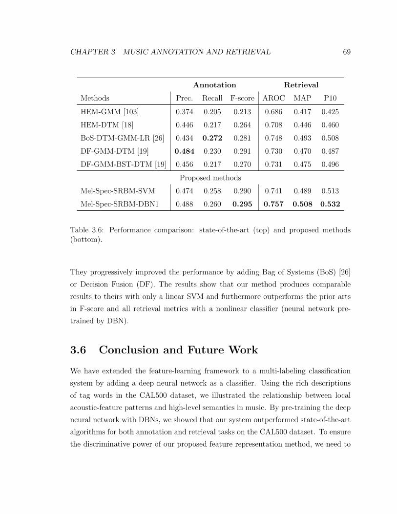
CHAPTER 3. MUSIC ANNOTATION AND RETRIEVAL 69
Annotation Retrieval
Methods Prec. Recall F-score AROC MAP P10
HEM-GMM [103] 0.374 0.205 0.213 0.686 0.417 0.425
HEM-DTM [18] 0.446 0.217 0.264 0.708 0.446 0.460
BoS-DTM-GMM-LR [26] 0.434 0.272 0.281 0.748 0.493 0.508
DF-GMM-DTM [19] 0.484 0.230 0.291 0.730 0.470 0.487
DF-GMM-BST-DTM [19] 0.456 0.217 0.270 0.731 0.475 0.496
Proposed methods
Mel-Spec-SRBM-SVM 0.474 0.258 0.290 0.741 0.489 0.513
Mel-Spec-SRBM-DBN1 0.488 0.260 0.295 0.757 0.508 0.532
Table 3.6: Performance comparison: state-of-the-art (top) and proposed methods(bottom).
They progressively improved the performance by adding Bag of Systems (BoS) [26]
or Decision Fusion (DF). The results show that our method produces comparable
results to theirs with only a linear SVM and furthermore outperforms the prior arts
in F-score and all retrieval metrics with a nonlinear classifier (neural network pre-
trained by DBN).
3.6 Conclusion and Future Work
We have extended the feature-learning framework to a multi-labeling classification
system by adding a deep neural network as a classifier. Using the rich descriptions
of tag words in the CAL500 dataset, we illustrated the relationship between local
acoustic-feature patterns and high-level semantics in music. By pre-training the deep
neural network with DBNs, we showed that our system outperformed state-of-the-art
algorithms for both annotation and retrieval tasks on the CAL500 dataset. To ensure
the discriminative power of our proposed feature representation method, we need to

CHAPTER 3. MUSIC ANNOTATION AND RETRIEVAL 70
evaluate it on larger datasets, such as, the Million Song Dataset [8] or Magnatagatune
[49].

Chapter 4
Piano Transcription Using Deep
Learning
4.1 Introduction
Music transcription is the task of inferring a symbolic representation (e.g., musical
notes) from audio recordings. Musical notes are often played simultaneously and
thus individual notes interfere with each other by virtue of their harmonic relations.
In addition, timbre, tuning and room conditions vary all the time. The polyphonic
nature of music and the acoustic variations make music transcription a challenging
problem.
A number of methods have been proposed since Moorer first attempted to use
computers to transcribe two voices of different musical instruments [68]. State-of-
the-art algorithms can be divided into three categories: iterative F0 searches, joint
source estimation and classification-based methods. Iterative F0-searches first find
the predominant F0 and then subtract its relevant sources (e.g., harmonic partials)
from the input signal. They repeat this procedure on what remains until no additional
F0s are found [48]. Joint source estimation examines possible combinations of sound
sources by hypothesizing that the input signal is approximated by a weighted sum of
the sound sources with different F0s [31, 95].
While these two categories are based on a generative approach that find a group of
71

CHAPTER 4. PIANO TRANSCRIPTION USING DEEP LEARNING 72
Waveforms Feature Representations
Binary Classifier
Binary Classifier
Binary Classifier. . .
. . .
C4# note on/off
C4 note on/off
B3 note on/off
Figure 4.1: Classification-based polyphonic note transcription. Each binary classifierdetects the presence of a note.
notes that constitute an observed polyphonic tone, classification-based methods are
based on a discriminative approach which detects the presence of a note from the poly-
phonic tone. They usually use multiple binary classifiers, each of which are trained
with short-time acoustic features and single note labels (i.e., note on/off). They
collectively detect multiple notes simultaneously as shown in Figure 4.1. Although
classification-based methods typically make relatively less use of acoustic knowledge,
they showed comparable results to iterative F0 searches and joint source estimation,
particularly for piano music [64, 85].
However, there are two main issues to address in the classification-based methods.
First, the discriminative approach usually requires a large dataset to generalize well
[75]. This requires good feature representations invariant to diverse variations in the
large dataset. Second, each classifier is usually trained separately for each note. This
can be computationally expensive especially when the dimensionality of features is
high or the classifiers have many meta parameters that require cross-validation.
In this chapter, we present a new classification-based algorithm for polyphonic
piano note transcription that considers these two issues. Specifically, we extend a
previous classification-based method in two ways: (1) by using feature representations
learned from spectrogram data and (2) by jointly training the classifiers for multiple
notes. We obtain the learned features using deep belief networks and, in turn, use the
network to concurrently train multiple binary classifiers. We evaluate our approach on

CHAPTER 4. PIANO TRANSCRIPTION USING DEEP LEARNING 73
several public piano transcription datasets and show that our approach outperforms
compared music transcription methods 1.
4.2 Previous Work
The discriminative approach is based on finding an optimal boundary for the presence
of each note by supervised learning. A single note has variations due to timbre, tuning,
room acoustics (e.g., reverberation or background noise) and mixing with other notes.
Previous work has attempted to find the complex boundary by developing robust
features to the acoustic variations and feeding them into sophisticated classifiers,
mainly focusing on polyphonic piano transcription.
Marolt used an auditory filter model and adaptive oscillator networks as a front-
end processing [64]. The auditory filter model emulates the functionality of human
ear producing quasi-periodic firing activities of inner hair cells on a set of frequency
channels and the adaptive oscillator networks track partials and group harmonically
related ones. He used the output of the oscillator network module as a note-detection
feature and applied it to neural networks for supervised training. Poliner and Ellis
proposed a simpler discriminative model. They used a normalized spectrogram as
a timbre-invariant feature and applied it to support vector machine (SVM) with an
RBF kernel [85]. Then, they temporally smoothed the resulting prediction of the
note presence using Hidden Markov Models (HMMs). Boogaart and Lienhart used
a similar approach. They adopted multiple frames of Gabor transform as an input
feature and Adaboost as a note classifier, instead [106].
These methods in common used novel features and non-linear classifiers to find
the complex boundary of note presence. The features were designed by using different
time-frequency transforms and refining them in a hand-tuned manner. In addition,
they sampled positive and negative examples separately for each binary note classifier
and trained them independently. Since the majority of pianos have 88 notes, this
training strategy can be computationally expensive especially when the feature is
high-dimensional or classifiers have many meta parameters.
1This chapter is based on our previous work [72].

CHAPTER 4. PIANO TRANSCRIPTION USING DEEP LEARNING 74
There is increasing interest in learning the feature from data using unsupervised
learning algorithms as an alternative to the hand-tuning approach. Researchers dis-
covered that the learning algorithms can find the underlying structure of data and
provide the outcome as a new feature representation. Furthermore, this adaptively
learned feature was shown to be highly effective in a number of classification tasks.
We apply this feature-learning approach to classification-based polyphonic piano tran-
scription. We will show that this approach is highly effective with only a linear
classifier. Also, we propose a strategy to efficiently train note classifiers.
4.3 Proposed Method
4.3.1 Feature Representation By Deep Learning
A restricted Boltzmann machine (RBM) is an unsupervised learning algorithm that
has two layers: a visible layer and a hidden layer. The visible layer corresponds to
the input data while the hidden layer represents features discovered by training the
RBM. In Chapter 2 and 3, we used a sparse version of RBM where the binary units of
the hidden layer are constrained to be parsimoniously activated. We showed that the
sparse RBM captures acoustic patterns that explain musical signals and the outcome
was used as a novel feature representation for music classification.
We apply the sparse RBM to piano sounds in order to discover their harmonic
patterns and use them for classification-based polyphonic piano transcription. Specif-
ically, we model single frames of normalized spectrogram with the sparse RBM; the
visible layer corresponds to a vector of the spectrogram frame. Figure 4.2 illustrates
the feature bases learned from a large piano dataset using the sparse RBM. Most bases
capture harmonic distributions, which correspond to various pitches while some con-
tain non-harmonic patterns. Also, note that the feature bases show exponentially
growing curves for each harmonic partial. This verifies the structure of the piano
sound, i.e., the logarithmic scale of musical notes.
On top of the first RBM, we stack another RBM to find more complex dependency
in piano sounds, for example, different combinations of the features shown in Figure

CHAPTER 4. PIANO TRANSCRIPTION USING DEEP LEARNING 75
Figure 4.2: Feature bases learned from a piano dataset using a sparse RBM. Theywere sorted by the frequency of the highest peak. Most bases capture harmonicdistributions which correspond to various pitches while some contain non-harmonicpatterns. Note that the feature bases show exponentially growing curves for eachharmonic partial. This verifies the logarithmic scale in the piano sound.
4.2. This is performed by greedy layer-wise training, that is, using the feature data
from the first RBM to train another RBM. This deep learning algorithm is called a
deep belief network (DBN) [36]. In Chapter 3, we used DBNs as a means to achieve
“better initialization” for neural networks in the context of supervised training. Thus
we compared it to randomly initialized neural networks. Here we intend to use them as
a multi-layer feature-learner. Thus, we first examine the DBN output (the top hidden
layer of the pre-trained network) as a feature representation for note classifiers. Then,
we will fine-tune the network by back-propagating the errors from the classifiers. In
our experiments, we evaluated up to two layers of DBNs and compared the pre-trained
network to the fine-tuned one.

CHAPTER 4. PIANO TRANSCRIPTION USING DEEP LEARNING 76
4.3.2 Training Strategy
A piano usually has 88 notes, each of which is detected by the corresponding binary
classifier. They can be trained either separately for each note or jointly as a multi-
labeling problem. We term the two training strategies as single-note training and
multiple-note training, respectively, and describe them below.
Single-note Training
The majority of previous classification-based methods trained classifiers individually
for each note. For example, Poliner and Ellis’ piano transcription system consists
of 87 independent support vector machine (SVM) classifiers with an RBF kernel.
They formed the training data by selecting spectrogram frames that include the note
(positive examples) and those that do not include it (negative examples). They
randomly sampled 50 positive (when available) and negative examples from each
piano song per note and trained the SVM with separate training data for each note.
We also examine this single-note training strategy. However, instead of a nor-
malized spectrogram along each frequency axis that they used, we apply DBN-based
feature representations of spectrogram frames. In addition, we constrained the SVM
to a linear kernel because they reported that the RBF kernel provided only modest
performance gains with significantly more computation [86] and also a linear SVM
is more suitable to large-scale data. The left column of Figure 4.3 illustrates our
approach for single-note training. Our proposed method transforms the spectrogram
frames into mid-level features via one or two layers of learned networks and then feeds
them into the classifier. As an additional step, we fine-tune the network using the
error from the linear SVM. We compare this with a baseline model that directly feed
spectrogram frames into the SVM.
Multiple-note Training
While examining the single-note training, we observed that the trained classifiers tend
to be somewhat “aggressive”. In other words, they produced more “false alarm” errors
(detection of inactive notes as active ones) than “miss” errors (failure to detect active

CHAPTER 4. PIANO TRANSCRIPTION USING DEEP LEARNING 77
notes). In particular, this significantly degraded onset accuracy. Also, the training
was slow because the deep networks had to be fine-tuned separately for each note.
For this reason, we attempted to train all binary classifiers concurrently, referring to
this as multiple-note training.
The idea is that we can view the polyphonic piano transcription as a multi-labeling
problem, that is, labeling 88 binary note-on/off tags given an audio feature. We have
already handled this problem for music annotation in Chapter 3, where we performed
the training by summing multiple SVM objectives using shared features and the
binary label vectors.2 This allows cross-validation to be jointly performed for the
combined SVMs, thereby saving a significant amount of training time. On the other
hand, this requires a different way of sampling examples because the training data is
shared by all binary classifiers. Since we combined all 88 notes in our experiments, all
spectrogram frames except silent ones are a positive example for at least one SVM.
Thus we sampled the training data by simply selecting every K spectrogram frame.
K was set to 16 as a trade-off between data reduction and performance. Note that
this makes the ratio of positive and negative examples for each SVM determined
by occurrences of the note in the whole training set, thereby having significantly
more negative examples than positive ones for most SVMs. It turned out that this
“unbalanced” data ratio makes the classifiers “less aggressive,” as a result, increasing
overall performance.
The right column of Figure 4.3 illustrates the multiple-note training. Before the
fine-tuning, the binary classifiers, in fact, do not influence each other. However, when
the fine-tuning is performed, the errors of the classifiers collaboratively update the
shared network. In other words, the presence of multiple notes such as C3 or C4
jointly updates the learned features, improving the overall performance.
4.3.3 HMM Post-processing
The note on/off classification described above treats training examples independently
without considering dependency between neighboring frames. We temporally smooth
2This approach is described as a multi-labeling problem in Section 3.3.1. The objective functionis denoted in Equation 2.24.

CHAPTER 4. PIANO TRANSCRIPTION USING DEEP LEARNING 78
...
... Input
Multiple-NoteTraining
Linear SVM
(Baseline)
Linear SVM
+ Hidden Layers
...
Single-NoteTraining
Output
...
...
...
...
...
...
Output
Input
HiddenLayers
...
Figure 4.3: Network configurations for single-note and multiple-note training. Fea-tures are obtained from feed-forward transformation as indicated by the bottom-uparrows. They can be fine-tuned by back-propagation as indicated by the top-downarrows.

CHAPTER 4. PIANO TRANSCRIPTION USING DEEP LEARNING 79
the output of classifiers using HMM-based post-processing, following Poliner and Ellis.
We model each note independently with a two-state HMM and modified the SVM
output (distance to the decision boundary) to obtain a posterior probability:
p(yi = 1|xi) = sigmoid(α(θTxi)), (4.1)
where xi is a feature vector, θ are SVM parameters, yi is a label and α is a scaling
constant. α was chosen from a pre-determined list of values as part of the cross-
validation stage. For each note class, the smoothing process was performed by running
a Viterbi search based on a 2x2 transition matrix, a note on/off prior (for obtained
from the training data) and the posterior probability.3
Figure 4.4 shows the overall signal transformation through the DBN networks,
SVM classifiers and HMM post-processing. Note that the original spectrogram grad-
ually changes, getting more similar to the final output.
4.4 Experiments
4.4.1 Datasets
We used three publicly available piano datasets to evaluate our approach.
Poliner and Ellis
This data set consists of 124 MIDI files of classical piano music. They were rendered
into 124 synthetic piano sound and 29 real piano recordings [85]. We used the first
60-second excerpt of each song.
MAPS
MIDI-Aligned Piano Sounds (MAPS) is a large piano dataset that includes various
patterns of playing and pieces of music [27]. We used 9 sets of piano pieces, each with
3We used HMMTool box found at http://www.cs.ubc.ca/~murphyk/Software/HMM/hmm.html

CHAPTER 4. PIANO TRANSCRIPTION USING DEEP LEARNING 80
Input (Spectrogram ) Hidden layer activation
HMM outputSVM output
Time (10ms)
Freq
uenc
y [k
Hz]
100 200 300 4000
0.5
1
1.5
Time (10ms)H
idde
n un
it in
dex
100 200 300 400
50
100
150
200
250
Time (10ms)
MID
I not
e nu
mbe
r
100 200 300 400
40
60
80
100
Time (10ms)
MID
I not
e nu
mbe
r
100 200 300 400
40
60
80
100
Figure 4.4: Signal transformation through our system. The original spectrogramgradually changes to the final output via the deep network, SVM classifiers andHMM-based smoothing
CHAPTER 4. PIANO TRANSCRIPTION USING DEEP LEARNING 81
30 songs. They were created by various high-quality software synthesizers (7 sets)
and Yamaha Disklavier (2 sets). We used the first 30-second excerpt of each song in
the validation and test sets but the same length at a random position for the training
set.
Marolt
Marolt provided a small number of piano examples that consists of 3 synthetic piano
and 3 real piano recordings [64]. This small dataset was used only in the testing
phase.
4.4.2 Pre-processing
We first computed spectrograms from the datasets with a 128ms window and 10ms
overlaps. To remove note dynamics, we normalized each column by dividing entries
by their sum, and then compressed it using a cube root, commonly used as an ap-
proximation to the loudness sensitivity of human ears. Furthermore, we applied PCA
whitening to the normalized spectrogram, retaining 99% of the training data variance
and adding 0.01 to the variance before the whitening. This yielded roughly 50-60%
dimensionality reduction and lowpass filtering in the PCA domain. The ground truth
was created from the MIDI files. We extended note offset times by 100ms in all train-
ing data to account for room reverberation in the piano recordings. The extended
note length was experimentally determined.
4.4.3 Unsupervised Feature Learning
We trained the first and second-layer DBN representations using the pre-processed
spectrogram. The hidden layer size was chosen as 256 and the expected activation
of hidden units (sparsity) was cross-validated over 0.05, 0.1, 0.2 and 0.3, while other
parameters were kept fixed.
CHAPTER 4. PIANO TRANSCRIPTION USING DEEP LEARNING 82
4.4.4 Evaluation Metrics
We primarily used the following metric of accuracy:
Accuracy =TP
FP+FN+TP, (4.2)
where TP (true positive) is the number of correctly predicted examples, FP (false pos-
itives) is the number of note-off examples transcribed as note-on, FN (false negative)
is the number of note-on examples transcribed as note-off. This metric is used for
both frame-level and onset accuracy. Frame-level accuracy is measured by counting
the correctness of frames every 10ms, and onset accuracy is by searching a note onset
of the correct pitch within 100 ms of the ground-truth onset. In addition, we used the
F-measure for frame-level accuracy to compare our results to those published using
the metric.
4.4.5 Training Scenarios
Our method is evaluated in two different scenarios. In the first scenario, we primarily
used the Poliner and Ellis set, splitting it into training, validation and test data fol-
lowing [85]. In order to avoid overfitting to the specific piano set, we selected 26 songs
from two synthesizer pianos sets in MAPS and used them as an additional validation
set. For convenience, we refer to this subset as MAPS2. In the second scenario, we
used five remaining synthesizer piano sets in MAPS for training to examine if our
method generalizes well when trained on diverse types of timbre and recording condi-
tions. For validation, we randomly took out 26 songs from the five piano sets, calling
them MAPS5 to distinguish it from the actual training data. We additionally used
MAPS2 for validation in the second scenario as well.4
4The lists of MAPS songs for training, validation and test are specified in http://ccrma.
stanford.edu/~juhan/ismir2011.html

CHAPTER 4. PIANO TRANSCRIPTION USING DEEP LEARNING 83
4.5 Evaluation
4.5.1 Validation Results
We compare the baseline feature (normalized spectrogram by cube root) to the first-
and second-layer DBN features and their fine-tuned versions on validation sets in the
two scenarios. The results are shown in Figure 4.5 and 4.6.
In scenario 1, DBN features generally outperform the baseline. In single-note
training, fine-tuned L1-features give the highest accuracy on both validation sets. In
multiple-note training, unsupervised L1- or L2-features achieve slightly better results.
In a comparison of the two training methods, either one appears to be not superior
to the other, showing subtle differences: Multiple-note training gives slightly better
results when the same piano set are used for validation (Poliner and Ellis), whereas
single-note training does a little better job when different pianos set (MAPS2) are
used.
In scenario 2, the results show that DBN L1-features always achieve better results
than the baseline but DBN L2-features generally give worse accuracy. Fine-tuning
always improves results on both validation sets, although the increment is very lim-
ited on MAPS2 in multiple-note training. In comparison of the two training methods,
multiple-note training outperforms single-note training for both validation sets, par-
ticularly giving the best accuracy on MAPS2. The superiority of multiple-note train-
ing is even more apparent in onset accuracy as shown in Figure 4.6. This is because
the multiple-note training is less aggressive and therefore it has less false alarms.
Figure 4.7 shows the influence of sparsity (hidden layer activation in RBMs)
on frame-level accuracy. The accuracy is the average value on two validation sets
(MAPS5 and MAPS2) when L1 features are used in multiple-note training and sce-
nario 2. The results indicate that relatively less sparse features perform better before
fine-tuning; however, with fine-tuning, sparse features achieve the highest accuracy
as well as the best improvement.

CHAPTER 4. PIANO TRANSCRIPTION USING DEEP LEARNING 84
40
50
60
70
80
90
Acc
urac
y (%
)
Single−note training Multiple−note training
Poliner Ellis
MAPS2
Poliner Ellis
MAPS2
Baseline
L1
L1−finetuned
L2
L2−finetuned
(a) Scenario 1
40
50
60
70
80
90
Acc
urac
y (%
)
Single−note training Multiple−note training
MAPS5
MAPS2
MAPS5
MAPS2
(b) Scenario 2
Figure 4.5: Frame-level accuracy on validation sets in two scenarios. The first andsecond-layer DBN features are referred to as L1 and L2.
4.5.2 Test Results: Comparison With Other Methods
The validation results show that a single layer of DBN is the best-performing feature
representation and multiple-note training is better than single-note training. Thus, we
chose DBN L1-features and multiple-training to test our system. Also, we evaluated
both unsupervised and fine-tuned features.
Table 4.1 shows results on the Poliner and Ellis test set, and Marolt set. We
divided the table into two groups to make a fair comparison. The upper group uses
the same dataset for both training and testing (the Poliner and Ellis set) whereas
the lower group assumes that the piano tones in the test sets were “unheard” in
training or uses different transcription algorithms. In the upper group, Poliner and
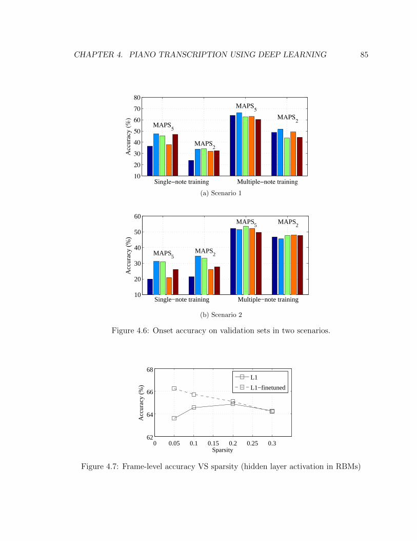
CHAPTER 4. PIANO TRANSCRIPTION USING DEEP LEARNING 85
10
20
30
40
50
60
70
80
Acc
urac
y (%
)
Single note training Multiple note training
MAPS5
MAPS2
MAPS5MAPS2
(a) Scenario 1
10
20
30
40
50
60
Acc
urac
y (%
)
Single−note training Multiple−note training
MAPS5
MAPS2
MAPS5
MAPS2
(b) Scenario 2
Figure 4.6: Onset accuracy on validation sets in two scenarios.
0 0.05 0.1 0.15 0.2 0.25 0.362
64
66
68
Sparsity
Acc
urac
y (%
)
L1
L1−finetuned
Figure 4.7: Frame-level accuracy VS sparsity (hidden layer activation in RBMs)

CHAPTER 4. PIANO TRANSCRIPTION USING DEEP LEARNING 86
Algorithms P. and E. Marolt
Poliner and Ellis [85] † 67.7% 44.6%
Proposed (S1-L1) 71.5% 47.2%
Proposed (S1-L1-fine-tuned) 72.5% 46.45%
Marolt [64] † 39.6% 46.4%
Ryyananen and Klapuri [87] † 46.3% 50.4%
Proposed (S2-L1) 63.8% 52.0%
Proposed (S2-L1-fine-tuned) 62.5% 51.4%
Table 4.1: Frame-level accuracy on the Poliner and Ellis, and Marolt test set. Theupper group was trained with the Poliner and Ellis train set while the lower groupwas with other piano recordings or uses different methods. S1 and S2 refer to trainingscenarios. †These results are from Poliner and Ellis [85].
Ellis’ transcription system adopted a normalized spectrogram and a non-linear SVM.
Our method outperformed their approach for both test sets. In the lower group, our
method trained with MAPS (scenario 2) also produced better accuracy than the two
published results on both sets. Note that, in both groups, unsupervised features give
better results than fine-tuned features when different piano sets are used for training
and testing. As for onset accuracy, we achieved 62% in training scenario 1 on the
Poliner and Ellis test set, which is very close to the Poliner and Ellis’ result (62.3%).
Table 4.2 compares our method with other algorithms evaluated on the MAPS
test set, composed of 50 songs selected from the two Disklavier piano sets by [107].
The fine-tuned DBN-features in our method give the highest frame-level accuracy
among compared methods.
4.6 Discussion and Conclusions
We have applied DBNs to classification-based polyphonic piano transcription. The
results show that learned feature representations by DBNs, particularly L1 features,

CHAPTER 4. PIANO TRANSCRIPTION USING DEEP LEARNING 87
Algorithms Precision Recall F-measure
Marolt [64] † 74.5% 57.6% 63.6%
Vincent et al. [107] † 71.6% 65.5% 67.0%
Proposed (S2-L1) 80.6% 67.8% 73.6%
Proposed (S2-L1-ft.) 79.6% 69.9% 74.4%
Table 4.2: Frame-level accuracy on the MAPS test set in F-measure. “ft” stands forfine-tuned. †These results are from Vincent et. al. [107].
provide better transcription performance than the baseline and our classification ap-
proach outperforms compared piano transcription methods. Our evaluation shows
that fine-tuning generally improves accuracy, particularly when sparse features are
used. However, unsupervised features often work better when the system is tested on
different piano sets. This indicates that unsupervised features generalize well, being
robust to acoustic differences among piano sounds.
We also suggested multiple-note training. Compared to single-note training, this
method improved not only transcription accuracy but also reduced training time
by concurrently cross-validating multiple classifiers. In our computing environment,
multiple-note training was more than five times faster than single-note training when
the DBNs are fine-tuned.
Our method is based on frame-level feature learning and binary classification
under simple two-state note event modeling. We think that more refinements will be
possible by modeling richer states to represent dynamic properties of musical notes.

Chapter 5
Conclusions
We have presented feature representations using learning algorithms and successfully
applied them to several content-based MIR tasks; genre classification, music anno-
tation/retrieval, and polyphonic piano transcription. These tasks were in common
posed as classification problems, where it is essential to have good features in or-
der to facilitate supervised training and achieve high performance. Conventionally,
audio features have been hand-tuned on an ad-hoc basis using domain knowledge.
Throughout this thesis, we developed novel audio features based on learning algo-
rithms and showed promising results over the hand-tuned features. In this chapter,
we summarize our contributions and reviews the results. Lastly we discuss ideas for
future work.
5.1 Contributions and Reviews
Learning feature representations has been suggested as a new paradigm in machine
learning and actively exploited in a variety of machine perception tasks such as com-
puter vision and speech recognition. We dare say that the work presented in this
thesis makes meaningful contributions toward the effort, particularly in the area of
music information retrieval. They can be summarized as follows:
- We proposed a data processing pipeline to effectively learn features for music
classification. In particular, we showed that appropriate preprocessing such
88

CHAPTER 5. CONCLUSIONS 89
as automatic gain control, time-frequency transform and receptive field size
(selecting multiple frames) is essential to facilitate the feature learning and
improve performance.
- We demonstrated that feature-learning algorithms capture the rich timbral pat-
terns of musical signals. For music genre classification and annotation/retrieval,
we took advantage of them by associating the learned features with high-level
musical semantics such as genre, emotion, song/voice quality and usage. For
polyphonic piano transcription, we illustrated that the learned patterns mainly
contain harmonic information.
- We showed that the learned feature representations can be superior to popularly
used hand-engineered features. Using the proposed data processing pipeline, we
achieved comparable results to state-of-art algorithms or outperformed them on
publicly available datasets in the three different content-based MIR tasks.
Note that we relied on some acoustic knowledge in preprocessing such as automatic
gain control or mel-frequency scale in spectrogram. This is against the key idea
of feature learning. It could have been more ideal if we applied feature-learning
algorithm directly to raw waveforms without any preprocessing. However, some front-
end processing such as AGC is practically necessary to normalize datasets and the use
of acoustic knowledge was also constrained so that the processed outputs are highly
reconstructible (We have audio examples reconstructed from the output of each stage
in the data processing pipeline. Appendix B has the information). We leave “feature
learning from raw audio data” as future work.
We evaluate several different feature-learning algorithms and compare them to
prior state-of-the-arts in Chapter 2 and 3. A notable result is that there is no abso-
lutely outstanding feature-learning algorithm. For example, sparse coding achieved
the best accuracy in music genre classification whereas it produced worst results
among compared algorithms in music annotation/retrieval. On the other hand, RBM

CHAPTER 5. CONCLUSIONS 90
was intermediate in genre classification whereas it outperformed others in music an-
notation/retrieval. Furthermore, our experiments showed that selection of meta pa-
rameters, in particular, dictionary size, sparsity and max-pooling size is far more
important than using different algorithms. This indicates that new feature algo-
rithms need to be developed focusing on more practical aspects such as training time,
fast encoding or less meta parameters than algorithm itself [76, 15].
5.2 Future Work
While carrying out our experiments, we had ideas to further explore using feature
learning in audio applications. Here we list some of them as future work.
Learning Features from Waveforms
As stated above, we applied feature-learning algorithms to preprocessing outputs (i.e.
mel-frequency spectrogram). We would like to learn features from raw audio data
without any use of acoustic knowledge. There are a few previous works that attempted
to learn the front-end processing from waveforms using RBM [43, 44] or sparse coding
[9, 63]. However, they need to be refined more to be used in various content-based
MIR tasks. Moreover, since musical signals are highly complex (e.g., mixed with many
sound sources), algorithms in this approach will need more constraints to remove
unnecessary variations.
Hierarchical Feature Learning
In Chapter 2 and 3, we focused on single-layer feature learning that captures local
timbral or pitch/harmonic dependency, and summarized the outcomes directly into a
song-level feature. This approach lacks of capturing mid-level patterns such as rhythm
or chord progression. These mid-level features could be learned in a hierarchical and
convolutional manner, for example, by adding another feature-learning layer on top
of the max-pooled output.
CHAPTER 5. CONCLUSIONS 91
Similarity-based Audio Retrieval
We evaluated our data processing pipeline only in classification settings. Since the
pipeline produces a song-level feature vector, it can be directly applied to similarity-
based tasks. For example, similar songs can be searched by computing a distance
between two song-level feature vectors such as cosine, L1, L2 and KL-divergence.
Furthermore, as a more elaborated way, we could apply semantic hashing by using
a deep learning model on the song-level feature vector (similar to the deep learning
model in Chapter 3 but using only unsupervised learning algorithms) [88].
Onset Detection
We observed that the local feature representations under high sparsity are likely to
be more strongly activated when the input signal is non-stationary, for example, note
onsets, pitch-modulation or other abrupt temporal changes. In other words, the sum
of the local feature representation over the feature dimension tends to fluctuate more
at such non-stationary points. This is somewhat similar to what is observed in human
sensory system; many areas of the brain (i.e., neurons) are mostly silent but highly
activated when an unexpected or abrupt stimulus comes in. In addition, a recent
work presented a potential use of deep learning for tempo estimation [40]. Hence, we
need to further explore feature learning in this aspect.
Appendix A
Real-time Music Tagging
Visualizer
A.1 Introduction
The majority of MIR research presents the results with evaluation metrics (e.g., F-
score and AROC), showing the metrics as average values over a dataset. While this
approach is convenient for comparing algorithms, it has limitations in demonstrating
how the algorithm works and providing attractive presentation. For this reason, we
implemented our music annotation work as a real-time visualization system.
The system basically displays each stage of the data processing pipeline in real-
time with the original waveform, mel-frequency spectrogram, learned feature repre-
sentation and tag prediction for a song. The tag size increases or decreases in time
depending on the confidence level of prediction using aggregated features up to the
current time. Figure A.1 shows a screen shot of the visualizer. The waveform, spectro-
gram and feature representation are rendered as a short-term history and six different
categories of tags (emotion, vocal, genre, song, instrument and usage from CAL500)
are located as a cloud on an edge or a corner.
The primary purpose of this visualizer is to provide better insight on our proposed
data processing pipeline. In particular, we show learned feature representation as
“musical neuron activation” and tag prediction time- and size-varying. Not only that
92
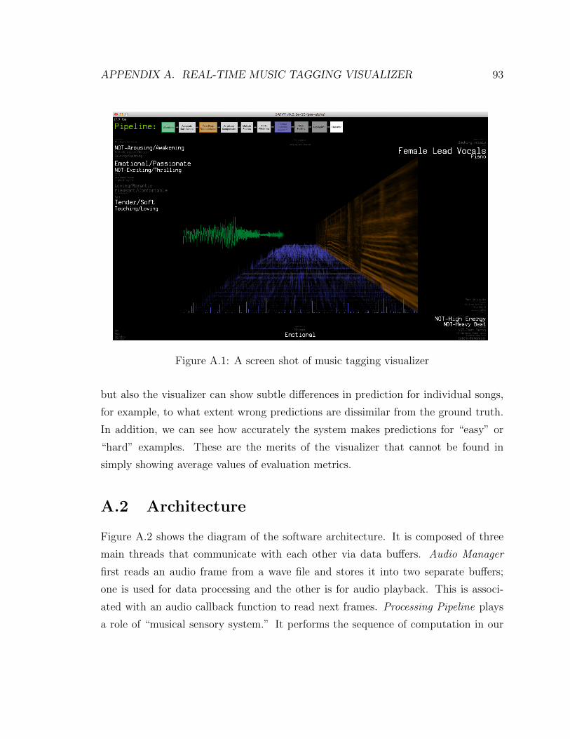
APPENDIX A. REAL-TIME MUSIC TAGGING VISUALIZER 93
Figure A.1: A screen shot of music tagging visualizer
but also the visualizer can show subtle differences in prediction for individual songs,
for example, to what extent wrong predictions are dissimilar from the ground truth.
In addition, we can see how accurately the system makes predictions for “easy” or
“hard” examples. These are the merits of the visualizer that cannot be found in
simply showing average values of evaluation metrics.
A.2 Architecture
Figure A.2 shows the diagram of the software architecture. It is composed of three
main threads that communicate with each other via data buffers. Audio Manager
first reads an audio frame from a wave file and stores it into two separate buffers;
one is used for data processing and the other is for audio playback. This is associ-
ated with an audio callback function to read next frames. Processing Pipeline plays
a role of “musical sensory system.” It performs the sequence of computation in our

APPENDIX A. REAL-TIME MUSIC TAGGING VISUALIZER 94
audio bufferAudio
ManagerProcessing
Pipeline
audio buffer�����
PlayBack
Waveform buffer
View Manager
Mel-spec buffer
Hidden-Layer buffer
Input control(e.g. select song)
key command
Tag buffer
Figure A.2: Diagram of software architecture
proposed data processing pipeline; time-frequency AGC, FFT, mel-frequency map-
ping, feature encoding and tag prediction. We used sparse RBM and linear SVM
for learning algorithms (including PCA). The feature and tags were computed using
trained parameters from the algorithms. We produced four different outputs from
the pipeline. Each of them is stored in the corresponding buffer every frame time.
Finally, View Manager fetches the buffers and visualizes them at different locations.
A.3 Implementation Details
We built the software architecture based on the following software libraries.
• SFML (Simple and Fast Multimedia Library)1 : This is a free multimedia C++
API and used for 3-D visualization (OpenGL) in View Manager.
• RtAudio2 : This is an audio library for real-time audio input/output and used
for reading wav file and playback audio frames in Audio Manager.
1SFML: http://www.sfml-dev.org2RtAudio: http://www.music.mcgill.ca/~gary/rtaudio

APPENDIX A. REAL-TIME MUSIC TAGGING VISUALIZER 95
• Eigen3: This is a C++ template library for linear algebra. We used this for ma-
trix computation, element-wise math functions and FFT in Processing Pipeline.
• libsndfile4: This is a C library for reading and writing audio files. We used this
for reading .wav files.
3Eigen: http://eigen.tuxfamily.org/4libsndfile: http://www.mega-nerd.com/libsndfile/

Appendix B
Supplementary Materials
Audio and video examples to support this thesis are maintained in this website:
https://ccrma.stanford.edu/~juhan/thesis. It contains the following content.
• Dictionary learning animation
• Music tagging visualizer demo video
• Audio examples: reconstructed outputs from the following stages in the data
processing pipeline
- Original waveform
- AGC output
- Mel-frequency spectrogram
- PCA Whitening
- Sparse RBM
96

Bibliography
[1] Samer A. Abdallah and Mark D. Plumbley. Unsupervised analysis of
polyphonic music by sparse coding. IEEE Transactions on Neural Networks,
2006.
[2] Jean-Julien Aucouturier and Franois Pachet. Representing musical genre: A
state of the art. Journal of New Music Research, 2003.
[3] Horace B. Barlow. Possible principles underlying the transformation of
sensory messages. Sensory Communication, pages 217–234, 1961.
[4] Yoshua Bengio and Hugo Larochelle Pascal Lamblin, Dan Popovici. Greedy
layer-wise training of deep networks. Advances in Neural Information
Processing Systems 19, 2007.
[5] James Bergstra, Norman Casagrande, Dumitru Erhan, Douglas Eck, and
Balazs Kegl. Aggregate features and adaboost for music classification.
Machine Learning, 2006.
[6] James Bergstra, Michael Mandel, and Douglas Eck. Scalable genre and tag
prediction using spectral covariance. In Proceedings of the 11th International
Conference on Music Information Retrieval (ISMIR), 2010.
[7] T. Bertin-Mahieux, D. Eck, F. Maillet, and P. Lamere. Autotagger: a model
for predicting social tags from acoustic features on large music databases. In
Journal of New Music Research, 2008.
97

BIBLIOGRAPHY 98
[8] Thierry Bertin-Mahieux, Dan Ellis, Brian Whitman, and Paul Lamere. The
million song dataset. In Proceedings of the 12th international society for music
information retrieval conference, 2011.
[9] Thomas Blumensath and Mike Davies. Sparse and shift-invariant
representations of music. IEEE transactions on audio, speech and language
processing, 2006.
[10] Y-Lan Boureau, Jean Ponce, and Yann LeCun. A theoretical analysis of
feature pooling in visual recognition. Proceedings of the 27th International
Conference on Machine Learning (ICML), 2010.
[11] J. S. Bridle and M. D. Brown. An experimental automatic word-recognition
system. JSRU Report No. 1003, Joint Speech Research Unit, 1974.
[12] David .J. Field Bruno. A. Olshausen. Emergence of simple-cellreceptive field
properties by learning a sparse code for natural images. Nature, pages
607–609, 1996.
[13] Michael A. Casey, Remco VeltKamp, Masataka Goto, Marc Leman,
Christophe Rhodes, and Malcolm Slaney. Content-based music information
retrieval: Current directions and future challenges. Proceedings of the IEEE,
96:668–696, 2008.
[14] Oscar Celma. Music recommendation and discovery in the long tail. PhD
thesis, Universitat Pompeu Fabra,Barcelona, Spain, 2008.
[15] Adam Coates, Blake Carpenter, Carl Case, Sanjeev Satheesh, Bipin Suresh,
Tao Wang, David J. Wu, and Andrew Y. Ng. Text detection and character
recognition in scene images with unsupervised feature learning. 2011.
[16] Adam Coates, Honglak Lee, and Andrew Ng. An analysis of single-layer
networks in unsupervised feature learning. Journal of Machine Learning
Research, 2011.

BIBLIOGRAPHY 99
[17] Adam Coates and Andrew Y. Ng. The importance of encoding versus training
with sparse coding and vector quantization. In Proceedings of the 28th
International Conference on Machine Learning (ICML), 2011.
[18] Emanuele Coviello, Antoni B. Chan, and Gert R. G. Lanckriet. Time series
models for semantic music annotation. IEEE Transactions on Audio, Speech,
and Language Processing, 2011.
[19] Emanuele Coviello, Riccardo Miotto, and Gert R. G. Lanckriet. Combining
content-based auto-taggers with decision-fusion. In Proceedings of the 12th
International Conference on Music Information Retrieval (ISMIR), 2011.
[20] Steven B. Davis and Paul Mermelstein. Comparison of parametric
representations for monosyllabic word recognition in continuously spoken
sentences. IEEE Transactions on Acoustics, Speech and Signal Processing,
1980.
[21] Sander Dieleman, Philmon Brakel, and Benjamin Schrauwen. Audio-based
music classification with a pretrained convolutional network. In Proceedings of
the 12th International Conference on Music Information Retrieval (ISMIR),
2011.
[22] Dan Ellis. A history and overview of machine listening. web resource,
available,
http://www.ee.columbia.edu/~dpwe/talks/gatsby-2010-05.pdf, 2010.
[23] Dan Ellis. Time-frequency automatic gain control. web resource, available,
http://labrosa.ee.columbia.edu/matlab/tf_agc/, 2010.
[24] Dan Ellis and Graham Poliner. Identifying cover songs with chroma features
and dynamic programming beat tracking. In Proceedings of the IEEE
International Conference on Acoustics, Speech and Signal Processing
(ICASSP), Honolulu, Hawaii, USA, 2007.
BIBLIOGRAPHY 100
[25] Daniel P. W. Ellis. PLP and RASTA (and MFCC, and inversion) in Matlab,
2005. online web resource.
[26] Katherine Ellis, Emanuele Coviello, and Gert R. G. Lanckriet. Semantic
annotation and retrieval of music using a bag of systems representation. In
Proceedings of the 12th International Conference on Music Information
Retrieval (ISMIR), 2011.
[27] Valentin Emiya, Roland Badeau, and Bertrand David. Multipitch estimation
of piano sounds using a new probabilistic spectral smoothness principle. IEEE
Transaction on Audio, Speech and Language Processing, 2010.
[28] Rong-En Fan, Kai-Wei Chang, Cho-Jui Hseigh, Xiang-Rui Wang, and
Chih-Jen Lin. LIBLINEAR: a library for large linear classification. Journal of
Machine Learning Research, 2008.
[29] Zhouyu Fu, Guojun Lu, Kai Ming Ting, and Dengsheng Zhang. On feature
combination for music classification. Proceedings of International Workshop
on Statistical Pattern Recognition, 2010.
[30] Takuya Fujishima. Realtime chord recognition of musical sound: a system
using common lisp music. In Proceedings of the International Conference on
Computer Music (ICMC), 1999.
[31] Masataka Goto. A predominant-f0 estimation method for cd recordings:map
estimation using em algorithm for adaptive tone models. In Preceedings of
IEEE International Conference on Acoustics, Speech and Signal Processing,
2001.
[32] Philippe Hamel and Douglas Eck. Learning features from music audio with
deep belief networks. In In Proceedings of the 11th International Conference
on Music Information Retrieval (ISMIR), 2010.
[33] Philippe Hamel, Simon Lemieux, Yoshua Bengio, and Douglas Eck. Temporal
pooling and multiscale learning for automatic annotation and ranking of music

BIBLIOGRAPHY 101
audio. In Proceedings of the 12th International Conference on Music
Information Retrieval (ISMIR), 2011.
[34] Philippe Hamel, Sean Wood, and Douglas Eck. Automatic identification of
instrument classes in polyphonic and poly-instrument audio. In In Proceedings
of the 10th International Conference on Music Information Retrieval
(ISMIR), 2009.
[35] Mikael Henaff, Kevin Jarrett, Koray Kavukcuoglu, and Yann LeCun.
Unsupervised learning of sparse features for scalable audio classification. In
Proceedings of the 12th International Conference on Music Information
Retrieval (ISMIR), 2011.
[36] Geoffrey E. Hinton, Simon Osindero, and Yee-Whye Teh. A fast learning
algorithm for deep belief nets. Neural computation, 18:1527–1554, 2006.
[37] Geoffrey E. Hinton and Ruslan R. Salakhutdinov. Reducing the
dimensionality of data with neural networks. Science, 2006.
[38] Matt Hoffman, David Blei, and Perry Cook. Easy as CBA: A simple
probabilistic model for tagging music. In Proceedings of the 10th International
Conference on Music Information Retrieval (ISMIR), 2009.
[39] Andr Holzapfel and Yannis Stylianou. Musical genre classication using
nonnegative matrix factorization-based features. IEEE Transactions on
Acoustics, Speech and Signal Processing, 2008.
[40] Eric J. Humphrey, Juan Pablo Bello, and Yann LeCun. Moving beyond
feature design: Deep architectures and automatic feature learning in music
informatics. In Proceedings of the 13th International Conference on Music
Information Retrieval (ISMIR), 2012.
[41] M. J. Hunt, M. Lennig, and P. Mermelstein. Experiments in syllable-based
recognition of continuous speech. In ICASSP, 1980.

BIBLIOGRAPHY 102
[42] Aapo Hyvarinen, Jarmo Hurri, and Patrik O. Hoyer. Natural Image Statistics.
Springer-Verlag, 2009.
[43] Navdeep Jaitly and Geoffrey Hinton. Learning a better representation of
speech sound waves using restricted boltzmann machines. In Proceedings of
the IEEE International Conference on Acoustics, Speech and Signal Processing
(ICASSP), 2011.
[44] Navdeep Jaitly and Geoffrey E. Hinton. A new way to learn acoustic events.
NIPS 2011 Workshop on Deep Learning and Unsupervised Feature Learning,
2011.
[45] Kaichun K. Chang Jyh-Shing Roger Jang and Costas S. Iliopoulos. Music
genre classication via compressive sampling. In Proceedings of the 11th
International Conference on Music Information Retrieval (ISMIR), 2010.
[46] D.-N. Jiang, L. Lu, H.-J. Zhang, and J.-H. Tao. Music type classification by
spectral contrast feature. In Proceedings of International Conference on
Multimedia Expo (ICME), 2002.
[47] Koray Kavukcuoglu, Marc’Aurelio Ranzato, and Yann LeCun. Fast inference
in sparse coding algorithms with applications to object recognition. Technical
Report CBLL-TR-2008-12-01, Computational and Biological Learning Lab,
Courant Institute, NYU, 2008.
[48] Anssi Klapuri. A perceptually motivated multiple-f0 estimation method. In
Proceedings of IEEE Workshop on Applications of Signal Processing to Audio
and Acoustics, 2005.
[49] Edith Law and Luis Von Ahn. Input-agreement: a new mechanism for
collecting data using human computation games. In Proc. Intl. Conf. on
Human factors in computing systems, CHI. ACM, 2009.
[50] Yann LeCun, Leon Bottou, Yoshua Bengio, and Patrick Haffner.
Gradient-based learning applied to document recognition. Proceedings of the
IEEE, 1998.

BIBLIOGRAPHY 103
[51] Chang-Hsing Lee, Jau-Ling Shih, Kun-Ming Yu, and Hwai-San Lin.
Automatic music genre classification based on modulation spectral analysis of
spectral and cepstral features. IEEE Transaction on Multimedia, 2009.
[52] Honglak Lee. Unsupervised feature learning via sparse hierarchical
representations. Ph.D thesis, Stanford University, 2010.
[53] Honglak Lee, Chaitanya Ekanadham, and Andrew Y. Ng. Sparse deep belief
net model for visual area V2. In Advances in Neural Information Processing
Systems 20, pages 873–880. 2008.
[54] Honglak Lee, Roger Grosse, Rajesh Ranganath, and Andrew Y. Ng.
Convolutional deep belief networks for scalable unsupervised learning of
hierarchical representations. In Proceedings of the 26th International
Conference on Machine Learning, pages 609–616, 2009.
[55] Honglak Lee, Yan Largman, Peter Pham, and Andrew Y. Ng. Unsupervised
feature learning for audio classification using convolutional deep belief
networks. In Advances in Neural Information Processing Systems 22, pages
1096–1104. 2009.
[56] Jong-Hwan Lee, Ho-Young Jung, Te-Won Lee, and Soo-Young Lee. Speech
feature extraction using independent component analysis. In Proceedings of
the IEEE International Conference on Acoustics, Speech and Signal Processing
(ICASSP), 2000.
[57] Michael S. Lewicki. Efficient coding of natural sounds. Nature Neuroscience,
2002.
[58] Tao Li, Mitsunori Ogihara, and Qi Li. A comparative study of content-based
music genre classification. In Proceedings of the 26th international ACM
SIGIR conference on Research and development in informaion retrieval, 2003.
[59] T. Lidy, A. Rauber, A. Pertusa, and J. Inesta. Combining audio and symbolic
descriptors for music classification from audio,. In Music Information
Retrieval Information Exchange (MIREX), 2007.

BIBLIOGRAPHY 104
[60] Dick Lyon. Machine hearing: an emerging field. IEEE Signal Processing
Magazine, 2010.
[61] Richard Lyon. Filter cascades as analogs of the cochlea. Neuromorphic
systems engineering: neural networks in silicon, 1998.
[62] Micahel Mandel and Dan Ellis. Song-level features and svms for music
classification. In Proceedings of the 6th International Conference on Music
Information Retrieval (ISMIR), 2005.
[63] Pierre-Antoine Manzagol, Thierry Bertin-Mahieux, and Douglas Eck. On the
use of sparse time-relative auditory codes for music. In Proceedings of the 9th
International Conference on Music Information Retrieval (ISMIR), 2008.
[64] Matija Marolt. A connectionist approach to automatic transcription of
polyphonic piano music. IEEE Transactions on Multimedia, 2004.
[65] Cory McKay and Ichiro Fujinaga. Musical genre classification: Is it worth
pursuing and how can it be improved? In Proceedings of the 6th International
Conference on Music Information Retrieval (ISMIR), 2006.
[66] Martin F. McKinney and Jeroen Breebaart. Features for audio and music
classification. In Proceedings of the 4th International Conference on Music
Information Retrieval (ISMIR), 2003.
[67] Brian. C. J. Moore and Brian R. Glasberg. A revision of zwicker’s loudness
model. Acta Acustica, 1996.
[68] J. Andy Moorer. On the transcription of musical sound by computer.
Computer Music Journal, 1987.
[69] Meinard Muller, Dan Ellis, Anssi Klapuri, and Gal Richard. Signal processing
for music analysis. IEEE Journal on Selected Topics in Signal Processing,
2011.

BIBLIOGRAPHY 105
[70] Meinard Muller and Sebastian Ewert. Chroma Toolbox: MATLAB
implementations for extracting variants of chroma-based audio features. In
Proceedings of the 12th International Conference on Music Information
Retrieval (ISMIR), Miami, USA, 2011.
[71] Juhan Nam, Jorge Herrera, Malcolm Slaney, and Julius O. Smith. Learning
sparse feature representations for music annotation and retrieval. In
Proceedings of the 13th International Conference on Music Information
Retrieval (ISMIR), 2012.
[72] Juhan Nam, Jiquan Ngiam, Honglak Lee, and Malcolm Slaney. A
classification-based polyphonic piano transcription approach using learned
feature representation. In Proceedings of the 12th International Conference on
Music Information Retrieval (ISMIR), 2011.
[73] Andrew Ng. Unsupervised feature learning and deep learning. web resource,
available, http://icml2011speechvision.files.wordpress.com/2011/06/
visionaudio.pdf, 2011.
[74] Andrew Y. Ng. CS294A lecture note: Sparse autoencoder.
[75] Andrew Y. Ng and Michael I. Jordan. On discriminative vs. generative
classifiers: A comparison of logistic regression and naive bayes. Advances in
Neural Information Processing Systems 14, 2001.
[76] J. Ngiam, P. Koh, Z. Chen, S. Bhaskar, and A.Y. Ng. Sparse filtering.
Proceedings of the 25th Conference on Neural Information Processing Systems
(NIPS), 2011.
[77] Jiquan Ngiam, Aditya Khosla, Mingyu Kim, Juhan Nam, Honglak Lee, and
Andrew Y. Ng. Multimodal deep learning. In Proceedings of the 28th
International Conference on Machine Learning (ICML), June 2011.
[78] Bruno A. Olshausen and David J. Field. Sparse coding with an overcomplete
basis set: a strategy employed by v1. Vision Research, 37:3311–3325, 1997.

BIBLIOGRAPHY 106
[79] Elias Pampalk, Arthur Flexer, and Gerhard Widmer. Improvements of
audio-based music similarity and genre classification. In Proceedings of the 6th
International Conference on Music Information Retrieval (ISMIR), 2005.
[80] Elias Pampalk, Andreas Rauber, and Dieter Merkl. Content-based
organization and visualization of music archives. In Proceedings of ACM
Multimedia, 2002.
[81] Yannis Panagakis, Constantine Kotropoulos, and Gonzalo R. Arce. Music
genre classification using locality preserving nonnegative tensor factorization
and sparse representations. In Proceedings of the 10th International
Conference on Music Information Retrieval (ISMIR), 2009.
[82] Yannis Panagakis, Constantine Kotropoulos, and Gonzalo R. Arce. Music
genre classification via sparse representation of auditory temporal
modulations. In Proceedings of the 17th European Signal Processing
Conference (EUSIPCO), 2009.
[83] Yannis Panagakis, Constantine Kotropoulos, and Gonzalo R. Arce.
Non-negative multilinear principal component analysis of auditory temporal
modulations for music genre classification. IEEE Transaction on Audio,
Speech and Language Processing, 2010.
[84] Roy D. Patterson, Mike H. Allerhand, and Christian Giguere. Time-domain
modelling of peripheral auditory processing: A modular architecture and
software platform. Journal of the Acoustical Society of America, 1995.
[85] Graham E. Poliner and D. Ellis. A discriminative model for polyphonic piano
transcription. EURASIP Journal on Advances in Signal Processing, 2007.
[86] Graham E. Poliner and D. Ellis. Improving generalization for
classification-based polyphonic piano transcription. In Proceedings of IEEE
Workshop on Applications of Signal Processing to Audio and Acoustics, 2007.

BIBLIOGRAPHY 107
[87] Matti Ryynnen and Anssi Klapuri. Polyphonic music transcription using note
event modeling. In Proceedings of IEEE Workshop on Applications of Signal
Processing to Audio and Acoustics, 2005.
[88] Ruslan Salakhutdinov and Geoffrey Hinton. Semantic hashing. International
Journal of Approximate Reasoning, 2009.
[89] Andrew I. Schein, Alexandrin Popescul, Lyle H. Ungar, and David M.
Pennock. Methods and metrics for cold-start recommendations. In
Proceedings of the 25th annual international ACM SIGIR conference on
Research and development in information retrieval, SIGIR ’02, pages 253–260,
New York, NY, USA, 2002. ACM.
[90] Jan Schluter and Christian Osendorfer. Music Similarity Estimation with the
Mean-Covariance Restricted Boltzmann Machine. In Proceedings of the 10th
International Conference on Machine Learning and Applications, 2011.
[91] Erik M. Schmidt and Youngmoo E. Kim. Learning emotion-based acoustic
features with deep belief networks. In Proceedings of the 2011 IEEE Workshop
on Applications of Signal Processing to Audio and Acoustics (WASPAA),
2011.
[92] Erik M. Schmidt, Jeffrey Scott, and Youngmoo E. Kim. Feature learning in
dynamic environments:modeling the acoustic structure of musical emotion. In
Proceedings of the 13th International Conference on Music Information
Retrieval (ISMIR), 2012.
[93] Malcolm Slaney. Auditory toolbox-version 2, 1998. online web resource.
[94] Malcolm Slaney. Web-scale multimedia analysis: Does content matter? IEEE
Multimedia, 18, 2011.
[95] Paris Smaragdis and Judy C. Brown. Non-negative matrix factorization for
polyphonic music transcription. In Proceedings of IEEE Workshop on
Applications of Signal Processing to Audio and Acoustics, 2003.

BIBLIOGRAPHY 108
[96] Evan Smith and Michael S. Lewicki. Efficient auditory coding. Nature, 2006.
[97] Julius Smith. Spectral Audio Signal Processing. W3K Publishing, 2011.
[98] Paul Smolensky. Information processing in dynamical systems:foundation of
harmony theory. In Parallel Distributed Processing: explorations in the
microstructure of cognition, vol. 1, pages 194–281. MIT Press, Cambridge,
1986.
[99] Stanley Smith Stevens, John Volkman, and Edwin Newman. A scale for the
measurement of the psychological magnitude pitch. Journal of the Acoustical
Society of America, 1937.
[100] K. Trohidis, G. Tsoumakas, G. Kalliris, and I. Vlahavas. Multilabel
classification of music into emotions. In Proceedings of the 9th International
Conference on Music Information Retrieval (ISMIR), 2008.
[101] Douglas Turnbull, Luke Barrington, and Gert Lanckriet. Modeling music and
words using a multi-class naive bayes approach. In Proceedings of the 7th
International Conference on Music Information Retrieval (ISMIR), 2006.
[102] Douglas Turnbull, Luke Barrington, David Torres, and Gert Lanckriet.
Towards musical query-by-semantic description using the CAL500 data set. In
ACM Special Interest Group on Information Retrieval Conference, 2007.
[103] Douglas Turnbull, Luke Barrington, David Torres, and Gert R. G. Lanckriet.
Semantic annotation and retrieval of music and sound effects. IEEE
Transactions on Audio, Speech, and Language Processing, 2008.
[104] George Tzanetakis and Perry Cook. Musical genre classification of audio
signals. IEEE Transaction on Speech and Audio Processing, 2002.
[105] George Tzanetakis, Randy Jones, and Kirk McNally. Stereo panning features
for classifying recording production style. In Proceedings of the 8th
International Conference on Music Information Retrieval (ISMIR), 2007.

BIBLIOGRAPHY 109
[106] C. G. v. d. Boogaart and R. Lienhart. Note onset detection for the
transcription of polyphonic piano music. In Preceedings of IEEE International
Conference on Multimedia and Expo, 2009.
[107] Emmanuel Vincent, Nancy Bertin, and Roland Badeau. Adaptive harmonic
spectral decomposition for multiple pitch estimation. IEEE Transaction on
Audio, Speech and Language Processing, 2010.
[108] Gregory H. Wakefield. Mathematical representation of joint time-chroma
distributions. In SPIE, Denver, Colorado, 1999.
[109] Erling Wold, Thom Blum, Douglas Keislar, and James Wheaton.
Content-based classification, search, and retrieval of audio. IEEE MultiMedia,
3(3):27–36, 1996.
[110] Tong Tong Wu and Kenneth Lange. Coordinate descent algorithms for lasso
penalized regression. Annals of Applied Statistics, 2008.
[111] Jan Wulng and Martin Riedmiller. Unsupervised learning of local features for
music classification. In Proceedings of the 13th International Conference on
Music Information Retrieval (ISMIR), 2012.
[112] Bo Xie, Wei Bian, Dacheng Tao, and Parag Chordia. Music tagging with
regularized logistic regression. In Proceedings of the 12th International
Conference on Music Information Retrieval (ISMIR), 2011.
[113] Eberhard Zwicker. A scale for the measurement of the psychological
magnitude pitch. Journal of the Acoustical Society of America, 1961.