learning from data

Learning from Data

Russell and Norvig Chapter 18

Learning

n  Essential for agents working in unknown environments

n  Learning is useful as a system construction method q  Expose the agent to reality rather than trying to

write it down

n  Learning modifies the agent's decision mechanisms to improve performance

Learning from examples

n  Supervised learning: Given labeled examples of each digit, learn a classification rule

Machine learning is ubiquitous

n  Examples of systems that employ ML?

Examples of learning tasks

n  OCR (Optical Character Recognition) n  Loan risk diagnosis n  Medical diagnosis n  Credit card fraud detection n  Speech recognition (e.g., in automatic call handling systems) n  Spam filtering n  Collaborative filtering (recommender systems) n  Biometric identification (fingerprints, iris scan, face) n  Information retrieval (incl. web searching) n  Data mining, e.g. customer purchase behavior n  Customer retention n  Bioinformatics: prediction of properties of genes and proteins.

Learning

n  The agent tries to learn from the data (examples) provided to it.

n  The agent receives feedback that tells it how well it is doing. n  There are several learning scenarios according to the type of

feedback: q  Supervised learning: correct answers for each example q  Unsupervised learning: correct answers not given q  Reinforcement learning: occasional rewards (e.g. learning to play

a game). n  Each scenario has appropriate learning algorithms

ML tasks

Classification: discrete/categorical labels Regression: continuous labels Clustering: no labels

7 0 2 4 6 8 10 12 142

4

6

8

10

12

14

16

Inductive learning

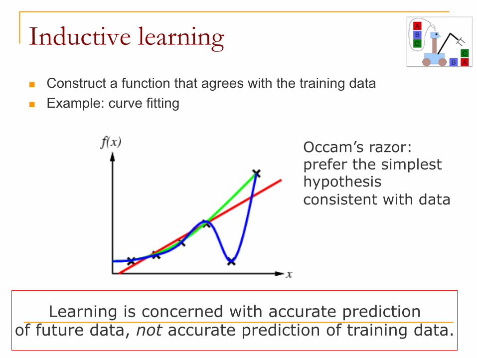
n  Construct a function that agrees with the training data n  Example: curve fitting

Inductive learning

n  Construct a function that agrees with the training data n  Example: curve fitting

Which of these models do you think is better?

Inductive learning

n  Construct a function that agrees with the training data n  Example: curve fitting Occam’s razor:

prefer the simplest hypothesis consistent with data

Learning is concerned with accurate prediction of future data, not accurate prediction of training data.

Occam’s Razor

http://old.aitopics.org/AIToons

Overfitting in classification

Supervised Learning

Example: want to classify versus

Data: Labeled images

xi is a vector of features that represents the the image

Task: Here is a new image: What species is it?

D = {(xi, yi)}ni=1

The Nearest Neighbor Method (your first classification algorithm!)

NN(image): 1.  Find the image in the training data which is closest to

the query image. 2.  Return its label.

query closest image

Distance measures

n  How to measure closeness?

Distance measures

n  How to measure closeness?

n  Discrete data: Hamming distance n  Continuous data: Euclidean distance n  Sequence data: edit distance

n  Alternative: use a similarity measure (or dot product) rather than a distance

k-NN

n  Use the closest k neighbors to make a decision instead of a single nearest neighbor

n  Why do you expect this to work better?

Remarks on Nearest Neighbor n  Very easy to implement n  No training required. All the computation performed in

classifying an example (complexity: O(n) ) n  Need to store the whole training set (memory inefficient). n  Flexible, no prior assumptions (a type of non parametric

classifier: does not assume anything about the data). n  Curse of dimensionality: if data has many features that

are irrelevant/noisy distances are always large.

Take home question

n  How would you convert the k-nearest-neighbor classification method to a regression method?

Measuring classifier performance

n  Or how accurate is my classifier.


n  The error-rate on a set of examples :

n  What is the error rate of a nearest neighbor classifier applied to its training set?

n  Accuracy is 1-(error-rate)

I is the indicator function that returns 1 if its argument is True and zero otherwise

D = {(xi, yi)}ni=1



n  Report error rates computed on an independent test set (classifier was trained using training set): classifier performance on the training set is not indicative of performance on unseen data.


D = {(xi, yi)}ni=1



n  Issue when classes are imbalanced. n  There are other measures of performance that

address this.


D = {(xi, yi)}ni=1


n  Split data into training set and test set (say 70%, 30%).

n  Compare several classifiers trained on this split. n  Train final best classifier on the full dataset.

n  A better method: cross-validation

Cross-validation

n  Split data into k parts (E1,…,Ek) for i = 1,…,k : training set = D\Ei

test set = Ei classifier.train(training set) accumulate results of classifier.test(test set)

n  This is called k-fold cross-validation n  Extreme version: Leave-One-Out n  Assumptions?

Uses of CV

Cross Validation is used to choose: n  Classifier parameters

q  k for k-NN n  Normalization method n  Which classifier n  Feature selection (which features provide

best performance). n  This is called model selection

CV-based model selection

n  We’re trying to determine which classifier to use

Classifier Training error

CV-error choice

f1 f2

f3 ✔

f4

f5

f6

CV-based model selection

n  Example: choosing k for the k-NN algorithm:

Classifier Training error

CV-error choice

K = 1 K = 2

K = 3 ✔

K = 4

K = 5

K = 6

The general workflow

n  Formulate problem n  Get data n  Decide on a representation (what features to

use) n  Visualize the data n  Choose a classifier n  Assess the performance of the classifier n  Depending on the results: modify the

representation, classifier, or look for more data

Decision Tree Learning

Russell and Norvig Chapter 18.3

Learning decision trees

Problem: decide whether to wait for a table at a restaurant, based on the following attributes: 1.  Alternate: is there an alternative restaurant nearby? 2.  Bar: is there a comfortable bar area to wait in? 3.  Fri/Sat: is today Friday or Saturday? 4.  Hungry: are we hungry? 5.  Patrons: number of people in the restaurant (None, Some, Full) 6.  Price: price range ($, $$, $$$) 7.  Raining: is it raining outside? 8.  Reservation: have we made a reservation? 9.  Type: kind of restaurant (French, Italian, Thai, Burger) 10.  WaitEstimate: estimated waiting time (0-10, 10-30, 30-60, >60)

Attribute-based representations n  Examples described by attribute values (Boolean, discrete, continuous) n  Example: situations where I will/won't wait for a table:

n  Examples are labeled as positive (T) or negative (F)

Decision trees

n  Decision trees: a form of representation for hypotheses (classification rules)

n  Example: the “true” tree for deciding whether to wait:

Expressiveness

n  Decision trees can express any function of the input attributes. n  E.g., for Boolean functions, truth table row → path to leaf:

n  Trivially, there is a consistent decision tree for any training set with one path to leaf for each example but it probably won't generalize to new examples

n  Prefer to find compact decision trees

Decision tree learning

n  Aim: find a small tree consistent with the training examples n  Idea: (recursively) choose "most significant" attribute as root of (sub)tree

Choosing an attribute

n  Idea: a good attribute splits the examples into subsets that are (ideally) "all positive" or "all negative"

n  Patrons? is a better choice n  Need a measure of quality for an attribute

Digression: information theory

n  I am thinking of an integer between 0 and 1,023. You want to guess it using the fewest number of questions.

n  Most of us would ask “is it between 0 and 512?” n  This is a good strategy because it provides the most

information about the unknown number. n  It provides the first binary digit of the number. n  Initially you need to obtain log2(1024) = 10 bits of

information. After the first question you only need log2(512) = 9 bits.

Information theory (cont).

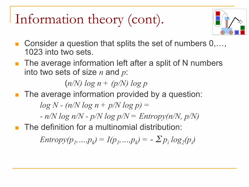
n  Consider a question that splits the set of numbers 0,…,1023 into two sets.

n  The average information left after a split of N numbers into two sets of size n and p: (n/N) log n + (p/N) log p

n  The average information provided by a question: log N - (n/N log n + p/N log p) = - n/N log n/N - p/N log p/N = Entropy(n/N, p/N)

n  The definition for a multinomial distribution: Entropy(p1,…,pk) = I(p1,…,pk) = - Σ pi log2(pi)

Entropy

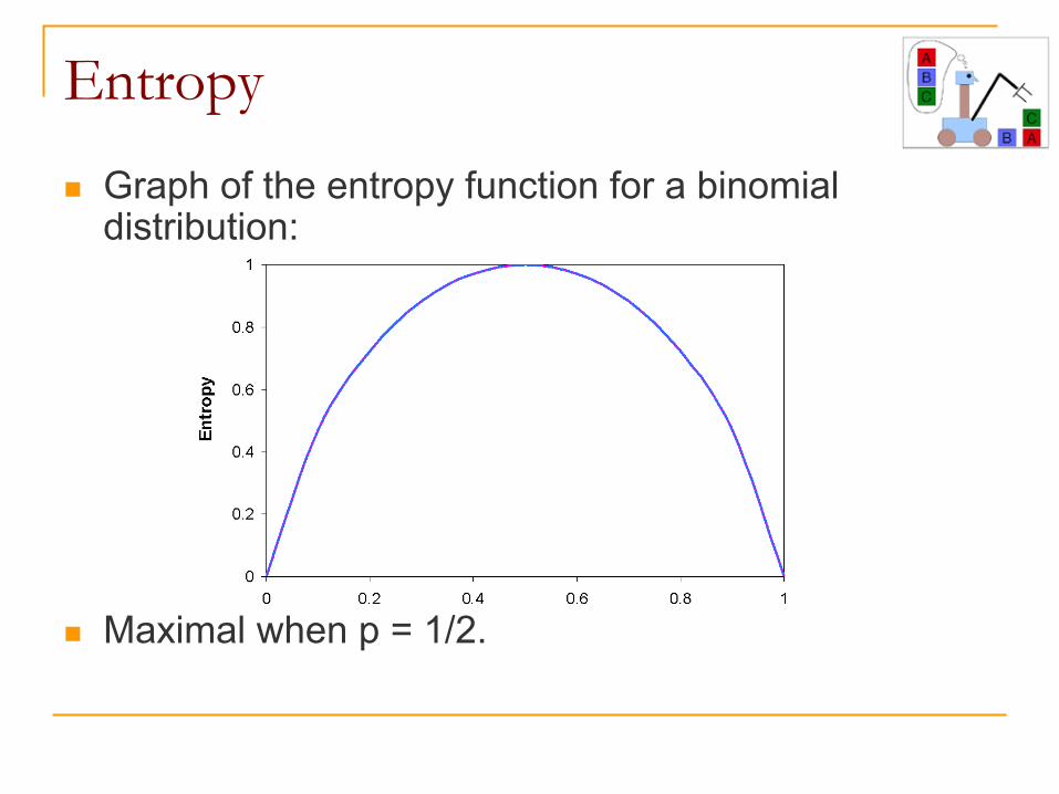
n  Graph of the entropy function for a binomial distribution:

n  Maximal when p = 1/2.

Example: triangles and squares

. .

. .

.

.

# ShapeColor Outline Dot

1 green dashed no triange2 green dashed yes triange3 yellow dashed no square4 red dashed no square5 red solid no square6 red solid yes triange7 green solid no square8 green dashed no triange9 yellow solid yes square10 red solid no square11 green solid yes square12 yellow dashed yes square13 yellow solid no square14 red dashed yes triange

Attribute

Data Set: A set of classified objects

Entropy

•  5 triangles •  9 squares •  class probabilities

•  entropy

. .

. .

.

.

. .

. .

.

.

. .

. .

.

.

red

yellow

green

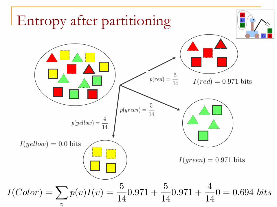
Entropy after partitioning

Reduction in entropy by partitioning

. .

. .

.

.

. .

. .

.

.

red

yellow

green

Entropy after partitioning

. .

. .

.

.

. .

. .

.

.

red

yellow

green

Information Gain

Information Gain

n  Attributes q  IG(Color) = 0.246 q  IG(Outline) = 0.151 q  IG(Dot) = 0.048

n  Heuristic: attribute with the highest gain is chosen for making a split

. .

. .

.

. . .

. .

.

.

Color?

red

yellow green

dashed

solid

Dot? no

yes

Outline? Gain(Outline) = 0.971 – 0 = 0.971 bits Gain(Dot) = 0.971 – 0.951 = 0.020 bits

Example

. .

. .

.

. . .

. .

.

.

Color?

red

yellow green

.

. dashed

solid

Dot? no

yes

Outline?

Gain(Outline) = 0.971 – 0.951 = 0.020 bits Gain(Dot) = 0.971 – 0 = 0.971 bits

Example (cont.)

. .

. .

.

. . .

. .

.

.

Color?

red

yellow green

.

. dashed

solid

Dot? no

yes

. .

Outline?

Example (cont.)

Decision Tree

Color

Dot Outline square

red yellow

green

square triangle

yes no

square triangle

dashed solid

. .

. .

.

.

Issue with IG

n  IG favors attributes with many values n  Such attribute splits S to many subsets, and if these are small,

they will tend to be pure anyway n  One way to rectify this is through a corrected measure of

information gain ratio: GainRatio(A) = IG(A) / IntrinsicInfo(A)

IntrinsicInfo(A) Is the entropy associated with the distribution of the attribute: I(p1,…,pk) where pi is the probability of observing the ith value of A.

A |v(A)| Gain(A) GainRatio(A)

Color 3 0.247 0.156

Outline 2 0.152 0.152

Dot 2 0.048 0.049

Information Gain and Information Gain Ratio

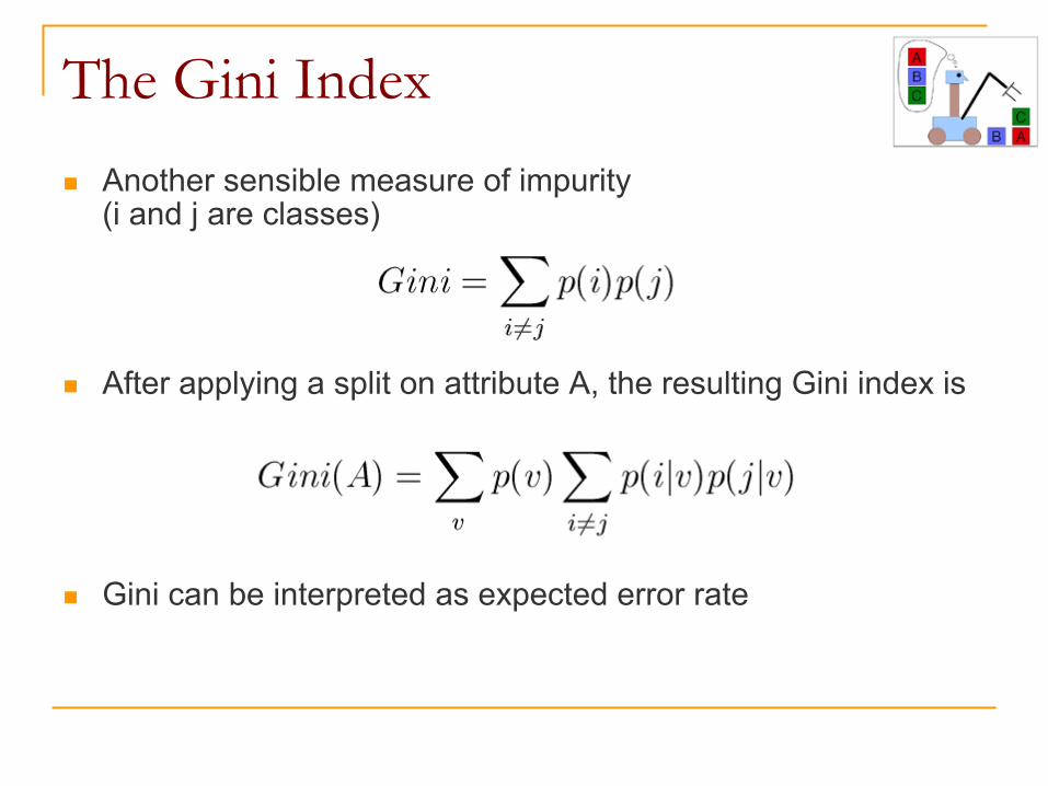
The Gini Index

n  Another sensible measure of impurity (i and j are classes)

n  After applying a split on attribute A, the resulting Gini index is

n  Gini can be interpreted as expected error rate

The Gini Index: example

. .

. .

.

.

. .

. .

.

.

. .

. .

.

.

Color?

red

yellow

green

The Gini Index: example (cont.)

The Gini Gain Index

Three Impurity Measures

A Gain(A) GainRatio(A) GiniGain(A)

Color 0.247 0.156 0.058

Outline 0.152 0.152 0.046

Dot 0.048 0.049 0.015

•  These impurity measures assess the effect of a single attribute

•  Criterion “most informative” that they define is local (and “myopic”)

•  It does not reliably predict the effect of several attributes applied jointly

Back to the restaurant example

n  Decision tree learned from the 12 examples:

n  Substantially simpler than “true” tree - a more complex hypothesis isn’t justified by small amount of data

Continuous variables

n  If variables are continuous we can bin them. n  Alternative: learn a simple classifier on a single

dimension, e.g. find decision point, classifying all data to the left in one class and all data to the right in the other

attribute i

threshold -1

+1

So, we choose an attribute, a sign “+/-” and and a threshold. This determines a half space to be +1 and the other half -1.

θ -1 +1 -1

θ

When to Stop?

n  If we keep splitting until perfect classification we might over-fit.

n  Heuristics: q  Stop when splitting criterion is below some threshold q  Stop when number of examples in each leaf node is below

some threshold

n  Alternative: prune the tree; potentially better than stopped splitting, since split may be useful at a later point.

Comments on decision trees

n  Fast training (complexity?) n  Established commercial software (e.g. CART,

C4.5, C5.0) n  Users like them because they produce rules

which can supposedly be interpreted (but decision trees are very sensitive with respect to training data)

n  Able to handle missing data (how?)

When are decision trees useful?

n  Limited accuracy for problems with many variables. Why?

Classification by committee

n  An example of a committee classifier: a classifier that bases its prediction on a set of classifiers.

n  Output: a majority vote n  If the errors made by the individual classifiers

are independent the committee will perform well.

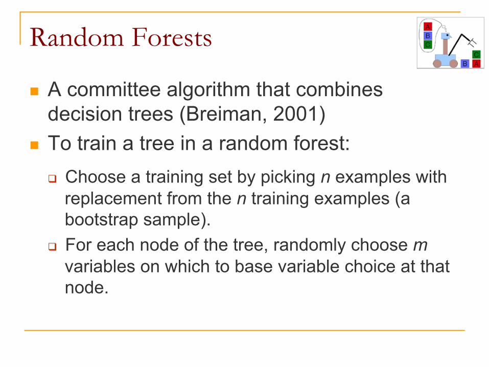
Random Forests

n  A committee algorithm that combines decision trees (Breiman, 2001)

n  To train a tree in a random forest: q  Choose a training set by picking n examples with

replacement from the n training examples (a bootstrap sample).

q  For each node of the tree, randomly choose m variables on which to base variable choice at that node.

Advantages of random forests

n  State of the art performance n  Works well for high dimensional data. n  Estimates the importance of variables in

determining classification. n  It generates an estimate of the generalization

error as the forest building progresses. n  Handles missing data well. n  Scalable to large datasets.

Bagging

n  The idea behind random forests can be applied to any classifier and is called bagging: q  Choose M bootstrap samples. q  Train M different classifiers on these bootstrap samples. q  For a new query, average or take a majority vote.

n  Other committee methods: Boosting (Freund & Schapire, 1995)

Classification: summary

n  Classifiers we learned: q  Nearest neighbors q  Decision trees q  Random forests

Next

More classifiers: n  Naïve Bayes

learning from data

Documents