learning hidden variables in probabilistic graphical...
TRANSCRIPT

LEARNING HIDDEN VARIABLES INPROBABILISTIC GRAPHICAL MODELS
THESIS SUBMITTED FOR THE DEGREE OF “DOCTOR OF PHILOSOPHY”
BY
Gal Elidan
SUBMITTED TO THE SENATE OF THE HEBREW UNIVERSITY
DECEMBER 2004

This work was carried out under the supervision of
Prof. Nir Friedman
ii

Abstract
In the past decades, a great deal of research has focused on learning probabilistic graphical
models from data. A serious problem in learning such models is the presence of hidden, or latent,
variables. These variables are not observed, yet their interaction with the observed variables has im-
portant consequences in terms of representation, inference and prediction. Consequently, numerous
works have been directed towards learning probabilistic graphical models with hidden variables. A
significantly harder challenge is that of detecting new hidden variables and incorporating them into
the network structure. Surprisingly, and despite the recognized importance of hidden variables both
in social sciences and the learning community, this problem has received little attention.
In this dissertation we explore the problem of learning new hidden variable in real-life domains.
We present methods for coping with the different elements that this task encompasses: the detection
of new hidden variables; determining the cardinality of new hidden variables; incorporating new
hidden variables into learning model. In addition we also address the problem of local maxima that
is common in many learning scenarios, and is particularly acute in the presence of hidden variables.
We present simple and easy to implement methods that work when training data is relatively
plentiful as well as a more elaborate framework that is suitable when the model is particularly
complex and the data is sparse. We also consider methods specifically tailored at networks with
continuous variables and the added challenges in this scenario.
We evaluate all of our methods on both synthetic and real-life data. For the more elaborate
methods, we put a particular emphasis on learning complex models with many hidden variables.
We demonstrate significant improvement in quantitative prediction on unseen test samples when
learning with hidden variables, reaffirming their importance in practice. We also demonstrate that
models learned with our methods have hidden variables that are qualitatively appealing and shed
light on the learned domain.

Acknowledgments
I am indebted to my adviser Nir Friedman who had a profound influence on my research. Nir
exposed me to the world of graphical models and flamed my ambition to discover hidden variables. I
have learned from Nir, a brilliant scientist, an endless collection of scientific skills: how to approach
a complex problem; how to take an idea and make it concrete; how to crisply analyze and understand
results; how to go back to data where answers (or more questions) are to be found; how to be critical
of myself but always in a constructive way; and the list goes on and on. I truly feel that I have learned
from a master and I am sure the principles Nir ingrained in me will help me throughout my career.
I was always impressed, and through the years came to appreciate even more, how hands-on Nir’s
mentoring is and how involved he is in every detail of the research from the fundamental ideas to
the axis on a figure of a presentation. Finally, while Nir was being my intellectual mentor he was
also, often on the same day, a friend. I have gossiped, dined, hiked, biked and dived with Nir. I
cannot but feel extremely lucky that I have had such an inspiring adviser.
I would like to thank, from the bottom of my heart, Eli Shamir, my first adviser. An intellectual
role-model and a person who constantly thinks of others, Eli had the insight and confidence to
direct me to a then new faculty member whose research interest better matched mine. Throughout
my studies, he continued to support and advise. I will always remember the kindness Eli showed in
taking the time to think of what is best for me, and his wisdom to push me in the right direction.
I want to thank the other members of my research committee. Yehoshua Sagiv was continuously
supportive. Dan Geiger, unknowingly, influenced my career when he gave a superb AI course.
Special thanks to the people of the Horowitz foundation for the generous support that allowed me
to invest myself in research, and to Intel corporation who provided additional support. I would also
like to thank Zvi Gilula for giving me insight to real science, for his unfaltering moral support, and
for believing in me. He was always there to help, professionally and as a friend.
I had the pleasure of fruitful collaborations with wonderful people. Noam Lotner helped make
my first paper happen, and made working together so easy. Daphne Koller, from the start, inspired
me by her intellect and impressed me with her genuine desire to listen to the ideas of a young
student. Daphne continued to collaborate, influence and support me throughout my studies and gra-
ciously took me under her wing as a postdoc. Dana Pe’er and Aviv Regev showed me how exciting
ii

computational biology can be and how far you can get when people work together. Matan Ninio
knew how to ask dumbfounding questions that constantly improved our work. Dale Schuurmans
made us feel like great scientists and helped us do great work. Yoseph Barash and Tommy Kaplan
redefined cooperation and, I hope, paved the way for many works still to come. Iftach Nachman
was always laid back yet sharp so that writing a serious paper was carefree. Ariel Jaimovich and
Hana Margalit made the last paper in my Ph.D. studies such a friendliness based success.
I spent six wonderful years at the computer science department at the Hebrew university and
worked with wonderful people. Thank you Yael, Ziva, Silvi, Regina, Rina, Lital, Ayelet, Relly,
Hagit, Koby and Eli for your friendliness and for going out of your way to help me, so that I never
felt the weight of bureaucracy. I want to thank Eli Shamir, Tali Tishby, Yoram Singer, Nir Friedman
and Yair Weiss for creating a world class learning lab that strives for excellence and at the same
time maintains a friendly atmosphere, where students are listened to, and faculty doors are always
open. I want to thank Yair for giving me an eye-opening experience as his teaching assistant. I
was fortunate to be a member of a special lab where friendship invigorates research. All current
and former lab members, including Noam S., Ran, Gill, Gal, Amir G., Lavi, Amir N., Yevgeni and
Yossi, were there to drink coffee and so much more. Koby “learned learning” with me and were
there for endless thought provoking discussions. Shai was willing to advise about linear algebra,
Hazzanic music and the nature of god. Ofer was always ready to be passionate about anything and
everything. Elon gave me a “glimpse” to political conscience.
I was also lucky to be a part of Nir’s group, a small family. Tal and Noam were with me from
the beginning and I will always consider them my friends. Ori, Hillel, Omri, Tomer, Yuval and Ilan
made every day so enjoyable. Dana was there to talk, support and care. Noa and Ariel, so quickly,
naturally and deservedly became a part of us all and made us smile. Matan made everything exciting
and was always ready to be a friend. Iftach gave me a fresh perspective on life and inspired me with
his big heart. Finally, my roommates, collaborators and friends, Tommy and Yoseph. We talked
about everything. Just by being there you made this era of my life so memorable.
I want to thank my wonderful family. My younger sister Orly who gave me constant support
by her appreciation of who I am. My big brother Sharon who from an early age encouraged my
curiosity and tirelessly challenged me to think. My parents Sara and Yossi who fed the flame within
me and somehow found the time to answer my endless questions. It is because of all of you that I
have come this far. I will forever be grateful.
Last, I am at a loss for words on how to thank my eternal love Tali. George Eliot once wrote:
“What greater thing is there for two human souls than to feel that they are joined... to strengthen
each other... to be at one with each other in silent unspeakable memories”. How right he was! Tali,
I have met you when I started my graduate studies and you have given me all that and more. You
have strengthened me and were with me in all moments and memories, silent or not. For everything
that was and will be, thank you.
iii

To my parents who supported and loved me unconditionally
and to Itai, my son, who I hope will one day feel as I do.
iv

Contents
Acknowledgments ii
1 Introduction 1
1.1 Probabilistic Graphical Models . . . . . . . . . . . . . . . . . . . . . . . . . . . . 1
1.2 Hidden Variables . . . . . . . . . . . . . . . . . . . . . . . . . . . . . . . . . . . 4
1.3 Road Map of Our Methods . . . . . . . . . . . . . . . . . . . . . . . . . . . . . . 6
2 Probabilistic Graphical Models 9
2.1 The Bayesian Network Model . . . . . . . . . . . . . . . . . . . . . . . . . . . . 10
2.1.1 Encoding Independencies . . . . . . . . . . . . . . . . . . . . . . . . . . 10
2.1.2 Independence Map (I-map) . . . . . . . . . . . . . . . . . . . . . . . . . . 13
2.1.3 Model Definition . . . . . . . . . . . . . . . . . . . . . . . . . . . . . . . 14
2.1.4 Inference . . . . . . . . . . . . . . . . . . . . . . . . . . . . . . . . . . . 16
2.2 Learning Parameters with Complete Data . . . . . . . . . . . . . . . . . . . . . . 17
2.2.1 Maximum Likelihood Estimation . . . . . . . . . . . . . . . . . . . . . . 17
2.2.2 Bayesian Estimation . . . . . . . . . . . . . . . . . . . . . . . . . . . . . 19
2.3 Structure Learning . . . . . . . . . . . . . . . . . . . . . . . . . . . . . . . . . . 21
2.3.1 The Bayesian Dirichlet Equivalent Sample Size Score . . . . . . . . . . . 22
2.3.2 Scores For Continuous CPDs . . . . . . . . . . . . . . . . . . . . . . . . . 25
2.3.3 Search Algorithm . . . . . . . . . . . . . . . . . . . . . . . . . . . . . . . 25
2.4 Learning with Missing Values and Hidden Variables . . . . . . . . . . . . . . . . . 27
2.4.1 Parameter Estimation . . . . . . . . . . . . . . . . . . . . . . . . . . . . . 28
2.4.2 Structure Learning . . . . . . . . . . . . . . . . . . . . . . . . . . . . . . 29
3 Weight Annealing 32
3.1 Annealing Algorithms . . . . . . . . . . . . . . . . . . . . . . . . . . . . . . . . 33
3.2 Weight Annealing . . . . . . . . . . . . . . . . . . . . . . . . . . . . . . . . . . . 34
3.3 Reweighting Strategies . . . . . . . . . . . . . . . . . . . . . . . . . . . . . . . . 36
3.3.1 Random Reweighting . . . . . . . . . . . . . . . . . . . . . . . . . . . . . 36
v

3.3.2 Adversarial Reweighting . . . . . . . . . . . . . . . . . . . . . . . . . . . 37
3.4 Analysis of a Toy problem . . . . . . . . . . . . . . . . . . . . . . . . . . . . . . 39
3.5 Learning Bayesian Networks . . . . . . . . . . . . . . . . . . . . . . . . . . . . . 44
3.5.1 Perturbing Structure Search . . . . . . . . . . . . . . . . . . . . . . . . . 44
3.5.2 Perturbing Parametric EM . . . . . . . . . . . . . . . . . . . . . . . . . . 46
3.5.3 Perturbing Structural EM . . . . . . . . . . . . . . . . . . . . . . . . . . . 48
3.5.4 Evaluation of real-life domains . . . . . . . . . . . . . . . . . . . . . . . . 49
3.6 Learning Sequence Motifs . . . . . . . . . . . . . . . . . . . . . . . . . . . . . . 50
3.7 Relation to Other Methods . . . . . . . . . . . . . . . . . . . . . . . . . . . . . . 52
3.8 Discussion . . . . . . . . . . . . . . . . . . . . . . . . . . . . . . . . . . . . . . . 53
4 Discovering Hidden Variables: A Structure-Based Approach 55
4.1 Detecting Hidden Variables . . . . . . . . . . . . . . . . . . . . . . . . . . . . . . 57
4.2 Experimental Results . . . . . . . . . . . . . . . . . . . . . . . . . . . . . . . . . 62
4.3 Discussion . . . . . . . . . . . . . . . . . . . . . . . . . . . . . . . . . . . . . . . 68
5 Adapting the cardinality of hidden variables 70
5.1 Learning the Cardinality of a Hidden Variable . . . . . . . . . . . . . . . . . . . . 71
5.1.1 The Agglomeration Procedure . . . . . . . . . . . . . . . . . . . . . . . . 72
5.1.2 Scoring of a Merge . . . . . . . . . . . . . . . . . . . . . . . . . . . . . . 75
5.1.3 Initialization . . . . . . . . . . . . . . . . . . . . . . . . . . . . . . . . . 76
5.2 Properties of the Score . . . . . . . . . . . . . . . . . . . . . . . . . . . . . . . . 79
5.3 Learning the Cardinality of Several Hidden Variables . . . . . . . . . . . . . . . . 80
5.4 Experimental Results and Evaluation . . . . . . . . . . . . . . . . . . . . . . . . . 81
5.5 Discussion and Previous Work . . . . . . . . . . . . . . . . . . . . . . . . . . . . 86
6 Information BottleNeck EM 89
6.1 Multivariate Information Bottleneck . . . . . . . . . . . . . . . . . . . . . . . . . 91
6.2 Information Bottleneck Expectation Maximization . . . . . . . . . . . . . . . . . 94
6.2.1 The Information Bottleneck EM Lagrangian . . . . . . . . . . . . . . . . . 94
6.2.2 The Information Bottleneck EM Algorithm . . . . . . . . . . . . . . . . . 97
6.3 Bypassing Local Maxima using Continuation . . . . . . . . . . . . . . . . . . . . 98
6.4 Multiple Hidden Variables . . . . . . . . . . . . . . . . . . . . . . . . . . . . . . 102
6.5 Proofs and Technical Computations . . . . . . . . . . . . . . . . . . . . . . . . . 105
6.5.1 Fixed point equations:Single Hidden Variable . . . . . . . . . . . . . . . . 105
6.5.2 Fixed point equations:Multiple Hidden Variable . . . . . . . . . . . . . . . 107
6.5.3 Computing the Continuation Direction . . . . . . . . . . . . . . . . . . . . 108
6.6 Experimental Validation: Parameter Learning . . . . . . . . . . . . . . . . . . . . 112
vi

6.7 Learning Structure . . . . . . . . . . . . . . . . . . . . . . . . . . . . . . . . . . 116
6.8 Learning Cardinality . . . . . . . . . . . . . . . . . . . . . . . . . . . . . . . . . 119
6.9 Experimental Validation: Learning Cardinality . . . . . . . . . . . . . . . . . . . . 122
6.10 Learning New Hidden Variables . . . . . . . . . . . . . . . . . . . . . . . . . . . 123
6.11 Full Learning — Experimental Validation . . . . . . . . . . . . . . . . . . . . . . 127
6.12 Related Work . . . . . . . . . . . . . . . . . . . . . . . . . . . . . . . . . . . . . 130
6.13 Discussion and Future Work . . . . . . . . . . . . . . . . . . . . . . . . . . . . . 132
7 The “Ideal Parent” method for Continuous Variable Networks 134
7.1 The “Ideal parent” Concept . . . . . . . . . . . . . . . . . . . . . . . . . . . . . . 135
7.1.1 Basic Framework . . . . . . . . . . . . . . . . . . . . . . . . . . . . . . . 135
7.1.2 Linear Gaussian . . . . . . . . . . . . . . . . . . . . . . . . . . . . . . . 137
7.2 Ideal Parents in Search . . . . . . . . . . . . . . . . . . . . . . . . . . . . . . . . 141
7.3 Adding New Hidden Variables . . . . . . . . . . . . . . . . . . . . . . . . . . . . 142
7.4 Learning with Missing Values . . . . . . . . . . . . . . . . . . . . . . . . . . . . 144
7.5 Non-linear CPDs . . . . . . . . . . . . . . . . . . . . . . . . . . . . . . . . . . . 145
7.6 Experiments . . . . . . . . . . . . . . . . . . . . . . . . . . . . . . . . . . . . . . 150
7.7 Discussion and Future Work . . . . . . . . . . . . . . . . . . . . . . . . . . . . . 156
8 Discussion 158
8.1 Summary . . . . . . . . . . . . . . . . . . . . . . . . . . . . . . . . . . . . . . . 158
8.2 The Method of Choice . . . . . . . . . . . . . . . . . . . . . . . . . . . . . . . . 159
8.3 Previous Approaches for Learning Hidden Variables . . . . . . . . . . . . . . . . . 161
8.4 Future Prospects . . . . . . . . . . . . . . . . . . . . . . . . . . . . . . . . . . . . 165
Notation 167
vii

viii

Chapter 1
Introduction
The intriguing world around us is endlessly complex and forever surprising. How then, do we hu-
mans manage to cope with different tasks? From infancy we learn to identify relevant influencing
factors and allow experience to form deep rooted knowledge, which guides our decision making pro-
cesses: Before going outdoors we listen to the forecast, take a quick glance outside, and somehow
combine these observations to decide whether taking an umbrella is worth the hassle; A financial an-
alyst combines his formal knowledge and his “market-sense” experience to explain current changes
in the stock market and predict future trends. Real-life problems are further complicated by the
fact that we are usually given only a partial view of the world. A physician will typically want to
make a diagnosis before all possible tests have been carried out; A SWAT squad leader will have to
handle a hostage situation without necessarily knowing the full details of the terrorists’ strength. In
fact, in making decisions for a domain of interest, an influencing factor may never be observed. A
chess player, for example, will never have access to his opponent’s strategy and mood at a particular
game, but will constantly try to infer it from the observed moves, the time it took to make them, and
the opponent’s history of games. Such hidden factors abound in real-life domains, and often play
the part of central hidden mechanisms influencing many of the observations. It is the goal of this
dissertation, to learn these hidden, or latent entities.
1.1 Probabilistic Graphical Models
In coping with the challenges outlined above, we rely heavily on our life experience. For example,
long before we formally study the constructs of the language, we learn how to talk by hearing those
around us speak. A child learn how to ride a bicycle without understanding the fundamentals of me-
chanical physics. From its early days, computer science has tried to mimic these human capabilities,
or least cope successfully with similar tasks. As the availability of structured data grew, a transition
1

2 INTRODUCTION
Smoking E x p os u r e(to sunlight) A l c oh ol
L u mp s Ind ige s t ion B l e e d ing
C a nc e r
Smoking E x p os u r e(to sunlight)
A l c oh ol
L u mp s Ind ige s t ion B l e e d ing
Smoking E x p os u r e(to sunlight)
A l c oh ol
L u mp s Ind ige s t ion B l e e d ing
Cancer
(a) (b) (c)
Figure 1.1: Simple network for a cancer domain. (a) shows a plausible structure where Cancerseparates its causes from symptoms. (b) shows the resulting structure when Cancer is removedfrom the model and is no longer able to mediate between its parent and children nodes. (c) shows apossible structure when Cancer is included in the model but its cardinality is too small.
has taken place from classical rule based Artificial Intelligence [Russell and Norwig, 1995] to ex-
ample based Machine Learning. In this field, where our aim is to learn from examples, algorithms
are applied to data in order to produce favorable hypothesis, just as we humans apply our inherited
skills to the observations of the world around us. A central paradigm in Machine Learning is that
of probabilistic graphical models [Pearl, 1988, Jensen, 1996, Lauritzen and Spiegelhalter, 1988]
that have become extremely popular in recent years, and are being used in numerous applications
(e.g., [Heckerman et al., 1995b]).
Probabilistic graphical models compactly represent a joint distribution over a set of variables
in a domain, and facilitate the efficient computation of flexible probabilistic queries. Nodes in
the graph of such models denote relevant entities or random variables, and the graph structure
encodes probabilistic relations between them. Figure 1.1(a) shows the structure of a simple directed
graphical model, called a Bayesian network [Pearl, 1988] for a cancer domain. One of the most
appealing features of the graph representation is that it is easily interpretable, and tells us a lot about
the qualitative structure of the domain. For example, it is easy to “read” from the graph that the
relation between Smoking and the appearance of Lumps in an x-ray is mediated by the Cancer
node. It is also easy to see that Cancer is concurrently effected by several possible direct causes.
In contrast, Cancer is the only direct influencing factor on Bleeding.
The parameters of a probabilistic graphical model complement the structure to represent a full
joint probability distribution over the variables in the domain. This probability distribution is special
in that it takes the form of the structure of the model. For example, the distribution represented by
our simple structure of the cancer domain can be written as
P (C,S,E,A,L,B, I) = P (S) · P (E) · P (A) · P (C | S,E,A) · P (L | C) · P (B | C) · P (I | C)

INTRODUCTION 3
where, for convenience, instead of the variable’s full name we use a single letter as shown in Fig-
ure 1.1. Notice that the individual terms in the above decomposition of the distribution correspond
to properties that we intuitively interpreted from the graph structure. For example P (S) encodes
the fact that there are no predecessor causes of Smoking. It is this decomposition that gives prob-
abilistic graphical models their unique advantage and facilitates a compact representation of the
joint distributions. In the cancer example, naively representing the full joint distribution over 7 bi-
nary variables requires 27 − 1 = 127 parameters, each providing the probability to one of the joint
assignment of these variables. However, the above decomposition is made up of smaller building
blocks requiring just 1 + 1 + 1 + 8 + 2 + 2 + 2 = 17 parameters, corresponding to the factors
P (S),P (E),P (A),P (C | S,E,A),P (L | C),P (B | C), and P (I | C), respectively. Obviously, for
larger domains the savings can be significantly larger, enabling us to cope with distributions that are
otherwise considered “infeasible”.
The decomposition of the distribution has many advantages and its importance cannot be over-
stated. The compact representation is not only a goal in itself, but also facilitates efficient proba-
bilistic computations [Pearl, 1988, Jensen et al., 1990]. Given a joint distributions, a central task of
interest is that of inference, or answering probabilistic queries. For example, we might be interested
in the probability of an Anthrax attack given a partial observation on several potential “red flag”
factors. Alternatively, given an outcome such as the presence of a disease, we might want to decode
or diagnose the causes the most probably led to it. We might also examine the influence of one
factor on another to quantify the merit of future decisions. All these tasks are typically intractable
even for small domains if the joint distribution is naively represented. While inference in general
graphical models is NP-hard [Cooper, 1990], the decomposition of the distribution allows us to
compute varied probabilistic queries for relatively large and complex domains.
The decomposability of the joint distribution also has important implications on our ability to
learn these models from data. In practice, we are given a limited amount of training data and want
to learn a hypothesis or model. The performance of practically any method in Machine Learning
for doing so, deteriorates as the number of parameters grows larger with respect to the number
of samples. Intuitively, if there are many parameters and few samples, each parameter will be
supported by little evidence, and its estimation will not be as robust. In this case, the learning
procedure will capture specifics of the training data (including noise), rather than the regularities
that will enable it to make predictions for unseen samples. That is, the model will over-fit, or will be
highly adapted, to the training data, rather than have good generalization capabilities. Indeed, the
need for a succinct model in Machine Learning is today both theoretically and practically justified.
Probabilistic graphical models offer an appealing framework for formulating and learning such
models.
Probabilistic graphical models in general, and Bayesian network models in particular, have be-
come popular following the work of Pearl [1988]. Since then numerous works have dealt with the

4 INTRODUCTION
problem of learning these models from the data. When the data is complete, so that each variables is
observed in each instance, closed form formulas for estimating the maximum likelihood parameters
are known for many useful distributions. The main challenge in this case is to learn the structure of
the network. As the number of possible structures is super-exponential in the number of variables,
heuristic greedy procedures are typically used. These explore the space of structures by considering
local changes to the structure (e.g., edge addition, deletion or reversal), and are prone to get stuck in
local maxima. When some observations are missing or some variables are altogether unobserved,
learning is significantly harder: local maxima often trap the learning procedure and lead to inferior
models. In fact, the problem of local maxima is common to most learning tasks, and is central
in learning probabilistic graphical models. When we consider real-life domains, we also have to
cope with the fact that the sheer size of the problem may limit our ability to learn an effective
model in practice. Consequently, much of the research in recent years has been directed at learn-
ing probabilistic graphical models in complex scenarios where some of the data may be missing
(e.g., [Friedman, 1997, Jordan et al., 1998]).
1.2 Hidden Variables
In this dissertation, we address the task of learning new hidden variables in probabilistic graphical
models for real-life domains. That is, we are interested in hidden variables that are not known to
be part of the domain, in contrast to those of which we have prior knowledge. Thus, in addition
to the task of learning the parameters and structure of the model, we face the further complication
of whether and how to incorporate new hidden variables into the network structure. Why then,
should we bother with hidden variables that are never observed and seemingly contribute no new
information to the model?
Consider again the model of the Cancer domain shown in Figure 1.1 (a). This simple model
encodes the fact that an observation of the Cancer node separates possible causes (smoking, expo-
sure to sunlight, excessive consumption of alcohol) from a few plausible symptoms (lumps,unusual
bleeding,chronic indigestion). Now imagine a physician of the 16th century who is yet unaware
of the existence of this yet undiscovered disease. Such a physician might be able to recognize a
correlation between smoking of a Nargile (a hookah) and the appearance of lumps. He might also
be able to deduce a relation between repeated bleeding and chronic indigestion. Slowly, accumu-
lating these correlations, the physician may end up with a model that is similar to the one shown in
Figure 1.1(b).
The “true” structure in Figure 1.1(a) is more appealing for several reasons. First, intuitively, it
tells us much more about the domain’s structure, and in particular about the way that the different
variables influence each other. For example, we can deduce that by refraining from smoking, we can
reduce the chances of having cancer and consequently avoid its symptoms. Without the knowledge

INTRODUCTION 5
of the disease, we might think that if we treated our chronic indigestion, we would be able to
somehow reduce the life threatening bleeding. In fact, this type of hidden variable exemplifies
the process of scientific discovery where a new entity, mechanism or base theory are introduced
to explain common correlated phenomena. Second, the structure with the hidden variable offers a
much more compact representation of the domain. In contrast to Eq. (1.1), the distribution of the
model in Figure 1.1(b) decomposes as
P (C,S,E,A,L,B, I) =
P (S) · P (E) · P (A) · P (L | S,E,A) · P (B | S,E,H,L) · P (I | S,E,H,L,B).
This decomposition is clearly less favorable than the decomposition that follows the original struc-
ture. The term P (I | S,E,H,L,B) alone, for example, uses 25 = 32 parameters, one for each
joint value of S,E,H,L and B. Thus, the removal of a hidden variable from the model, may result
in a network structure that is significantly more complex and has almost no structure (most nodes
are connected to most of the other nodes). Such a model is not only less interpretable, but is also
less appealing in terms of inference, and can greatly deteriorate our ability to learn from data.
Let us now reconsider the structure of the cancer domain of Figure 1.1(a), where the Cancer
node now has three values: none, mild and severe. A slightly more knowledgeable physician of
the 19th century is already aware of the existence of cancer but does not differentiate between
different severities, since cancer always leads to death (in his century). Just as in the case of the
16th century physician, this lack of knowledge may result in a skewed understanding of the world.
For example, the marginal distribution of Bleeding and chronic Indigestion can be very different
for mild and severe cases of cancer. Our physician considers all cancer cases as a whole, and thus
might deduce that there is a direct correlation between these two nodes that Cancer cannot mediate.
Similar considerations for other variables may lead the physician to construct the model shown in
Figure 1.1 (c). This model is even more complex than the model constructed without the Cancer
node. It has less structure and significantly more parameters. Thus, knowing the number of distinct
values a hidden variable has can be just as important as knowing about its existence and the relation
of that hidden variable to the rest of the variables in the domain.
Both of the above examples motivate our goal of learning new hidden variables and correctly
determining their cardinality. The benefit of learning such variables is twofold: First, learning these
variables effectively can result in a succinct model for representing the distribution over the known
entities, which in turn facilitates efficient inference and robust estimation. Second, by learning new
hidden variables, we can improve our understanding of the domain, potentially revealing important
hidden entities. Considering the above examples, it is not surprising that the importance of incorpo-
rating hidden variables in the model was recognized early on in the probabilistic graphical models
community (e.g., [Spirtes et al., 1993, Pearl, 2000]), and much earlier in the philosophical, statisti-
cal and social sciences and in particular in the use of Structural Equation Models [Wright, 1921].
6 INTRODUCTION
What is surprising, is that despite the influx of research for learning probabilistic graphical models
in recent years, few works address the challenge of learning new hidden variables in these models.
Imagine a tool that would have revealed the structure and cardinality of the Cancer variable to
those early physicians and the implications of such a tool. It is the goal of this dissertation to present
methods that will form the first step towards this goal, in probabilistic graphical models.
1.3 Road Map of Our Methods
Learning new hidden variables involves three central challenges. The first is the correct placement
of the hidden variable within the structure of the model. Without an initial “intelligent” guess, there
is little hope that standard search algorithms will be able to “correct” the structure. On the other
hand, it is unreasonable to assume that any method will be able to perfectly position a new hidden.
Thus, a good initial placement of a hidden variable must be followed by an effective structure
adaptation algorithm. Second, as discussed above, determining the cardinality of a new hidden
variable can have an effect on the learned structure that is just as important as the discovery of the
hidden variable. We can expect a new hidden variable to be effective only if it is of approximately
the correct cardinality. Third, even if a new hidden variable is placed approximately correctly within
the structure and with a reasonable cardinality, then the starting point of its parameters can have a
significant effect on the network learned by learning algorithm that follow this initial construction.
In coping with these tasks we take a pragmatic view of the problem of learning new hidden
variables. That is, unlike causality oriented works (e.g., [Spirtes et al., 1993, Pearl, 2000]), we
want to add a new hidden variable whenever it improves the predictions of our model. In taking
this pragmatic view, we must also consider the possibility that a hidden variable will not be useful
if its incorporation into the model is not followed by an effective learning procedure. Thus, to
learn hidden variables in practical real-life domains, we must also cope with the practical problem
of optimization. Specifically we want to address the problem of local maxima that abound in the
presence of hidden variables, and that can trap the learning procedure resulting in inferior models.
We now briefly outline the methods explored in this dissertation to handle all of these tasks.
As a preliminary, in Chapter 2 we review the foundations of probabilistic graphical models with
an emphasis on a probabilistic interpretation of Bayesian networks. We present definitions as well
algorithms for inference, parameter estimation and structure learning that are used throughout the
rest of the dissertation.
In Chapter 3 we address the problem of local maxima in general parameter estimation and struc-
ture learning. The basic idea is that by a re-weighting of samples, e.g., by strengthening of “good”
samples and weakening of “bad” ones, we can guide the learning procedure in desirable directions.
We present the Weight Annealing method that is related both to annealing methods [Kirpatrick
et al., 1994, Rose, 1998] and the boosting algorithm [Schapire and Singer, 1999]. We demonstrate

INTRODUCTION 7
the effectiveness of the method for parameter learning with non-linear probability distributions, for
structure search with complete data and for structure search in the presence of hidden variables.
We also show the applicability of the method to general learning scenarios that are not limited to
probabilistic graphical models.
In Chapter 4 we introduce the first and most straightforward method for introducing new hidden
variables into the network structure. The motivation for the method comes from the phenomena
exemplified in our discussion of the cancer domain in Section 1.2. In that example, the Cancer
node was the keystone of a succinct and desirable representation of the domain. When Cancer was
hidden, much of the structure was lost. In particular, a clique was formed over all of its children.
We show that this phenomena is formally a potential result of the removal of a hidden variable
from the domain. Thus, a clique like structure can be used as a structural signature to suggest new
putative hidden variables. In our method, we search for such signatures and reverse engineer the
hidden variable. We show that this method is able to reconstruct synthetic hidden variables. We
further show that in real-life domains, the method is able to introduce new novel hidden variables
that improve the prediction of unseen samples, and have an appealing interpretation.
In Chapter 5 we present a complementing technique for determining the cardinality of the hidden
variable. Our method starts with an excessive number of states for the hidden variable, and proceeds
by bottom up agglomeration of states. Intuitively, two states are merged if their role in the training
distribution is similar, and they can be approximated reasonably by a single state. We show how this
intuition can be instantiated so that the algorithm is efficient in practice. We demonstrate that this
method, in conjunction with the hidden variables discovery algorithm, is further able to improve the
quality of the learned model.
In Chapter 6 we present a new approach that concurrently addresses all of the challenges we
face. Our method is based on the following idea: a model that performs well on training data
is one that captures the behavior of the observed variables in different instances. On the other
hand, in order to generalize to unseen samples, we want to forget the specifics of the training data
and capture the regularities of the domain. We define a balance between these two competing
factors using the Information Bottleneck framework of Tishby et al. [1999], and formally show
that it is directly related to the standard EM objective [Dempster et al., 1977, Lauritzen, 1995], for
learning the parameters of Bayesian networks with hidden variables. This formulation allows us to
use continuation [Watson, 2000], where we define a smooth transition between an easily solvable
problem to the hard learning objective. By tracking the path of local maximum between these two
extremes, the method is able to bypass local maxima and learn preferable models. Importantly,
this same approach also facilitates learning of new hidden variables and their cardinality, using
emerging information signals. Not unlike the structural signature used in Chapter 4, these signals
are information theoretic “evidence” that a hidden variable is potentially missing from the domain.
We demonstrate the effectiveness of the method on a range of hard real-life problems.

8 INTRODUCTION
The final method we present in Chapter 7 specifically addresses the challenge of learning con-
tinuous variables networks. In these networks, learning with non-Gaussian conditional probability
distributions is often impractical even for relatively small domains. We address this added chal-
lenge together with the task of learning new hidden variables. We first present a general method
for significantly speeding the search in this scenario, facilitating learning of large scale domains.
The basic idea is straightforward: instead of directly evaluating the benefit of different structures (a
costly procedure), our method efficiently approximates this benefit, and allows the search procedure
to concentrate only on the most promising candidate structures. Importantly, our formulation also
offers a guided measure for introducing new hidden variables into the network structure. We demon-
strate the effectiveness of the method on large scale problems with linear and non-linear conditional
probability distributions.
Finally, in Chapter 8, we summarize and discuss our different methods, their relation to each
other, and their relation to other approaches for learning new hidden variables. We conclude with fu-
ture prospects for the problem of learning new hidden variables, which continues to pose significant
theoretical as well as practical challenges.

Chapter 2
Probabilistic Graphical Models
Probabilistic graphical models are natural for modeling the rich and complex world around us. Us-
ing a graphical model, we can encode the inherent structure of the domain and utilize this structure
to perform different task efficiently such as probabilistic inference and learning. Specifically, for
a given domain we are interested in modeling the joint distribution over a set of random variables
X = {X1, . . . , XN} that are part of the domain. Even for the simplest model where all variables
are binary valued, representing the joint distribution over the domain requires the specification of
probability for 2N different assignments. Obviously, this is infeasible without taking advantage of
regularities in the domain. A key property of all probabilistic graphical models is that they encode
conditional independence assumptions in a natural manner, and use these independence proper-
ties to compactly represent a joint distribution. Graphical models also facilitate the treatment of
uncertainty over these variables via standard probabilistic manipulations and allow us to easily in-
corporate prior knowledge both about the parameters and structure of the model. Finally, exploring
the qualitative graph structure and the quantitative parameterization learned from observed data can
reveal inherent regularities and enrich our knowledge of the domain.
Specific forms of graphical models such as Hidden Markov Models (HMMs) [Rabiner, 1990]
and Decision Trees [Buntine, 1993, Quinlan, 1993] have been long used in various fields inde-
pendently. The foundations for general probabilistic graphical models emerged independently in
several communities in the early 80’s. In a seminal book, Pearl [Pearl, 1988] set the basis for much
of modern research of both directed Bayesian networks and undirected Markov networks. Since
then, in addition to a wide variety of applications in numerous fields (see, for example, [Heckerman
et al., 1995b]), the field of research of probabilistic graphical models has seen exponential growth,
including: a variety of specific forms of graphical models such as Multinets [Geiger and Heckerman,
1996] and Mixture Models [Cheeseman et al., 1988]; a multitude of algorithmic innovations such
as the Structural EM (SEM) algorithm [Friedman, 1997, Meila and Jordan, 1998, Thiesson et al.,
9

10 PROBABILISTIC GRAPHICAL MODELS
Earthquake
Rad i o
Burg l ary
A l arm
Cal l
EarthquakeRad i o
Burg l aryA l arm
Cal l
(a) (b)
Figure 2.1: (a) An example of a simple Bayesian network structure for a burglary alarm domain.This network structure implies several conditional independence statements: (E ⊥ B),Ind(A ⊥R | B,E),Ind(R ⊥ A,B,C | E), and Ind(C ⊥ B,E,R | A). The joint distribution has theproduct form P (A,B,C,E,R) = P (B)P (E)P (A|B,E)P (R|E)P (C|A). (b) An I-map of thedistribution defined by (a).
1998] and variational approaches for learning [Jordan et al., 1998]; several generalizing frame-
works such as Chain Graphs [Lauritzen and Wermuth, 1989], Dynamic Bayesian Networks [Dean
and Kanazawa, 1989] and Probabilistic Relational Models [Friedman et al., 1999a]. Although many
of the methods in this dissertation apply to most forms of probabilistic graphical models, most of the
results are demonstrated on the framework of directed Bayesian networks. In this chapter we pro-
vide a brief overview of this formalism and related algorithms. We describe additional background
material throughout the dissertation when relevant.
2.1 The Bayesian Network Model
A Bayesian Network (BN) is a compact representation of a joint distribution over a set of random
variables X = {X1, . . . , XN}. The model includes a qualitative graph structure that encodes inde-
pendence relations between the different variables and quantitative parameters that, together with
the graphs structure, define a unique distribution. We start with a brief overview of how a graph
encodes the relations between the variables and then formally define the Bayesian network model.
2.1.1 Encoding Independencies
At the core of Bayesian networks is the notion of conditional independence.
Definition 2.1.1: We say that X is conditionally independent of Y given Z if
P (X|Y,Z) = P (X|Z) when P (Z) > 0
and we denote this statement by P |= Ind(X ⊥ Y | Z).

PROBABILISTIC GRAPHICAL MODELS 11
XNonD e s c e nd e nt
D e s c e nd e nt
P a r e nt
NonD e s c e nd e nt
D e s c e nd e nt
P a r e nt
Figure 2.2: Illustrative example of the Markov independence statements. X is independent of all itsnon-descendents nodes in the graph G, given its parent nodes. In contrast, X is not unconditionallyindependent of any of its descendent nodes.
We explain this concept as it applies to graphs using the classical example from [Pearl, 1988] shown
in Figure 2.1 (a). The graph describes a simple house alarm (A) domain that can be triggered either
by burglary (B) or by an earthquake (E). These events are deemed independent. If the alarm is
triggered by any of these causes or spontaneously, a call (C) from the neighbor can be expected. In
addition, an earthquake is usually followed by a radio report (R). The neighbor’s call is, obviously,
independent of a cause that might trigger the alarm if we already know whether the alarm was
activated. Similarly, a radio report of an earthquake might influence our belief concerning the
chances of burglary given that the alarm has been activated, but is no longer relevant if we actually
know whether an earthquake occurred. We now formalize these intuitive independence statements
that underlie the above example.
Definition 2.1.2: Let G be a Directed Acyclic Graph (DAG) whose vertices correspond to random
variables X = {X1, . . . , XN}. We say the G encodes a set of Markov independence statements:
Each variable Xi is independent of its non-descendants, given its parents in G.
∀Xi Ind(Xi ⊥ NonDescendantsXi| Pai)
and we denote the set of these statements as Markov(G).
Figure 2.2 illustrates the concept of the Markov independence statements.
Using the rules of probability, we can infer additional independence statements from Markov(G).
For example, in Figure 2.1 (a), we can say that Ind(A ⊥ R | E). This is follows from Ind(R ⊥
A,B,C | E) ⇒ Ind(R ⊥ A | E) and symmetry of independence. Similarly, it is easy to see that
all the independence statements we made in the case of the burglary alarm domain follow directly
from the Markov I-statements encoded in that graph.

12 PROBABILISTIC GRAPHICAL MODELS
The ability to infer independencies allow us to characterize the following useful notion
Definition 2.1.3: The minimal set of variables in X that render Xi independent of the rest of the
variables given this set is called the Markov Blanket (MB) of Xi and is denoted by MBi. By
definition
Ind(Xi ⊥ X \ {Xi,MBi} |MBi)
It follow directly from Markov(G) that for any general graph G, MBi includes the parents of Xi,
the children of Xi and all of the children’s parents (spouses).
In general, there are numerous independence statements that can be derived from Markov(G).
The notion of d-separation is used to determine whether a specific independence statement Ind(X ⊥
Y | Z) holds. Briefly, X and Y are d-separated given Z , if all undirected paths between X and Y
are blocked. A path is blocked if it contains any of the following sub-paths of three nodes
1. U → Zi → V such that Zi ⊂ Z .
2. U ← Zi → V , such that Zi ⊂ Z .
3. U →W ← V , a v-structure, where no descendent of W is in Z .
If non of these occur in a path, it is not blocked, in which case X and Y are not d-separated given
Z . D-separation can be computed efficiently in time that is linear in the number of variables in the
graphs [Geiger et al., 1990]. Note that d-separation only tells us about independencies that must
follow from the graph structure that encodes Markov(()G). That is, if X and Y are d-separated
given Z then Ind(X ⊥ Y | Z) holds in the distribution P . However, if they are not d-separated, it
is not necessarily the case that Ind(X ⊥ Y | Z) does not hold in P . Thus, d-separation cannot rule
out additional independencies that may hold in the distribution P and are not encoded in the graph
structure.
The following defines graph structures that cannot be distinguished by d-separation (or by any
other method that only uses information encoded in the graph structure G):
Definition 2.1.4: We say that G1 and G2 are independence equivalent if
Markov(G1)⇔ Markov(G2)
That is, Markov(G1) and Markov(G2) imply they same set of independencies.
Chickering [1995] offers an efficient method for testing whether two structures belong to the same
equivalence class.

PROBABILISTIC GRAPHICAL MODELS 13
X Y X Y X Y(a) (b) (c)
Figure 2.3: Three graph structures that are all I-maps of the distribution P (X,Y ) = P (X)P (Y )where X and Y are independent. Only (a) is a minimal I-map of this distribution.
2.1.2 Independence Map (I-map)
Since we are interested in graphs that encode a joint distribution P over the random variables, we
now define the relation between the graph structure and the probability it encodes.
Definition 2.1.5: We say that the graph G is an Independence map (I-map) of the distribution P
over the random variables X = {X1, . . . , XN} if
P |= Markov(G)
This implies that all of the independencies that can be derived from Markov(G) are satisfied by P .
Note, however, that P may also include additional independencies. Consequently, the complete
graph is an I-map of any distribution. Furthermore, the I-map of a particular distribution P is not
unique. For example, there are three graphs that are I-maps of the distribution over two random
variables X and Y where X and Y are independent as shown in Figure 2.3.
The above suggest that we might want to define a stricter relation between the graph G and
the distribution P . When G is an I-map of P and the distribution does not satisfy any additional
independencies that are not encoded by G, we say that G is a Perfect Map (P-map) of P . This turns
out to be too stringent as there are many distributions for which a Bayesian network P-map does
not exists such as a XOR relation between three random variables. Other distributions can only be
captured by directed probabilistic graphical models and cannot be captured by undirected Markov
Networks [Pearl, 1988]. Instead, we use the following notion
Definition 2.1.6: We say that the graph G is a minimal I-map of the distribution P over the random
variables X = {X1, . . . , XN} if it is an I-map of P and the removal of any edge from it renders it
a non-I-map of P .
It is easy to show that for a given distribution, the minimal I-map is not unique and different min-
imal I-maps can vary significantly. Figure 2.1 (b) shows a graph structure that is an I-map for the
distribution defined by Figure 2.1 (a) (the distribution for which this structure is a P-map). An im-
portant consequence of I-mapness is that it allows us to decompose the distribution P . Specifically,
the factorization theorem states that

14 PROBABILISTIC GRAPHICAL MODELS
Theorem 2.1.7: [Pearl, 1988] G is an I-map of P if and only if P can be written as
P (X1, . . . , XN ) =
n∏
i=1
P (Xi | PaGi ) (2.1)
where PaGi are the parents nodes of the variables Xi in G.
This theorem is a direct consequence of the chain rule of probabilities and properties of conditional
independence.
2.1.3 Model Definition
We can now formally define the Bayesian network model.
Definition 2.1.8: [Pearl, 1988] A Bayesian network B = 〈G, θ〉 is a representation of a joint
probability distribution over a set of random variables X = {X1, . . . , XN}, consisting of two
components: A directed acyclic graph G whose vertices correspond to the random variables and
that encodes the Markov independence assumptions Markov(G); a set of parameters θ that describe
a conditional probability distribution (CPD) P (Xi | Pai) for each each variable Xi given parents
in the graph Pai. In addition, we require that G is an I-map of the distribution P represented by the
Bayesian network.
Using the factorization theorem, the two components, G and θ, define a unique probability dis-
tribution that can be written as in Eq. (2.1). This is called the chain rule for Bayesian networks.
This product form makes the Bayesian network representation of a joint probability compact, and
economizes the number of parameters. As an example, consider the joint probability distribution
P (B,E,R,A,C) represented in Figure 2.1. By the chain rule of probability, without any indepen-
dence assumptions:
P (B,E,R,A,C) = P (B)P (E|B)P (R|B,E)P (A|B,E,R)P (C|B,E,R,A,C)
Assuming all variables are binary, this representation requires 1 + 2 + 4 + 8 + 16 = 31 parameters.
Taking the conditional independencies into account we can write
P (B,E,R,A,C) = P (B)P (E)P (R|E)P (A|B,E)P (C|A)
which only requires 1 + 1 + 2 + 4 + 2 = 10 parameters. More generally, if G is defined over N
binary variables and its indegree (i.e., maximal number of parents) is bounded by K , then instead
of representing the joint distribution with 2N − 1 independent parameters we can represent it with
at most 2KN independent parameters.
PROBABILISTIC GRAPHICAL MODELS 15
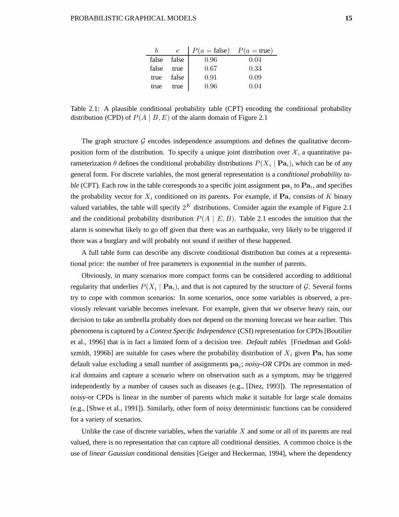
b e P (a = false) P (a = true)false false 0.96 0.04false true 0.67 0.33true false 0.91 0.09true true 0.96 0.04
Table 2.1: A plausible conditional probability table (CPT) encoding the conditional probabilitydistribution (CPD) of P (A | B,E) of the alarm domain of Figure 2.1
The graph structure G encodes independence assumptions and defines the qualitative decom-
position form of the distribution. To specify a unique joint distribution over X , a quantitative pa-
rameterization θ defines the conditional probability distributions P (Xi | Pai), which can be of any
general form. For discrete variables, the most general representation is a conditional probability ta-
ble (CPT). Each row in the table corresponds to a specific joint assignment pai to Pai, and specifies
the probability vector for Xi conditioned on its parents. For example, if Pai consists of K binary
valued variables, the table will specify 2K distributions. Consider again the example of Figure 2.1
and the conditional probability distribution P (A | E,B). Table 2.1 encodes the intuition that the
alarm is somewhat likely to go off given that there was an earthquake, very likely to be triggered if
there was a burglary and will probably not sound if neither of these happened.
A full table form can describe any discrete conditional distribution but comes at a representa-
tional price: the number of free parameters is exponential in the number of parents.
Obviously, in many scenarios more compact forms can be considered according to additional
regularity that underlies P (Xi | Pai), and that is not captured by the structure of G. Several forms
try to cope with common scenarios: In some scenarios, once some variables is observed, a pre-
viously relevant variable becomes irrelevant. For example, given that we observe heavy rain, our
decision to take an umbrella probably does not depend on the morning forecast we hear earlier. This
phenomena is captured by a Context Specific Independence (CSI) representation for CPDs [Boutilier
et al., 1996] that is in fact a limited form of a decision tree. Default tables [Friedman and Gold-
szmidt, 1996b] are suitable for cases where the probability distribution of Xi given Pai has some
default value excluding a small number of assignments pai; noisy-OR CPDs are common in med-
ical domains and capture a scenario where on observation such as a symptom, may be triggered
independently by a number of causes such as diseases (e.g., [Diez, 1993]). The representation of
noisy-or CPDs is linear in the number of parents which make it suitable for large scale domains
(e.g., [Shwe et al., 1991]). Similarly, other form of noisy deterministic functions can be considered
for a variety of scenarios.
Unlike the case of discrete variables, when the variable X and some or all of its parents are real
valued, there is no representation that can capture all conditional densities. A common choice is the
use of linear Gaussian conditional densities [Geiger and Heckerman, 1994], where the dependency

16 PROBABILISTIC GRAPHICAL MODELS
between a variable and its parents is modeled as linear. When all the variables in a network have
linear Gaussian conditional densities, the joint density over X is a multivariate Gaussian [Lauritzen
and Wermuth, 1989]. In many real world domains, such as in neural networks or gene regulation
network models, the dependencies are known to be non-linear. One example is a representation that
models a saturation effect such as a sigmoid CPD (e.g., [Neal, 1992, Saul et al., 1996]).
2.1.4 Inference
A fundamental task in any graphical model is that of inference. That is, we want to be able to
answer general queries of the form P (X | Z) where X,Z ⊂ X , as efficiently as possible. Assume
for example, that we want to evaluate the probability of getting a call from our neighbor P (C) in
the model of Figure 2.1. By the complete probability formula
P (c) =∑
b,e,a,r
P (b, e, a, r, c)
We can improve on this by utilizing the decomposition of the joint probability which results in
P (c) =∑
a
P (c|a)∑
e
P (e)∑
b
P (b)P (a|b, e)∑
r
P (r|e)
which is significantly more efficient. This procedure of variable elimination (summation) is the
basis of all exact inference methods.
Different method designed for batch query processing at the cost of two variable elimination
computations include Bucket Elimination [Dechter, 1996] and Junction Trees (e.g., [Jensen et al.,
1990]), and are widely used in numerous domain. However, these cannot overcome the fact that
inference in Bayesian networks is in general (excluding tree structured networks) NP-hard [Cooper,
1990] (it belongs, in fact, to #P).
Consequently, to cope with large scale networks, a range of approximate inference techniques
have been developed. These include instance or particle based methods such as Gibbs sampling (see
[Neal, 1993] for an overview of inference sampling techniques), variational approximation method
such as the Mean Field approximation (see [Jordan et al., 1998] for an introduction) and Loopy
Belief Propagation (e.g., [Murphy and Weiss, 1999] and references within). While these methods
have shown great success in different scenarios, like exact inference, approximate inference is NP-
hard [Dagum and Luby, 1997] and choosing the best method of inference for a particular task
remains a challenge.

PROBABILISTIC GRAPHICAL MODELS 17
2.2 Learning Parameters with Complete Data
A generative model, such as a probabilistic graphical model, is one that explains, via its inner
constructs and parameters, how the observed data could be generated. As such, when learning a
probabilistic graphical model from data, we want it to faithfully capture the underlying distribution
P ∗ that gave rise to the observations. That is, we want to learn the minimal decomposition structure
G that is an I-map of P ∗ and we want to correctly quantify its parameters. Our ability to do so
is obviously limited by the expressiveness of our model: As discussed above, some generating
distributions cannot be captured faithfully by a Bayesian network, and others cannot be captured by
the formalism of undirected Markov networks. The choice of the conditional probability distribution
representation may also limit our ability to capture P ∗.
In practice, we face an even more fundamental problem: rather than having access to P ∗, or
equivalently to an infinite number of samples generated by it, we are given a finite training set
of samples D = {x[1], . . . ,x[M ]}, that are independently drawn from P ∗. Using the limited
knowledge available to us via D, our goal is to somehow learn a model B = 〈G, θ〉 that best
approximates P ∗. This may require us to take into account particular phenomena that arise in D
and are solely due to its finite nature. In particular, to avoid over-fitting (see below), we may not
want to capture D exactly, either in terms of independence statements that hold in D or in terms of
the parameters of the model learned.
In this section we present the essentials of learning the parameters of a Bayesian network when
the data is complete. That is, we assume that we are given (or have learned) the graph structure G
and structure G and face the problem of learning the conditional probability distribution parameters
θ or the Bayesian network model B. We start with the maximum likelihood approach for learning
parameters and then present a more robust Bayesian approach that typically offers better general-
ization performance. In the next section we present the score based approach to learning structure.
In Section 2.4, we consider both of these tasks in the presence of missing value or hidden variables
and discuss complications that arise in this scenario.
2.2.1 Maximum Likelihood Estimation
The maximum likelihood estimation (MLE) approach is widely used in all fields of learning. At its
core is the intuition that a good model is one that fits the data D well. That is we want to measure
the probability that the model gave rise to the observed data.
Definition 2.2.1: The likelihood function, L(θ : D), is the probability of the independently sampled
instances of D given the parameterization θ
L(θ : D) =
M∏
m=1
P (x[m] | θ) (2.2)

18 PROBABILISTIC GRAPHICAL MODELS
where P (x[m] | θ) is the probability of the m’th complete instance given the parameter of the
network. The log of that function or the the log-likelihood function is
`(θ : D) =
M∑
m=1
log P (x[m] | θ) (2.3)
In the MLE approach, we want to choose parameters θ that maximize the likelihood of the data:
θ = maxθ
L(θ : D) (2.4)
Eq. (2.4) describes optimization in a high dimensional space even for relatively simple network
structures since we need to jointly optimize over the parameters of all the conditional probability
distributions. As in the case of representation and inference, the Bayesian network representation
offers a decomposition of this optimization task. We can use the decomposition property of Eq. (2.1)
to write
L(θ : D) =M∏
m=1
P (x[m] | θ)
=
M∏
m=1
N∏
i=1
P (xi[m] | pai[m] : θXi|Pai)
=N∏
i=1
[M∏
m=1
P (xi[m] | pai[m] : θXi|Pai)
]
=
N∏
i=1
Li(θXi|Pai: D)
where θXi|Paiare the parameters that encode the conditional probability distribution of Xi given its
parents Pai and
Li(θXi|Pai: D) ≡
M∏
m=1
P (xi[m] | pai[m] : θXi|Pai) (2.5)
is the local likelihood function for Xi. Thus, the global optimization problem is decomposed into
significantly smaller problems, where we optimize the parameters of each conditional probability
distribution P (Xi | Pai) independently of the rest.
In the case of full table CPDs the local likelihood can be further decomposed. Suppose we
have a variable Xi with its parents Pai, and a parameter θxi|paifor each possible assignment to
combination of xi and its parents. In Eq. (2.5), different assignments for which Xi = xi and
Pai = pai contribute the same term to the product. Thus, if we group similar assignments and

PROBABILISTIC GRAPHICAL MODELS 19
denote by S[xi,pai] the number of these instances, we can write
Li(θXi|Pa(Xi) : D) =∏
pai
∏
xi
θxi|pai
S[xi,pai] (2.6)
where
S[xi,pai] =∑
m
1 {xi[m] = xi,pai[m] = pai} (2.7)
and 1 {} is the indicator function.
Proposition 2.2.2: The maximal likelihood estimation (MLE) of the parameters of a Bayesian net-
work with multinomial table CPDs is given by:
θxi|pai=
S[xi,pai]∑xi
S[xi,pai](2.8)
The counts S[xi,pai] are the sufficient statistics of the data D. These summarize all relevant infor-
mation from the individual data instances x[1] . . . x[M ] needed for maximum likelihood parameter
estimation of full conditional probability tables. Thus, two different training set may lead to the
same maximum likelihood parameters if their marginal empirical counts S[xi,pai] are the same for
all Xi in the structure. Consequently, optimizing the likelihood function is equivalent to finding the
best approximation for the empirical distribution constrained by the independence assumptions of
G.
2.2.2 Bayesian Estimation
MLE estimation follows the Frequentist approach to statistics that relies solely on the observed data.
This is intuitive since we directly measure the fit of the model to the data. However, in practice when
data is both limited and noisy, this approach can suffer from over-fitting. That is, the model might fit
the data perfectly but have a poor generalization performance on unseen samples. Consider for ex-
ample, learning the parameters of the model in Figure 2.1 (a) from alarm sounding in a typical week
in a suburb of Los Angeles. Even, in earthquake prone California, there is a good chance that we will
have hundreds of burglaries and random alarm sounding and not a single instance of an earthquake.
In this case, using MLE would results in P (alarm=yes | Earthquake=yes) = 0, which ignores our
prior intuition that there is a relation between an earthquake and the chance that the alarm will
sound. Conversely, it could be the case that during that same week a 6.8 earthquake indeed sounded
all the alarms in the area. In this scenario, MLE would set P (alarm=yes | Earthquake=yes) = 1,
which would probably not be realistic for the smaller more common earthquakes.
Therefore, in the (realistic) absence of endless and varied data encompassing all facets of the true
distribution, we would like to learn models that are more robust to fluctuations in the training data

20 PROBABILISTIC GRAPHICAL MODELS
by incorporating prior knowledge into the parameter estimation process. We turn to Bayesian esti-
mation, which formulates this concept of prior belief in a principled manner. The core of Bayesian
estimation is that, prior to seeing the observed data D, we already had some initial prior belief
regarding the domain at hand. The prior belief is encoded by a distribution P (θ). It can be very
informative such as a strong belief that it will not rain in the Sahara on any random day even before
we are actually “observe” the forecast. On the other hand, a uninformative prior can also play an
important role. Consider, for example, a toss of a fair coin. Our prior belief is uninformative in the
sense that we believe that both heads and tails are equally likely. In fact, we belief this so strongly
that seeing 27 heads and 73 tails in a 100 tosses will not really change this belief. In this case we
would like the seemingly uninformative prior belief to constrain MLE that will estimate a probabil-
ity of 0.73 for seeing tails. We would like the prior to help us avoid the bias that is a results of any
finite dataset. (See [Gelman et al., 1995, Pearl, 1988] and reference within for an overview of the
Bayesian formalism and its relation to other approaches.)
Given our prior distribution P (θ) and the observed data D, we “update” our beliefs and use
Bayes rule to compute the posterior distribution
P (θ | D) =P (D | θ)P (θ)
P (D). (2.9)
The term P (D), called the marginal likelihood, averages the probability of the data over all possible
parameter assignments. To estimate a value for the parameters θ that will be used in the prediction
of the (M + 1)th sample, we average over possible values:
θ ≡ P (X[M + 1] | D) =
∫P (X[M + 1] | D, θ)P (θ | D)P (θ)dθ (2.10)
We now address the issue of choosing a convenient prior. When estimating the parameters of
multinomial distributions, the common choice is the use of Dirichlet Priors [DeGroot, 1989]. The
Dirichlet prior distribution for a multinomial variables X is defined by
P (θ) = Dirichlet(α1, . . . αK) ∝∏
j
θjαj−1 (2.11)
where αi are hyper-parameters that correspond to the possible values of X .
In the case of MLE for full Bayesian networks, we have seen that the likelihood function de-
composes according to the networks structure. This allowed us to estimate the parameters θXi|Pai
for each family independently in Eq. (2.4). For Bayesian estimation, we introduce an independence
assumption that will lead to a similar decomposability:

PROBABILISTIC GRAPHICAL MODELS 21
Definition 2.2.3: [Spiegelhalter and Lauritzen, 1990] A parameter prior P (θ) for a Bayesian net-
work is said to satisfy parameter independence if it can be written as
P (θ) =
n∏
i=1
∏
pai
P (θxi|pai)
The decomposition according to the network structure is called global parameter independence.
The further decomposition according to the values pai is called local parameter independence.
Assuming parameter independence, for each multinomial CPD in the network, we can assign an
independent prior distribution θi ∼ Dirichlet(αx1i |pai
, . . . αxKi |pai
). The form of the Dirichlet prior
defined in Eq. (2.11) is surprisingly similar to that of the likelihood in Eq. (2.6). This leads to the
appealing property that Dirichlet is in fact a conjugate prior to the multinomial distribution. That is,
the form of the posterior and prior distributions are similar:
Proposition 2.2.4: If P (θi) is Dirichlet(αx1i |pai
, . . . αxKi |pai
) then the posterior P (θi | D) is
Dirichlet(αx1i |pai
+S[xi1 ,pai], . . . αxKi |pai
+S[xiK ,pai]) where S[xiK ,pai] is the sufficient statis-
tics derived from D.
This important property now allows us, as in the case of Proposition 2.2.2, to compute Eq. (2.10) in
closed form:
Proposition 2.2.5: The Bayesian estimation for the parameters of a Bayesian network with multi-
nomial table CPDs using a Dirichlet prior is given by:
θxi|pai≡ P (Xi[M + 1] = xi | Pai[M + 1] = pai,D) =
αxi|pai+ S[xi,pai]∑
x′iαx′
i|pai+ S[xi′ ,pai]
(2.12)
Thus, the hyper-parameters αxi|paiplay a similar role to the empirical counts and are often referred
to as imaginary counts. M ′ ≡∑
xiαxi|pai
is the imaginary sample size. That is, using a Dirichlet
prior with the above hyper-parameters is equivalent to seeing M ′ samples where the different as-
signment to the variables distribute according to αxi|pai. In order to ensure probabilistic coherence,
the hyper-parameters αxi|paimust satisfy marginalization constraints, in accordance with the net-
work structure. One way to ensure this is to use the BDe prior [Heckerman and Geiger, 1995] to
construct these hyper-parameters. We discuss the details of this prior in details in Section 2.3.1 in a
more general context.
2.3 Structure Learning
In the previous section, we have assumed that the graph structure G is given. In real-life, however,
it is rarely the case that this structure is known and we would like to learn it from data. This task

22 PROBABILISTIC GRAPHICAL MODELS
is not only important from the perspective of gaining a better understanding of the domain but also
has a significant impact on our ability to learn and the quality of the model’s prediction. A missing
edge can cut off important influencing factors while spurious edges leads to many parameters which
in turn lead to over-fitting and a degradation of the generalization capabilities of the model.
There are two basic paradigms for learning the structure of a Bayesian networks. The first
approach is a constraint based approach that uses independence tests directly (e.g., [Spirtes et al.,
1993]): In short, based on some statistical test or oracle, a set of independence statements forms
the constraint set. A network structure to capture this set of constraints to the best extent possible.
Although this approach is intuitive since Bayesian networks are, by definition, independence maps
of the distribution they represent, it suffers from high sensitivity to the statistical test applied. In
this dissertation we adopt the common score based approach. In this framework, we define a score
that measures the compatibility of the model to the data and then search for the best scoring model.
As we will see below, this method is appealing statistically and allows compromises in the choice
of edges at the cost of computational complexity.
The problem of searching for the best scoring structure is essentially a model selection task
and the role of the score is to efficiently guide us towards a beneficial structure. Consequently, all
common scores used in structure learning such as BIC [Schwarz], MDL[Lam and Bacchus, 1994],
BDe [Heckerman et al., 1995a] and BGe [Geiger and Heckerman, 1994] have certain appealing
properties. First, all scores follow Occam’s Razor: if two models achieve the same likelihood then
the simpler one will receive a higher score. The Minimum Description Length (MDL) score [Lam
and Bacchus, 1994], for example, encodes this directly:
ScoreMDL(G : D) = `(θ,G : D)−log M
2Dim(G)−DL(G) (2.13)
where M is the number of instances, Dim(G) is the number of parameters in the model and DL(G)
stands for the description length of G and is the number of bits needed to encode the graph structure.
Second, all scores do not distinguish between independence equivalent models the are probabilisti-
cally indistinguishable (see Definition 2.1.4). Third, given a complete dataset, all scores decompose
according to the network structure and facilitate efficient computation of local structure changes.
This property is crucial (see Section 2.3.3) when learning the structure of large real-life models.
Finally, if G∗ is the generating model, as the number of samples grows to infinity, all scores prefer
G∗ (or an equivalent model) to any other structure.
2.3.1 The Bayesian Dirichlet Equivalent Sample Size Score
The Bayesian Dirichlet equivalent sample size (BDe) or Bayesian score is based on the same prin-
ciples described in Section 2.2: we explicitly represent uncertainty over both the structure and
parameters as a distribution and then combine out prior beliefs P (G) and P (θ | G) to compute a

PROBABILISTIC GRAPHICAL MODELS 23
posterior distribution
ScoreBDe(G : D) = log P (D | G) + log P (G)
where the marginal likelihood P (D | G) averages the probability over all possible parameterizations
of G:
P (D | G) =
∫P (D | G, θ)P (θ | G)dθ
The integration over all possible parameters gives the Bayesian score a bias towards simpler struc-
tures. When the model has many parameters, particularly when the number of sample is small,
there are many different parameterizations for which P (D | G, θ), and consequently the integral
increases. On the other hand, when the probability of the true parameters is peaked (which happens
when the sample size is large), the effect of number of parameters is reduced since P (D | G, θ) is
non-negligible only for few values. Thus the Bayesian score inherently takes care of the problem
of over-fitting a complex model to a small sample size. In fact, it can be shown that, as the num-
ber of samples grows, that the BDe score is equivalent to the Minimum Description Length (MDL)
score [Lam and Bacchus, 1994] that encodes this explicitly, up to an additive constant.
As in the case of parameter, estimation, the choice of priors determines not just the score itself
but also the form that it can take. We require that the prior satisfy the following intuitive property:
Definition 2.3.1: [Heckerman et al., 1995a] A parameter prior satisfies parameter modularity if for
any two graphs G1 and G2, if PaG1i = Pa
G2i then:
P (θXi|Pai| G1) = P (θXi|Pai
| G2)
Priors that satisfy parameter modularity are called factorized priors [Cooper and Herskovits, 1992,
Heckerman et al., 1995a] and facilitate the decomposition of the Bayesian score:
Proposition 2.3.2: If the prior P (θ | G) satisfies global parameter independence and parameter
modularity then
P (D | G) =∏
i
∫
θXi|Pai
∏
m
P (xi[m] | pai[m], θXi|Pai)P (θXi|Pai
)dθXi|Pai
Since P (D | G) already prefers simple structures to complex ones, P (G) is often taken to be uniform
and can thus be omitted from the score. In other cases, it is simply given as input and we assume
here that it can also be decomposed according to the network structure. We can thus decompose the

24 PROBABILISTIC GRAPHICAL MODELS
score into local contributions each depending only on the sufficient statistics of Xi and its parents
ScoreBDe(G : D) =∑
i
FamScoreBDe(Xi,Pai : D) (2.14)
This decomposition plays a crucial rule in Section 2.3.3 and enables us to devise efficient search
algorithms for network structures of high dimension.
Following Section 2.2.2, we use Dirichlet priors for table CPDs. In addition to the simplification
of computation they offer in the case of parameter estimation, they provide a simple closed form
expression for the local family score.
Theorem 2.3.3: [Heckerman et al., 1995a] Let G be a network structure and P (θ | G) be a parameter
prior satisfying parameter independence and parameter modularity. Using full table CPDs and a
Dirichlet prior with hyper-parameters {αxi|pai} then:
FamScoreBDe(Xi,Pai : D) =∑
pai
[log
Γ(αpai)
Γ(αpai+ S[pai])
+∑
xi
logΓ(αxi|pai
+ S[xi,pai])
Γ(αxi|pai)
]
(2.15)
where Γ is the Gamma function and αpai=∑
xiαxi|pai
and S[pai] =∑
xiS[xi,pai]
Proof: The proof outline is interesting in that it emphasizes the Bayesian perspective of computa-
tions. Using the chain rule, the posterior probability of the data can be written as
P (D | G) =
M∏
m=1
P (X[m] | X[1], . . . , X[m− 1],G)
=
n∏
i=1
∏
pai
∏
m:Pai[m]=pai
P (Xi[m] | Xi[1],Pai[1], . . . , Xi[m− 1],Pai[m− 1],G)
where the second line follows from decomposition according to the network structure and rearrange-
ment of terms. We have already taken a Bayesian approach to computing each term in this product
which resulted in Proposition 2.2.5. Using this results along with some algebraic manipulation we
get the desired result.
As noted above, a desired property is that the score reaches its optimum at the true generating
structure. That is, given a sufficiently large number of samples, graph structures that exactly capture
all independencies in the distribution P (are P-maps of P ), will receive a higher score than all other
graphs. This concept is captured in the following definition:
Definition 2.3.4: Assume that the structure of the model generating the observations is G ∗. We say
that our score is consistent if, as M →∞, the following properties hold with probability asymptotic
to 1 (over possible choices of dataset D generated from G∗)

PROBABILISTIC GRAPHICAL MODELS 25
• The structure G∗ will maximize the score
• All structures that are not equivalent to G∗ will have a strictly lower score
Another desired property is that the score be the same for two Bayesian network models that are
independence equivalent. Such a property is called structure equivalence of the score. In order to
achieve structure equivalence, we need to devise a set of hyper-parameters so that our prior will not
bias the score between equivalent structures. This is achieved using a BDe prior [Heckerman and
Geiger, 1995]: we define a probability distribution P ′ over X and an equivalent sample size M ′ for
our set of imaginary samples. The hyper-parameters are then defined to be:
αxi|pai= M ′ · P ′(xi,pai)
Theorem 2.3.5: [Heckerman et al., 1995a] Given complete data, the Bayesian score with BDe prior
is both consistent and structure equivalent.
2.3.2 Scores For Continuous CPDs
Developing a Bayesian score for network with continuous probability distribution is somewhat more
complex. For Gaussian network, the conjugate Normal Wishardt prior (see [DeGroot, 1989]) plays
a similar role to Dirichlet priors in the case of discrete variables. Geiger and Heckerman [1994] use
this prior to develop a closed form Bayesian score called the BGe score. The specifics of this score
are somewhat detailed and we omit these as this score is not used in this thesis.
For general non-linear CPDs, however, there is no simple general form of a Bayesian score.
Thus, it is common to to resort to an approximation of the full Bayesian score that is easy to compute
in the general case, such as the Bayesian Information Criterion (BIC) score [Schwarz]
BIC (D, G) = maxθ
`(D : G, θ)−log M
2Dim[G]
where M is the number of instances in D, and Dim[G] is the number of parameters in G.
2.3.3 Search Algorithm
Given the Bayesian score, or any other commonly used score, learning amounts to finding the
structure G that maximizes the score. Chow and Liu [Chow and Liu, 1968] have shown that learning
the ML tree can be done efficiently using a maximum spanning tree approach [Cormen et al., 1990].
A similar method can be used to learn the maximal scoring tree for any decomposable score. Yet,
despite extensions to particular scenarios (e.g., [Friedman et al., 1997]), learning the structure for a

26 PROBABILISTIC GRAPHICAL MODELS
Algorithm 1: Greedy Hill-Climbing Structure Search for Bayesian Networks
Input : D // training setG0 // initial structure
Output : A final structure G
Gbest← G0
repeatG← Gbest
foreach Add,Delete,Reverse edge in G doG′ ← ApplyOperator(G)if G′ is cyclic then continueif Score(G ′ : D) > Score(Gbest : D) thenGbest← G
′
endend foreach
until Gbest == Greturn Gbest
general Bayesian network, even if the number of parents is limited to two, is NP-hard [Chickering,
1996a].
Thus, we resort to a heuristic greedy search. We define a search space where each state in this
space is a network structure. A set of operators manipulate a network structure to generate a set
of successor states. This defines a graph structure over possible states (networks structures) where
neighboring states are two networks that are one operator away. To perform a search, we start with
some initial structure (usually the empty graph) and apply a greedy search scheme to traverse the
search space in order to locate a high scoring structure.
To facilitate tractable learning, local structure modification operators are considered such as
Add, Delete and Reverse an edge. The decomposability of the score allows us to efficiently evaluate
the benefit such a local structure change. For example, if we add a parent to Xi we need only
recompute the relevant contribution to the score FamScore(Xi,Pai : D). Furthermore, until an
additional parent is added to Xi or an existing parent removed, the contribution of this operator need
not be recomputed.
Even when using local modifications, it is still impossible to traverse the full search space even
for relatively small domains. Thus, we use a local search procedure such as the greedy hill-climbing
algorithm: At each step we evaluate all possible local moves and perform the change that results in
the maximal gain, until we reach a local maximum. The procedure is outlined in Algorithm 1.
The greedy nature of the algorithm is necessary to facilitate learning in practice. However, it is
also means that we our final local maxima model is an inferior one. This problem is a central issue
when learning the structure for practically any real-life domain. Consequently, different methods
are applied to cope with this problem in the discrete search space.
PROBABILISTIC GRAPHICAL MODELS 27
One way to reduce the sensitivity to local maxima is to strengthen the power of the greedy
algorithm at the cost of computational complexity. This can be done by using search algorithm
that are more exhaustive than greedy hill-climbing such as K-best search and time limited Iterative
Deepening (see [Cormen et al., 1990] and reference within for on overview of search procedures).
An appealing alternative that directly confronts the local maxima is that of Tabu search [Glover
and Laguna, 1993]. This method keeps a tabu list record of the last N models visited and rather
than considering only moves that improve the best (local maxima) model, it also considers moves
that improve any of these N models. Tabu search is particularly effective in escaping small local
maxima and plateaus, depending on the size of the tabu list.
A different approach to cope with local maxima is to introduce stochasticity into the search
procedure. The simplest heuristic of this type is to use random restarts when encountering a local
maxima or plateau. At each random restart, several random structural changes are applied to the
best scoring structure, after which the search procedure continues as usual. This approach suffers
from the fact that the “interesting range” of possible random points is typically not known and many
of stochastic go to waste. Despite this, it is often extremely useful in practice. Algorithm 2 outlines
the extension of the basic greedy hill climbing algorithm of Algorithm 1 to include tabu list and
random restarts. This algorithm is the basic search procedure used throughout this dissertation.
Other stochastic methods for escaping local maxima include the bootstrap method [Efron and
Tibshirani, 1993, Friedman et al., 1999b] and various annealing algorithms such as Determinis-
tic Annealing [Rose, 1998] and Simulated Annealing [Kirpatrick et al., 1994]. We discuss these
methods in more details in Chapter 3 where they are particularly relevant.
2.4 Learning with Missing Values and Hidden Variables
In real-life, the observed data is often partial. A patient’s record, for example, will probably never
contain results for all possible tests. Indeed, one of the advantages of probabilistic graphical models
is that, using the ability to perform inference relatively efficiently, we can easily cope with missing
values. An important distinction should be made between observations that are missing at random
(MAR) and observations whose absence influences the domain. For example, the presence or ab-
sence of a biopsy result is clearly not random and is related to the result of a preliminary blood test.
Yet, the vast majority of learning method adopt the MAR assumption without which the learning
problem is practically unapproachable. In this dissertation we adopt the same assumption. We note,
however, that one way to partially cope with observation that are not missing at random is to add
a “MISSING” state for the relevant variables (see [Rubin, 1976] for a discussion of this issue). In
addition to missing values, some of the variables may be hidden or latent. That is, we may never
28 PROBABILISTIC GRAPHICAL MODELS
observe these variables in the data.1 Probably the most common scenario involving a hidden vari-
able is that of clustering, where the class assignment of the objects to be clustered is never observed.
More interestingly, we may want to take the user’s “mood” into account when building a person-
alized web sales engine, but can expect never to observe the actual state of mind of the Internet
surfer.
In this section we give a brief overview of learning in the presence of missing values and hidden
variables. We assume that the hidden variables, if any, are known to exist and their cardinality is
given as input. It is the central goal of the dissertation to explore the significantly harder goal of
learning new hidden variables and their cardinality.
2.4.1 Parameter Estimation
Learning with missing values is significantly harder than learning with complete data since we no
longer have a closed form solution for estimating the parameters of the network. This is a result of
the fact that parameter independence does not necessarily hold and the case of unrestricted multi-
nomial distributions can no longer be decomposed into local estimation problems. Optimization is
consequently in very high dimension. Furthermore, the parameter space typically contains many
local maxima. When some of the variables are hidden (their observation is missing altogether) we
further face the problem of multiplicity of both global and local maxima that arises from possible
permutations of the values of these variables.
The most straightforward approach for parameter estimation with missing values is to use direct
optimization techniques such as gradient ascent and its variants (e.g., [Bishop, 1995]). In the case
of maximum likelihood estimation these methods can also take advantage of the network structure
in some cases (e.g., [Binder et al., 1997]). Unfortunately, optimization if often computationally
demanding due to the large number of parameters and is highly prone to get stuck in inferior local
maxima. In the case of Bayesian estimation, we also face the further complication of optimizing
a poster over the network parameters θ. This is usually infeasible and an approximation must be
used. A common solution is to resort to a Maximum A-Posteriori computation which is similar
to the maximum likelihood case. Alternatively, we can use a sampled (particle) based stochastic
technique that is guaranteed to converge to the true posterior such as Gibbs sampling (e.g., [Neal,
1993]). However, such a method can be extremely slow and can take an impractical amount of time
to achieve reasonable accuracy.
One commonly used alternative is that is used throughout this dissertation is the Expectation
Maximization (EM) algorithm [Dempster et al., 1977, Lauritzen, 1995]. The idea of EM is straight-
forward: since parameter estimation is easy when data is complete, we first “complete” the data
1We note that these variables are MAR by definition. Otherwise, a single “MISSING” value will be observed through-out which will render the distribution of the variable not useful in terms of its ability to effect our prediction abilities.

PROBABILISTIC GRAPHICAL MODELS 29
L(Θ|D
)Θ
L(Θ|D
)
Θ
(a) (b)
Figure 2.4: Illustration of likelihood optimization using: (a) Gradient Ascent that proceeds in thedirection of maximal change; (b) the Expectation Maximization (EM) algorithm that locally ap-proximates the likelihood using a concave function and then optimizes this concave lower-bound.
in the expectation step (E-step) by computing a posterior distribution Q(H | O, θold) of the miss-
ing values H given the observations O and the current model at hand. We can then compute the
expected sufficient statistics by replacing Eq. (2.7) with
IEQ(H|O,θold)[S[xi,pai]] =∑
m
Q(Xi = xi,Pai = pai | o[m], θold) (2.16)
where o[m] is the m’th partially observed instance. These complete sufficient statistics can the be
used to optimize the parameters in the maximization step (M-step) of the algorithm. The resulting
model is then used to repeat the E-step and so on until convergence. It can be shown [Dempster
et al., 1977] that EM is equivalent to lower-bounding the likelihood function at the current model
parameters via a concave function and then taking the maximum of this function as illustrated in
Figure 2.4. Consequently, the EM algorithm is guaranteed to improve the likelihood of the observed
data D at each iteration until convergence to a (typically) local maximum. EM and its variants
(e.g., [Neal and Hinton, 1998]) have proved to be surprisingly effective in practice and are typically
used when the local distribution functions are in the exponential family and sufficient statistics exist.
Generalizations of the EM algorithm using variational methods have also been applied for complex
non-linear conditional probability distributions (e.g., [Saul et al., 1996, Diez, 1993]).
Like gradient methods, the EM algorithm also suffers from the problem of local maxima and
its performance depends on the starting point used. A straightforward method often used to cope
with this is simply to run EM from multiple starting points and choose the best of the local maxima
solution. While there are no guarantees as to the number of random restarts needed for an effective
solution, this method can be surprisingly effective in practice.
2.4.2 Structure Learning
When learning structure in the presence of hidden variables we face further complications. If we
use either the MDL score or the Bayesian score (BDe) then, at each step in the search procedure, we

30 PROBABILISTIC GRAPHICAL MODELS
need to estimate parameters using ones of methods described in the previous section such as the EM
algorithm. Consider, for example, adding the first edge to the starting point empty network. Choos-
ing the best such structure change requires that we consider O(N 2) possible candidate structures.
Without the decomposability assumption that we had in the case of complete data, even evaluating
only the likelihood of each candidate becomes an expensive global optimization procedure. Thus,
in the absence of prior constraints on the network structure, that can significantly reduce the search
space, straightforward structure search is intractable in any interesting domain.
As in the case of parameter learning, a solution that takes advantage of the relative ease of
learning when data is complete is often used. The Structural Expectation Maximization (SEM)
algorithm [Friedman, 1997] generalizes the idea of EM to the scenario of structure learning. The
E-Step is identical to parametric EM where we use the current model to generate the distribution
Q(H | O, θold), thus providing complete sufficient statistics as in Eq. (2.16). In the M-Step we need
to optimize both the structure of the network and its parameters. Given the “completed” dataset
of the E-Step, this is identical in form to structure learning with complete data. It is important to
note that the expected benefit by this approach is significant: rather than re-estimating the model
parameters and expected statistics after each change in structure, the output of a single E-step is
used to perform many structure adaptations (usually until convergence in the search space) often
leading to an order of magnitude and more improvement in running time.
The idea of Structural EM can also be applied for Bayesian learning [Friedman, 1998]. Again,
once the expected sufficient statistics are computed in the E-step, we can proceed as if the data
were complete. Yet, even with this approximating algorithm, Bayesian learning is particularly chal-
lenging in the presence of missing values. Specifically, computation of the marginal likelihood is
intractable and we have to resort to one of several possible approximations [Chickering and Heck-
erman, 1996]. In this dissertation we use the empirically effective and computationally efficient
Cheeseman-Stuts approximation [Cheeseman et al., 1988] for this scenario.

PROBABILISTIC GRAPHICAL MODELS 31
Algorithm 2: Greedy Hill-Climbing Structure Search for Bayesian Networks with Tabu listand random restarts
Input : D // training setG0 // initial structureT SIZE // size of tabu listM EXPAND // maximum number of expansionsM RESTART // maximum number of restartsR MOVES // number of random moves at each restart
Output : A final graph G
Gbest← G0
qLoops← 0eNum← 0while qLoops < M RESTART and eNum < M EXPAND do
// GREEDY with TABUqSteps← 0G← Gbest
while qSteps < T SIZE/2+1 and eNum < M EXPAND doforeach Add,Delete,Reverse edge in G doG′← ApplyOperator(G)if G′ is cyclic or in TABU list then continueeNum← eNum +1if Score(G ′ : D) > Score(Gbest : D) thenGbest← G
′
qSteps← 0
elseqSteps← qSteps +1
endend foreach
end
// RANDOM RESTARTG′ ← ApplyOperator (Gbest,R MOVES)if Score(G ′ : D) > Score(Gbest : D) thenGbest← G
′
qLoops← 0
elseqLoops← qLoops +1
endendreturn Gbest

Chapter 3
Weight Annealing
Training in machine learning is usually posed as an optimization problem : that is, we search for a
hypothesis that maximizes a score on the training data. This is true for regression, classification and
density estimation, as well as most other machine learning problems. (The obvious exception we
are ignoring is pure Bayesian learning, which involves integration instead of optimization, but that
is typically intractable.) Even for straightforward optimization objectives, in interesting hypothesis
spaces like decision trees, neural networks, and graphical models, the problem of finding a globally
optimal hypothesis is usually intractable. This is true whether one is searching for an optimal
combination of hypothesis structure and parameters (e.g., decision tree learning), or just optimizing
the parameters for a given structure (where the likelihood function is optimized). Therefore, most
training algorithms employ local search techniques such as gradient descent or discrete hill climbing
to find locally optimal hypotheses (e.g., [Bishop, 1995]). The drawback is that local maxima are
abundant. Thus, local search often yields poor results. This situation is particularly acute when
learning probabilistic graphical models in the presence of missing data and hidden variables, as
discussed in Section 2.4.
In this chapter we consider annealing like strategies for escaping local maxima. Unlike standard
annealing approaches, we perturb the training data rather than the hypothesis space directly. The
approach is applicable to a wide range of learning scenarios in general, and for learning Bayesian
networks in particular. In Section 3.1, we present a brief background on annealing algorithms.
In Section 3.2 we present the basics of our framework, followed by two perturbation strategies in
Section 3.3. In Section 3.4 we analyze our approach using a toy learning problem. In Section 3.5 we
apply our method to structure search, parameter estimation, and the combined task when learning
Bayesian networks. In Section 3.6, we briefly present an application to an inherently different and
highly non-linear optimization problem. In Section 3.7 we briefly discuss the relation of our method
to other annealing approaches as well as to boosting and bootstrap. We finish with a short discussion
in Section 3.8.
32

WEIGHT ANNEALING 33
Algorithm 3: Generic Annealing Algorithm
Input : D // training seth0 // initial hypothesisτ0 // initial temperature
Output : An hypothesis h
i← 0while τ i > 0 do
1 hi+1 ← Optimize(τ i,hi,D)τ i+1← CoolDown(τ i )i← i + 1
endreturn hi
3.1 Annealing Algorithms
Tabu list and random restarts for discrete structure search, and multiple starting point EM for pa-
rameter estimation were discussed in Chapter 2 as simple and often effective methods for escaping
local maxima. When the optimization problem at hand is difficult, as is often the case for real-life
domains with hidden variables, more sophisticated tools need also be considered. The annealing
family of algorithms are probably the most commonly used tool to avoid local maxima. The basic
idea behind these algorithms is to start by optimizing a related, easy to solve problem and gradu-
ally converge to a solution of the hard problem of interest. Algorithm 3 shows a generic annealing
procedure: At the heart of the algorithm is some cooling policy that starts at a high temperature
τ0 and decreases the temperature τ to 0. The optimization method involved in Line 1 introduces
stochasticity or regularization into the learning process in a magnitude that is a function of the cur-
rent temperature τ i. The algorithm gradually converges on a solution of the original optimization
problem at τ = 0. Below, we briefly present the two most common annealing methods.
The Simulated annealing (SA) algorithm [Kirpatrick et al., 1994] and its variants manipulate
the learning algorithm by allowing “illegal” or score decreasing moves. The algorithm follows a
“propose, evaluate, reject” scheme: a random move is suggested, evaluated, and then accepted if it
improves the score, or with a probability that is proportional to the decrease in score and the current
temperature. The acceptance probability is
P (Accept) =
{1 ∆Score > 0
exp(− 1
τ ∆Score)
otherwise
where ∆Score is the difference in score resulting from the move evaluated, and τ is the current

34 WEIGHT ANNEALING
temperature. At high temperatures, practically any move is allowed while at τ = 0, only score in-
creasing moves are accepted. Simulated annealing is in fact a specific instantiation of the Metropo-
lis procedure [Metropolis et al., 1953], and is thus a Markov Chain process where detailed balance
holds. Thus, Markov chain theory (see for example [Gilks et al., 1996]), guarantees convergence to
the global maximum, if we start at a temperature that is sufficiently high and progress sufficiently
slowly. While this may seem promising, the challenge lies in the choice of an effective cooling
strategy (see [Laarhoven and Aarts, 1987] for an overview of methods). In practice, it is often not
possible to achieve good performance in reasonable time. Simulated annealing has proved bene-
ficial in a variety of optimization tasks such as constraint satisfaction and the traveling salesman
problem.
The Deterministic annealing (DA) algorithm (e.g., [Rose, 1998]) is an annealing approach that
incorporates entropy in the learning objective function, instead of stochasticity in the learning al-
gorithm. As with simulated annealing, the magnitude of the “disturbance” of the true objective is
proportional to the temperature τ . When the system is cooled down, the entropy is lowered until at
τ = 0 the original objective is optimized. In addition, convergence to the global maxima is again
guaranteed in theory, but in practice can be extremely elusive and time consuming. Deterministic
annealing has been used successfully for many problems such as clustering (e.g., [Hofmann and
Buhmann, 1997]).
Somewhat surprisingly, both of these algorithms, which are often considered as state-of-the-art
optimization methods, have not been successful when applied to learning Bayesian networks (see
more details in Section 3.7). It is the goal of this chapter to present a different annealing approach
that is reminiscent of Boosting [Schapire and Singer, 1999] and Bootstrap [Efron and Tibshirani,
1993], and is effective when learning Bayesian networks.
3.2 Weight Annealing
The most common scores used in machine learning are additive on training data, which means that
the score of a hypothesis h on data D = {x[1], ...,x[M ]} is a sum of local scores on each individual
sample, plus an optional regularization penalty
Score(h,D) =∑
m
score(h,x[m]) − penalty(h)
Such scores arise naturally in regression or classification problems, where the local score is typically
the negated prediction error, and in density estimation, where the local score is typically the log
likelihood. Although we will apply our techniques to more general, non-additive scores below, it
will be useful to keep additive scores as a simple example.
At the core of our method is a procedure for reweighting of the training samples to create useful

WEIGHT ANNEALING 35
ascent directions in the hypothesis space. To do this, we augment the score so that it considers a
probability distribution w on the training examples, thus yielding
Score(h,D,w) = M∑
m
wm · score(h,x[m]) − penalty(h) (3.1)
It is first important to understand intuitively how sample reweighting can help to escape local max-
ima. The key idea is that we can cause “informed” changes to be made to the current hypothesis,
rather than arbitrarily alter it. If the hypothesis is poor, then some training samples which contribute
strongly to the score are likely to be outliers that should be down-weighted, whereas other samples
that do not contribute strongly should be up-weighted to reflect their true importance in the under-
lying distribution. That is, a poor hypothesis can fit outliers but under-represent samples that are
actually important. Understanding how the score is influenced by training samples can therefore
suggest plausible perturbations to the data so that superior hypotheses are favored.
Our goal is to perturb the training data to allow the local search algorithm to escape poor local
maxima, under the constraint that we ultimately find a hypothesis that scores well on the original
training distribution. Therefore, the perturbations should not move the training data too far from
their original state, and eventually the data must be restored to its original form to ensure that the
final hypothesis is optimized on the correct distribution. This suggests that we follow an anneal-
ing approach, where we allow the instance weights to change freely early in the search, but then
eventually “cool” the weights towards the original distribution.
Algorithm 4 outlines the generic Weight Annealing (WA) search procedure we suggest, gen-
eralizing on the basic annealing procedure of Algorithm 3. The free parameters in this procedure
are the annealing schedule or cooling policy (Cooldown), the local search method (Optimize), and
the example reweighting scheme (Reweight). For the annealing schedule, we follow a standard ini-
tialization and decay, starting with temperature τ 0 and setting τ i+1 = δτ i, with δ = 0.9, unless
otherwise specified. (Note that this also requires that we set τ to zero once its value numerically
negligble). The optimization procedure depends, naturally, on the learning problem at hand and is
different for learning parameters or learning structure. Note however, that the optimization method
is used as a black box that does not use the temperature parameter. Rather, it is given a weighted
data on which it is applied without any need for modification. Another issue to note is that the local
search can be interleaved with the example reweighting in many ways. For example, one could per-
form full local optimization between each reweighting step, or perform only a partial optimization
between reweightings. We specify the details of how optimization is applied in section Section 3.5.
The final component of our search procedure is the reweighting method. In the next section
we consider two basic techniques for perturbing sample weights to escape local maxima: random
reweighting where weight profiles (vector of weight values for all instances) are randomly sampled,
and adversarial reweighting where the weight profile is updated to explicitly punish the current

36 WEIGHT ANNEALING
Algorithm 4: Weight Annealing Search Procedure
Input : D // training setw0 // initial instance weightsh0 // initial hypothesisτ0 // initial temperature
Output : An hypothesis h
i← 0while τ i > 0 do
wi+1← Reweight(Score,wi,τ i,hi,D)hi+1← Optimize(Score,wi+1,hi,D)τ i+1← CoolDown(τ i )i← i + 1
endreturn hi
hypothesis, with the intent of quickly guiding the search to a more promising solution. In both cases,
as the temperature is lowered, the weight profile is annealed towards the original weights. This
ensures that the search eventually focuses on producing good solutions for the original distribution
of training samples.
Our basic approach has several benefits. First, the perturbation schemes are general and can be
applied to a large variety of hypothesis spaces, either continuous or discrete. Second, our approach
uses unaltered standard search procedures to improve hypotheses at each iteration, rather than em-
ploy the often wasteful “propose, evaluate, reject” cycle of simulated annealing approaches. Third,
because a perturbation of the training data can generate a long chain of search steps in hypothesis
space, a single reweighting step can result in a hypothesis that is very different from the one consid-
ered at the outset (although its score might not be that different). Finally, in the adversarial variant,
the perturbations to the score are not arbitrary. Instead, they force the score to be more attentive to a
subset of the training instances, thus allowing the particular problem at hand to explicitly affect the
annealing procedure.
3.3 Reweighting Strategies
3.3.1 Random Reweighting
The first reweighting approach we consider is a randomized method motivated by iterative local
search methods in combinatorial optimization [Codenotti et al., 1996] and phylogenetic reconstruc-
tion [Nixon, 1999]. Instead of performing random steps in the hypothesis space, we perturb the
score by randomly reweighting each training example. Candidate hypotheses are then evaluated
with respect to the reweighted training set. That is, we use a standard optimization procedure and

WEIGHT ANNEALING 37
a score of the form of Eq. (3.1), with the perturbed weights vector w. After each iteration is com-
plete, we repeat the process by independently sampling new example weights, re-optimizing the
hypothesis, etc., until the magnitude of the weight perturbation is zero.
For convenience, we require the weights to be a probability distribution over the M data in-
stances. To randomly create a vector of weights, we sample from a Dirichlet distribution with
parameter β, so that
P (W = w) ∝∏
m
wβ−1m (3.2)
for legal probability vectors (see, for example [DeGroot, 1989]). When β is large, this distribution
peaks around the uniform distribution. Thus, if we use β = 1/τ i, the randomly chosen distributions
will anneal towards the uniform distribution as τ i decreases with the number of iterations i. At
τ i = 0 we will converge on the original optimization problem. This scheme, that we call Random,
can also be applied to datasets with non-uniform initial weights. To do so, we note that for a
Dirichlet distribution of the form
P (W = w) ∝∏
m
wαmβ−1m (3.3)
the maximum is achieved at
wm =αmβ − 1∑
m′(αm′β − 1)
Thus, if the original weight of sample m is w0m, we choose αm so that
αmβ − 1∑m′(αm′β − 1)
= w0m
for all m. Then, as β grows larger and the distribution peaks around its maximum, each weight will
converge to its original value. Note that the αms are easily computed and that Eq. (3.2) is recovered
if the weights of all instances are equal.
The Random reweighting strategy can be applied to any optimization function problem where
the objective can be expressed as a function of samples and their weights. This make this strategy
applicable to a large number, if not most, learning problems.
3.3.2 Adversarial Reweighting
The second reweighting approach we consider, is to update weights in a way that directly chal-
lenges the current hypothesis. This approach is motivated by the exponential gradient search of
Schuurmans et al. [2001] for constrained optimization problems. We combine their technique with
an annealing process and modify it for a machine learning context. Intuitively, one can challenge a
local maxima by calculating the gradient of the score with respect to the weights and then updating

38 WEIGHT ANNEALING
the weights to decrease the current hypothesis’ score. For example, on a training sample x[m] one
could consider the adversarial weight update
wt+1m ← wt
m − η∂Score(h,D,w)
∂wm
which would explicitly make the current hypothesis appear less favorable and hence less likely to
remain a local maximum. In this way, Score(h,D,w) behaves somewhat like a Lagrangian, in
the sense that the local search attempts to maximize the score over h whereas the weight update
attempts to minimize the score over w, in an adversarial min-max fashion.
This general approach still has to be adapted to our needs. First, we want to anneal the weight
vector towards the original distribution. Therefore we add a penalty for divergence between w t+1
and the original weights w0. We use the Kullback-Leibler measure [Kullback and Leibler, 1951]
to quantify the divergence between these two weight distributions. We heighten the importance
of this term as the temperature is cooled down by using β KL(wt+1‖w0) where β ∝ 1/τ i+1.
Second, to maintain positive weight values, we follow an exponential gradient strategy and derive a
multiplicative update rule in the manner of [Kivinen and Warmuth, 1997]. This adds an additional
penalty term of the KL-divergence between successive weight vectors wt+1 and wt. Combining
these leads to the following penalized score target function
L(h,D,wt+1) = ηScore(h,D,wt+1) + β KL(wt+1‖w0) + γ KL(wt+1‖wt) (3.4)
where 1/β and 1/γ are proportional to the temperature and enforce proximity to the original weights
and the previous weights, respectively.
There are two ways to use this function to derive weight updates. The first is to explicitly min-
imize the penalized score by solving for wt+1 in ∇wt+1L(D, h,wt+1) = 0. If the score function
is convex in w (as is often the case) the solution can be quickly determined by iteration. A second,
more expedient approach, is suggested by Kivinen and Warmuth [1997]: Instead of doing full op-
timization, we heuristically fix the gradient ∇wL to its value at wt and analytically solve for the
minimum of the resulting approximation (up to the step size parameter η). This is tantamount to ap-
proximating the optimal update by taking a fixed step of size η in the exponential gradient direction
from the current weight vector wt.
To derive the update formula, we first have to compute the derivative of L(h,D,wt+1) with
respect to each of the instance weights. Using ∂x log x∂x = log x + 1, we can write
∂KL(wt+1‖w0)
∂wt+1m
=∂∑
m′ wt+1m′ log
wt+1m′
w0m′
∂wt+1m
= logwt+1
m
w0m
+ 1

WEIGHT ANNEALING 39
and similarly for the derivative of KL(wt+1‖wt). Putting these together we get
∂L(h,D,wt+1)
∂wt+1m
= η∂Score(h,D,wt+1)
∂wt+1m
+ (β + γ) log wt+1m − β log w0
m − γ log wtm + C
where C ≡ β + γ is a constant. Fixing ∂Score(h,D,wt+1)
∂wt+1m
to ∂Score∂wm
|wtm
and applying some algebraic
manipulations, we arrive at the multiplicative update form:
wt+1m = αt+1(w0
m)β
β+γ (wtm)
γβ+γ e
− ηβ+γ
“∂Score∂wm
|wt
m
”
(3.5)
where αt+1 is a normalization constant. We refer to scheme as Adversary. We note that in the
update formula ηβ+γ can in fact be written as C · τ · η where C is some constant. Thus, we have a
degree of freedom that results from interchangeability of the temperature τ and the learning rate η.
For convenience, we always use η = 1.
In sum, our second basic reweighting approach is to make adversarial weight updates by fol-
lowing the negative gradient in a well motivated function. This approach can be applied whenever
the original weighted score is differentiable with respect to the weights, for any fixed hypothesis.
Note this is a very weak requirement that is typically satisfied in machine learning scenarios. In
particular, differentiability with respect to the weights has nothing to do with the discreteness or
continuity of the hypotheses—it is a property of how the instance weights affect the score of a fixed
hypothesis. Thus, one could apply the adversarial reweighting approach to decision tree and neural
network training problems without modification.
An important distinction from the Random reweighting approach is noteworthy: randomness is
replaced by a guided methodology where weights are perturbed to minimize an intuitive function.
While random may reach the best solution by chance, as we will see in Section 3.5, the Adever-
sarial approach offers a far better average solution due to its objective dependent guidance. This
distinction also makes the Adversarial approach very different from other annealing approaches
that are oblivious to the current hypothesis in the search procedure.
3.4 Analysis of a Toy problem
As noted in Section 3.1, Markov chain theory (e.g., [Gilks et al., 1996]) guarantees convergence of
the annealing procedure to the global maximum if we start at a sufficiently high temperature and
cool down at a sufficiently slow rate. However, we usually do not have any practical guarantees of
the performance of any annealing method. This is also the case for our Weight Annealing method.
Thus, in this section we analyzed a toy problem to shed some light on situations where we can
expect our method to work, and when we can expect it to fail.
Recall that in Section 3.2 we motivated sample reweighting by the fact that strengthening some

40 WEIGHT ANNEALING
examples and weakening others can transform the hypothesis toward a profitable direction. With this
in mind, we construct a toy example where the direct correspondence between maxima and samples
is made explicit. Consider a training dataset of points D = {x1, . . . , xM}, a set of corresponding
weights W = {w1, . . . , wM}, and the following one-dimensional objective function with a single
free parameter θ
Score(θ,D,w) =∑
i
wi exp
{−
1
2(xi − θ)2
}(3.6)
Note that in this objective, each sample can potentially create a local maxima associated with it and
that is nearby the value of the sample. Figure 3.1(a) shows this objective when the data set consists
of two points x1 = 1 and x2 = 5 with weights w1 = 0.8 and w2 = 0.2, respectively. Also shown
are the three extremum points of the function marked by the dashed vertical lines. Our goal is to
learn the global maximum θ ' x1.
We now want to analyze how the Adversary method will behave given this particular objective.
Setting, for convenience, β = γ = 0.5/τ , the update equation Eq. (3.5) becomes
wt+11 ∝ w1 exp
{−τ exp
{−
1
2(x1 − θ)2
}}
and similarly for wt+12 , both of which are normalized to sum to 1. If the current parameter θ is at the
local maximum near x1, the inner exponent is approximately zero, and wt+11 ∝ w1 exp {−τ}. In
contrast, wt+12 ∝ w2 exp {−τ · c} where c < 1. Consequently, the reweighting step will diminish
w1 and will enhance w2 thus challenging the current hypothesis. Similarly, if the current hypothesis
is in the local maximum near x2, the reweighting step will diminish w2 and enhance w1. Formally,
we can guarantee the following:
Proposition 3.4.1: Let {x1, x2} be two sample points such that |x2 − x1| < ∞, and {w1, w2} be
their corresponding weights. In addition, let x1 < x2 and w1 > w2. Then, using the score defined
in Eq. (3.6), there is a range of temperatures [τl, τh] such that:
1. If θ ' x2 (is at the local maximum nearest to x2) then, for any τ ∈ [τl, τh], after the adver-
sarial reweighting step, the score function will have a single (global) maximum near x1.
2. If θ ' x1 then, for any τ ≤ τh, after the adversarial reweighting step, the score function will
have two maxima near x1 and near x2.
The consequence of the above proposition is that there exists a range of temperature in which, after
adversarial reweighting, using simple gradient ascent optimization will “shift” the parameters in
the direction of the true global maximum. Furthermore, if, after such a shift the temperature is only
lowered, then the parameters will not “escape” to an inferior maximum. If the temperature is further
lowered to zero using any cooling policy, then using simple gradient ascent will converge to the true
global maximum.

WEIGHT ANNEALING 41
0 2 4 60
0.1
0.2
0.3
0.4
0.5
0.6
0.7
0.8
0.9
1OriginalLocal minima
X1 X20 2 4 6
0
0.1
0.2
0.3
0.4
0.5
0.6
0.7
0.8
0.9
1OriginalReweightedLocal minima
X1 X2
(a) τ = 0 (b) τ = 0.5
0 2 4 60
0.1
0.2
0.3
0.4
0.5
0.6
0.7
0.8
0.9
1OriginalReweightedLocal minima
X1 X20 2 4 6
0
0.1
0.2
0.3
0.4
0.5
0.6
0.7
0.8
0.9
1OriginalReweightedLocal minima
X1 X2X1 X20 2 4 6
0
0.1
0.2
0.3
0.4
0.5
0.6
0.7
0.8
0.9
1OriginalReweightedLocal minima
X1 X2
(c) τ = 2.5 (d) τ = 2.5
Figure 3.1: Illustration of adversarial reweighting on a toy problem: Two instances x1 = 1 and x2 =5 are weighted by w1 = 0.8 and w2 = 0.2, respectively. The objective score is
∑i wiexp{−1
2(xi−θ)2} with one free parameter θ. The figures show the score function before (solid blue) and after(dotted red) adversarial reweighting at different temperatures. The dahsed vertical lines mark thelocal minima of the reweighted objective. (a)-(c) shows the change when the current hypothesis(black circle) is at θ0 ' x1. (d) shows the change when the current hypothesis is at θ0 ' x2.

42 WEIGHT ANNEALING
We illustrate the proposition geometrically in Figure 3.1. (a) shows the original objective func-
tion with two local maxima. (b) and (c) show the score function before (solid blue line) and after
(dotted red line) reweighting when the current parameters are near x2 (black circle). When the
temperature is low as in (b), the score function changes a little and there are still two evident lo-
cal maxima after reweighting. When the temperature is sufficiently high as in (c), the reweighting
causes the rightmost maximum to disappear and gradient ascent will push the parameters towards
the true global maximum. (d) shows what happens when the same temperature is used but the
current parameters are near x1. In this case, the leftmost maximum is indeed pushed down but not
sufficiently to erase the local maximum. It can be computed geometrically that for any τ ∈ [2.4, 5.1]
the same phenomena occurs. (A similar geometrical computation can be carried out to prove the
proposition for any x1 and x2.) The above formal guarantee can be extended to some extent
Proposition 3.4.2: Let x1 < x2 < x3 be three distinct points, where |x3 − x1| < ∞, and
{w1, w2, w3} be their corresponding weights. Then, for the score of Eq. (3.6), if it not the case
that w1 < w2 < w3 or w1 > w2 > w3 then there is is a range of temperatures (τl, τh] for which
1. For any τ ∈ (τl, τh], adversarial reweighting followed by gradient ascent will converge to the
parameters of the global maximum regardless of the initial parameter value
2. For any τ ≤ τh, adversarial reweighting followed by gradient ascent will not push the pa-
rameters away from the global maximum
Proof: (Outline) Assume, w.l.g., that w1 > w2, w3 and w2 < w3. Using Proposition 3.4.1, there
is a range [τ 0l , τ0
h ] for which gradient ascent will progress from the parameter at x2 to those at x1
but not the other way around (we loosely use the points here to denote the nearest local maxima).
Similarly, there is a range [τ 1l , τ1
h ] for which it is possible to move from the parameters at x2 to those
at x3 but not the other way around. In addition, there exists such τ 1h so that for any τ > τ 1
h it is
also possible to move from x3 to x2. Using technical manipulations, it can be shown that τ 0h > τ1
h .
From this we can conclude that there is a range (τ 1h , τ0
h ] of temperatures at which it will be possible
to move from x3 to x2 and then to x1 but not the other way around.
It is insightful to understand why the above proposition is guaranteed to work only if the weights
are unordered. If, for example w1 > w2 > w3, then is could be the case that the temperature that
allows the parameters to be pushed from x2 to x1 will also allow it to escape towards x3. At the
same time, it could be that at a cold enough temperature, where escape to x3 will no longer be
possible, a move towards x1 will no longer be possible as well. We can only still guarantee that if
the current parameter is near the global maximum at a low enough temperature, it will stay there.
The above gives us the first clue to where adversary reweighting may fail. In particular, it is not
only the magnitude of the local maxima but also their relative size that influences the behavior of
the algorithm. Another factor that influences the behavior of the algorithm can be the variance of

WEIGHT ANNEALING 43
0 2 4 80
0.1
0.2
0.3
0.4
0.5
0.6
0.7
0.8
0.9
1OriginalLocal minima
X1 X20 2 4 8
0
0.1
0.2
0.3
0.4
0.5
0.6
0.7
0.8
0.9
1OriginalReweightedLocal minima
X1 X20 2 4 8
0
0.1
0.2
0.3
0.4
0.5
0.6
0.7
0.8
0.9
1OriginalReweightedLocal minima
X1 X2X1 X20 2 4 8
0
0.1
0.2
0.3
0.4
0.5
0.6
0.7
0.8
0.9
1OriginalReweightedLocal minima
X1 X2
(a) τ = 0 (b) τ = 2.66 (c) τ = 2.66
Figure 3.2: Illustration of adversarial reweighting on a toy problem: Two instances x1 = 1and x2 = 6 are weighted by w1 = 0.8 and w2 = 0.2, respectively. The objective score is∑
i wiexp{− 12xi
(xi − θ)2} with one free parameter θ. The figures show the score function be-fore (solid blue) and after (dotted red) adversarial reweighting at different temperatures. The dottedvertical lines mark the local minima of the reweighted objective. (a) shows the original “cold” func-tion. (b) shows the change when the current hypothesis (black circle) is at θ0 ' x2 and (c) showsthe change when the current hypothesis is atθ0 ' x1.
each component in the score. Consider, for example, a slightly different score where the variance
of each component is proportional to the value of the corresponding sample
Score(θ,D,w) =∑
i
wi exp
{−
1
2xi(xi − θ)2
}(3.7)
Figure 3.2 illustrates this example. In (b), we can see that there is a temperature τ = 2.66 for which
gradient ascent will not be able to “drift” from the inferior maxima to the global one. (c) shows that
a the same temperature it is already possible to move from the global maximum to the inferior one.
Intuitively, the narrower a component of the score is, the easier it is to overcome its corresponding
maximum. Thus, the algorithm is sensitive not only to the value of the global maximum, but to its
basin of attraction.
The form of the scores of Eq. (3.6) and Eq. (3.7) we use for the toy example was chosen because
of the direct relation between a local maxima and a sample that made some analysis possible. Gen-
eralizing Proposition 3.4.2 to more realistic scores of actual problems that arise in machine learning
remains a theoretical challenge. Another challenge is to understand how our method behave when
multiple local maxima are present. In practice, as we demonstrate in the next sections, adversarial
reweighting performs well on complicated and varied target functions with many local maxima.

44 WEIGHT ANNEALING
3.5 Learning Bayesian Networks
In this section we apply Weight Annealing to three basic tasks of learning Bayesian networks: struc-
ture search, parameter learning in the presence of missing values or hidden variables and the com-
bined challenge of learning both structure and parameters. We finish with evaluation on challenging
real-life data sets.
3.5.1 Perturbing Structure Search
We start by applying Weight Annealing to the problem of learning the structure of Bayesian net-
works with complete data D. To guide the search procedure, we use the decomposable BDe score
(see Section 2.3.1). A crucial property that we utilize when perturbing instance weights is that this
score, like other commonly used scores, is a function of sufficient statistics of the data. For models
in the exponential family, these sufficient statistics have a canonical form as a sum of functions
applied to particular instances. Thus, if S is a sufficient statistic of interest, then
S(D) =∑
m
s(x[m])
where s(x[m]) is a function of a particular training instance. For example, if S(D) counts the
number of times an event occurred in the data, then s(x) is an indicator function that returns 1 if
x satisfies the event, and 0 otherwise. When we perturb the score, we simply need to reweight the
contribution of each instance. Thus, the perturbed statistic is
S(D,w) = M∑
m
wm · s(x[m]) (3.8)
where M is the number of samples and w is a distribution over the training samples. Although the
BDe score itself is not additive, it is nevertheless defined by sufficient statistics of the data and can
therefore be easily adapted to the weighted case.
The BDe score is also differentiable with respect to the weights of the training instances, which
allows us to apply adversarial reweighting. Using Eq. (2.15) we can write the score for the entire
network structure G as
ScoreBDe(G : D) =∑
i
∑
pai
[log
Γ (α(pai))
Γ (S[pai] + α(pai))+∑
xi
logΓ (S[xi,pai] + α(xi,pai))
Γ (α(xi,pai))
]
The only expressions in the score that depend on the weights are the sufficient statistics counts
S[pai] =∑
m wm · P (Pai = pai | em) where em is the evidence of the m’th instance, and
similarly for S[xi,pai]. Using the Digamma function Ψ(x) ≡ Γ′(x)Γ(x) = (log Γ(x))′ [DeGroot,

WEIGHT ANNEALING 45
1989], the derivative of the score with respect to a specific weight wm is given by
∂ScoreBDE(G : D)
∂wm=
∑
i
∑
pai
∑
xi
[Ψ(S[xi,pai] + α(xi,pai))−Ψ(S[pai] + α(pai))
]P (xi,pai | em)
which can readily be evaluated using a numerical approximation to the Digamma function.
Experimental Evaluation
To evaluate the performance of structure learning with weight annealing we start with the synthetic
Alarm network [Beinlich et al., 1989], where we can compare our results to the generating model
that has the additional prior knowledge of the true structure. We compare our methods to a greedy
hill-climbing procedure that is augmented with a TABU-search mechanism and random restarts as
in Algorithm 2 in Section 2.3.3. We use a tabu list of size 200 with 10 random moves at each of the
5 random restarts. This setting allows great flexibility for the learning procedure and is competitive
with state-of-the-art methods. We apply our perturbation methods following the outline specified in
Algorithm 4. We allow the search procedure to fully optimize with respect to the perturbed weights
after each reweighting. When performing Weight Annealing, we limit the tabu list to size 25 and
allow no random restart moves.
It is possible to evaluate the results both in terms of scores on training data and generalization
performance on test data (average log-loss per instance). In all of our experiments the two measures
correlate closely, and therefore we report only test set performance. Figure 3.3 shows the progress
of the test set likelihood during iterations of the perturbed runs. Shown are the average performance
of 100 runs of the Random perturbation method (with the 20%-80% margin in gray) and the Ad-
versary method, compared to the best of random restarts without perturbations, and with similar
running times. Several conclusions are notable. First, both perturbation methods solidly outperform
the random restarts method. In fact, both methods are able to outperform the true structure with
parameters that were estimated using the training data (Silver). Second, the best model overall is
found by Random. However, Adversary is significantly better than Random’s average perfor-
mance. This allows one to either invest a lot of time and achieve a superior model by performing
many random perturbation runs, or obtain a near optimal structure with a single Adversary run.
To emphasize this point, Figure 3.4 shows the cumulative performance of two different setups of
Random (different starting temperatures and cooling factors). The less favorable line has a similar
running time to Adversary. The superior Random takes an order of magnitude longer for each run,
and often reaches what appears to be the achievable global maximum.
We also evaluated the performance of our methods for structure search on a real-life data set.
Stock Data [Boyen et al., 1999] is a dataset that traces the daily change of 20 major US technology

46 WEIGHT ANNEALING
5 10 15 20 25 30 35 40−15.5
−15.4
−15.3
−15.2
Iterations
Like
lihoo
d
Best of random restartsAvg. random reweightingAdversary reweightingSilver Network
Figure 3.3: The progress of test set likelihood (log-loss per instance) during iterations while learningstructure from complete data of the Alarm domain. Compared are the true structure with trainedparameters (Silver), the best of 100 runs of random restarts search without perturbations, 100 runsof the Random perturbation method and a single run of the Adversary method. The gray areamarks the 20%-80% range of 100 Random runs.
stocks for several years (1516 trading days). As shown in Table 3.1, using our Weight Annealing
procedure leads to improvement of the performance of the model on unseen test data.
3.5.2 Perturbing Parametric EM
We now consider the application of the Weight Annealing framework to parameter estimation of
Bayesian networks in the presence of missing data or hidden variables. As discussed in Section 2.4,
this scenario raises many complications including our inability to perform maximum likelihood or
Bayesian estimation in closed form. However, weight perturbation can easily be applied if we use
the Expectation Maximization (EM) algorithm to cope with this scenario. In particular, EM uses
expected sufficient statistics of the data. The perturbed form of these statistics can be obtained by
replacing Eq. (3.8) with
IEQ[S(D,w)] = M∑
m
wm
∑
x[m]
s(x[m],o[m])Q(x[m] | o[m])

WEIGHT ANNEALING 47
−15.35 −15.3 −15.25 −15.2 −15.150
10
20
30
40
50
60
70
80
90
100
Log−loss/instance on test data
Per
cent
at l
east
this
goo
d
Best of random restartsRandom reweighting (fast)Random reweighting (slow)Adversary reweightingSilver network
Figure 3.4: Cumulative performance on test data when learning the structure of the network withcomplete data of the Alarm domain. The x-axis shows test-set likelihood (log loss per instance),the y-axis shows percent of runs that achieve that likelihood or higher. Compared are the true modelwith parameters trained (silver), the best of 100 random runs of the baseline greedy learning method,100 random runs two instantiations of the Random reweighting method, and a single Adversaryreweighting run.
where Q is a posterior distribution over x[m] given the current hypothesis and the partially ob-
served instance o[m]. Note that the above form is a generalization of Eq. (2.16), and enhances the
applicability of the approach to general learning scenarios with missing values or hidden variables.
It is clear that the maximum point of the expected score is not the maximum point of the true
score (for otherwise one iteration suffices to get to the global maximum). Thus, the expected score
is biased. In general, this bias is towards models that are in some sense similar to the one with which
we computed the expected sufficient statistics. This suggests that we do not necessarily want to find
the optimum of the expected score within EM iterations. Instead, we apply a limited number of
EM iterations (e.g., one) within each optimization step of the Weight Annealing procedure shown
in Algorithm 4, and then reweight the instances. The general perturbation scheme is otherwise
unchanged.

48 WEIGHT ANNEALING
−15.3 −15.25 −15.2 −15.15 −15.1 −15.05 −15 −14.950
10
20
30
40
50
60
70
80
90
100
Log−loss/instance on test data
Per
cent
at l
east
this
goo
d
Standard EMRandom reweightingAdversary reweightingGolden Network
−15.1 −15.025 −14.950
10
20
30
40
50
60
70
80
90
100
Log−loss/instance on test data
Per
cent
at l
east
this
goo
d
SEMRandom reweighting SEMAdversary reweighting SEMGolden network
(a) Parametric EM runs (b) Structural EM runs
Figure 3.5: Cumulative learning performance on test data generated from the synthetic Alarm net-work. The x-axis shows test-set likelihood (log loss/instance), the y-axis shows percent of runs thatachieve that likelihood or higher. Compared are 100 runs each of the baseline learning method,computationally intensive Random perturbations and Adversary, as well as the Golden model thatgenerated the training and test instances. (a) Shows results for parameter estimation where fourcentral variables were hidden in the training set and true structure is used. (b) Shows results forestimation of the parameters as well as the structure from the same dataset.
Experimental Evaluation
We examine our method on the synthetic Alarm network. Figure 3.5(a) compares 100 random runs
of standard parametric EM, computationally intensive Random perturbation, and an Adversary
run. Because of the limited number of EM iterations, Adversary takes only about 15 times longer
than a single parametric EM run, and Random takes around 50 times longer than a single EM run.
We can clearly see the advantage of the Adversary method, which achieves what appears to be the
attainable global maximum using the finite training set. This maximum is reached by only a few of
the random EM and Random perturbation runs, and is not far from the true structure and parameters
(Golden) that generated the test data.
3.5.3 Perturbing Structural EM
The final and most difficult task we explore for Bayesian networks is that of learning both the
parameters and the structure of the model. As in the case of parameter estimation, the use of the
Structural EM (SEM) approach [Friedman, 1997, 1998] facilitates the use of Weight Annealing:
Like EM, the algorithm is based on expected sufficient statistics that can be readily perturbed.

WEIGHT ANNEALING 49
Experimental Evaluation
The setting is identical to the one used in the EM runs, but we also attempt to learn the topology
of the network. The starting point of the search is a structure where all the hidden variables are
parents of all the observed nodes. Figure 3.5(b) shows cumulative results for 100 random runs for
the synthetic Alarm example. The Structural EM runs have a very low variance and are worse
than over 90% of the Random perturbation runs. As with parametric EM, but more markedly,
the Adversary method dominates random reweighting. Note that it halves the distance from the
baseline performance to the performance of the true network.
3.5.4 Evaluation of real-life domains
To conclude the evaluation of Weight Annealing for learning Bayesian networks, we consider a
number of real-life datasets where we learn both the structure and parameters.
• The Soybean [Michalski and Chilausky, 1980] disease database from the UCI machine learn-
ing repository contains 35 variables relevant for the diagnosis of 19 possible plant diseases.
There are 307 training instances and 376 test instances, with many missing values.
• The Audiology data set [Bareiss and Porter, 1987] from the UCI machine learning repository,
contains 69 variables relevant to illnesses relating to audiology disfunctions. There are only
202 training instances an 26 test instances with numerous missing values.
• Rosetta’s compendium [Hughes et al., 2000] consists of gene expression data of 6000 Sac-
charomyces cerevisiae genes (variables) and 300 experiments (samples). We used the pre-
processing of Pe’er et al. [2001] to discretize the data and concentrated on 37 genes which
participate in the stationary phase stress response that they identify.
For each data set we performed 5-fold cross validation and compared the log-loss performance on
independent test data. Table 3.1 summarizes the results. Shown are results for best of random
restarts Structural EM runs, average and 80% values of Random perturbation runs, and the Adver-
sary method. Both perturbation methods achieve superior results to random restarts Structural EM.
Similar to what was observed in structure search, it is sometimes possible to reach a superior model
to Adversary by performing many Random perturbation runs.
In all domains, the perturbation methods improves over the baseline. For the challenging prob-
lem of learning structure in the presence of hidden variables this improvement is quite significant.
For the Soybean dataset, for example, an average improvement of 0.19 bits per instance over a
test set with 376 test instances, means that the unseen samples are more then 274 more likely given
the model learned by the adversarial perturbation method, relative to the best of state-of-the-art
Structural EM runs with Tabu list and random restarts.

50 WEIGHT ANNEALING
Table 3.1: Summary of results on independent test data for several data sets for the structure searchand structural EM problems. Shown are log-loss per instance of improvement in performance withrespect to the best of the random restarts baseline. Compared are the mean of the Random pertur-bation method (along with the 80% mark) and the Adversary method.
Domain Random 80% AdversarySearch Stock −0.02 +0.01 +0.03
Alarm +0.15 +0.18 +0.17
SEM Rosetta −0.05 +0.27 +0.09Audio +0.00 +0.39 +0.23Soybean +0.19 +0.32 +0.19Alarm +0.25 +0.31 +0.33
3.6 Learning Sequence Motifs
All of our case studies so far have addressed unsupervised density estimation problems in the form
of learning Bayesian networks. To demonstrate the wide range applicability of Weight Annealing,
we now examine a completely different discriminative learning scenario. The problem is to perform
non-linear logistic regression in order to find regulatory motifs in DNA promoter sequences; i.e., ,
short subsequences that regulate the expression of genes. In particular, a motif is defined as a
relatively short signature of about 8-20 nucleotides (DNA letters) that appears somewhere in the
DNA sequence—the exact location of which is unknown and can vary from sequence to sequence.
An example of a motif might be the sequence ACGCGT. Unfortunately, most known motifs are not
preserved perfectly in the DNA, and one generally has to allow for substitutions in one or several
positions. Accordingly, the common representation of a motif is as a weight matrix [Durbin et al.,
1998] which describes the weight of each of the four possible DNA letters for each position within
the motif. Intuitively, a subsequence that has a large sum of letter weights is said to match the motif.
We use the notation wi[x] to denote the weight of the letter x in the i’th position.
Following Barash et al. [2001] and Segal et al. [2002], we define the basic training problem in
discriminative terms. Given N promoter sequences s1, . . . , sN , where the n’th sequence consists
of K letters sn,1 . . . , sn,K , and a set of of training labels l1, . . . , lN , where li is 1 if the sequence
is regulated by the motif and 0 if it is not (these labels can be obtained from different biological
experiments), we wish to maximize the log-loss∑
i P (ln | sn) where
P (ln = 1 | Sn,1, . . . , Sn,K) = logistic
log
v
K
∑
j
exp{∑
i
wi[Sn,i+j]}
and logistic(x) = 11+e−x is the logistic function and v is a threshold parameter. Segal et al. [2002]
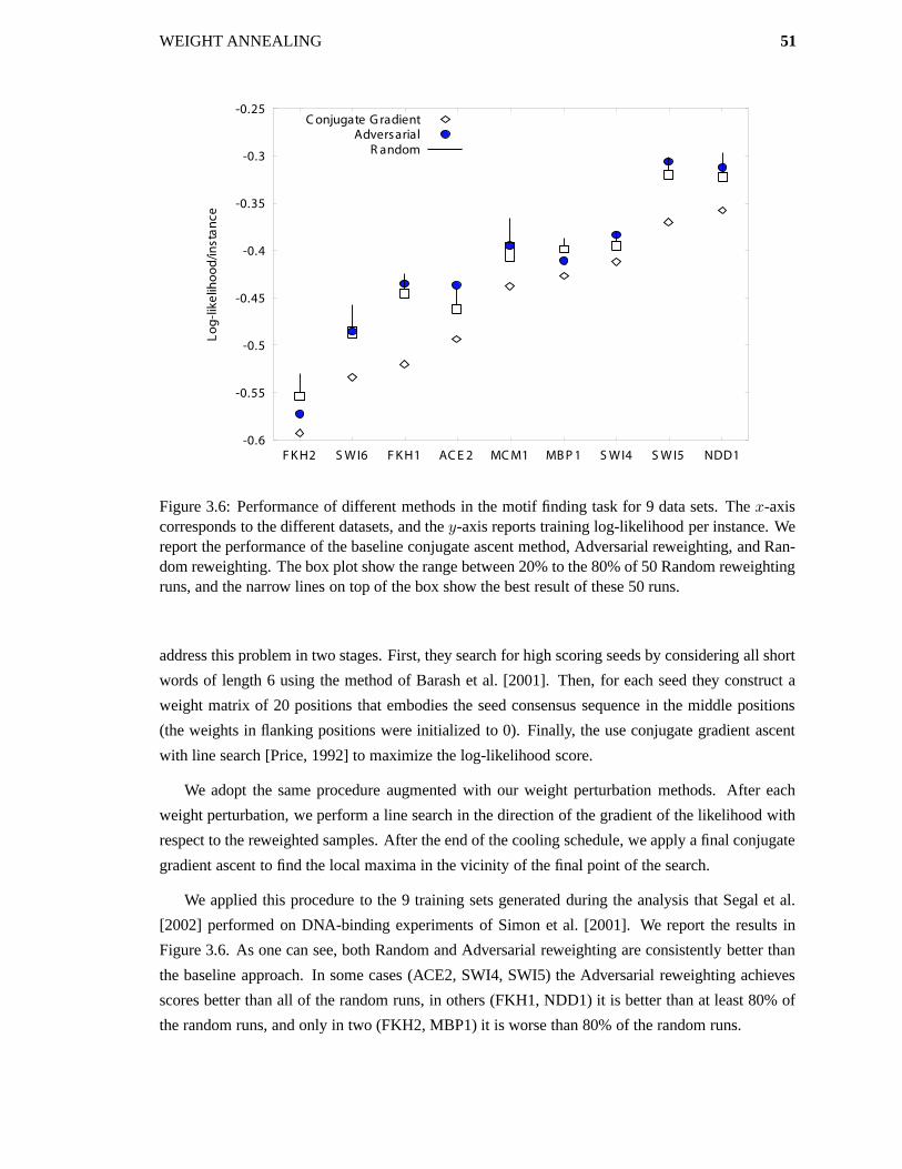
WEIGHT ANNEALING 51
-0.6
-0.55
-0.5
-0.45
-0.4
-0.35
-0.3
-0.25
Lo
g-l
ike
liho
od
/in
sta
nc
e
C onjugate G radientAdversarial
R andom
AC E 2F K H1F K H2 MB P 1MC M1 NDD1S W I4 S W I5S W I6
Figure 3.6: Performance of different methods in the motif finding task for 9 data sets. The x-axiscorresponds to the different datasets, and the y-axis reports training log-likelihood per instance. Wereport the performance of the baseline conjugate ascent method, Adversarial reweighting, and Ran-dom reweighting. The box plot show the range between 20% to the 80% of 50 Random reweightingruns, and the narrow lines on top of the box show the best result of these 50 runs.
address this problem in two stages. First, they search for high scoring seeds by considering all short
words of length 6 using the method of Barash et al. [2001]. Then, for each seed they construct a
weight matrix of 20 positions that embodies the seed consensus sequence in the middle positions
(the weights in flanking positions were initialized to 0). Finally, the use conjugate gradient ascent
with line search [Price, 1992] to maximize the log-likelihood score.
We adopt the same procedure augmented with our weight perturbation methods. After each
weight perturbation, we perform a line search in the direction of the gradient of the likelihood with
respect to the reweighted samples. After the end of the cooling schedule, we apply a final conjugate
gradient ascent to find the local maxima in the vicinity of the final point of the search.
We applied this procedure to the 9 training sets generated during the analysis that Segal et al.
[2002] performed on DNA-binding experiments of Simon et al. [2001]. We report the results in
Figure 3.6. As one can see, both Random and Adversarial reweighting are consistently better than
the baseline approach. In some cases (ACE2, SWI4, SWI5) the Adversarial reweighting achieves
scores better than all of the random runs, in others (FKH1, NDD1) it is better than at least 80% of
the random runs, and only in two (FKH2, MBP1) it is worse than 80% of the random runs.

52 WEIGHT ANNEALING
3.7 Relation to Other Methods
Annealing Algorithms
Both our reweighting strategies share the generic annealing framework outlined in Algorithm 3.
Several differences from the standard algorithms are worth noting: Our method changes the op-
timization space of the learning procedure by perturbing the goal functional. Simulated Anneal-
ing [Kirpatrick et al., 1994], on the other hand, changes the “rules of the game” by allowing moves
that decrease the score with proportion to the current temperature. This approach is often extremely
effective when a small number of score decreasing moves is needed to escape an inferior local
maxima. However, the approach suffers from two main drawbacks: First, the perturbation is inde-
pendent from both the problem and the hypothesis in contrast to the guided adversarial reweighting
method. Second, the “propose, evaluate, reject” cycle is often wasteful. This is particularly true
if the evaluation of candidate hypothesis is costly, as is the case when evaluating the benefit of
Bayesian network structures. We have applied simulated annealing as described by Heckerman
et al. [1995a] for all the experiments in the previous sections. However, using a range of parameters
(around those they suggest), we get significantly worse results than the baseline search method. This
is consistent with the results of Chickering [1996b], who demonstrated that using multiple restarts
greedy hill-climbing is more effective than simulated annealing when learning Bayesian networks.
Deterministic Annealing [Rose, 1998] is even more closely related to our method. Like our ap-
proach, it uses a black-box optimizer and applies it to a perturbed problem. The perturbation of the
score is done by explicitly introducing entropy into the objective in a magnitude that is proportional
to the current temperature. This added component serves as a smoothing factor of the landscape
to be optimized. Somewhat surprisingly, despite success in other tasks such as classification, ap-
plication of Deterministic Annealing for learning Bayesian network Ueda and Nakano [1998] have
not been promising. In particular, Whiley and Titterington [2002] have demonstrated why learning
Bayesian networks with hidden variables using Deterministic Annealing is problematic. Finally,
despite the obvious similarity between our objective function and that of Deterministic Annealing,
the rationale for the scores used in the two cases is quite different. It is unclear if there are deeper
connections between the two methods.
Boosting
There are interesting relationships between the adversarial reweighting and ensemble learning meth-
ods such as boosting [Schapire and Singer, 1999]. Both methods share the central idea that at each
step the weights of the samples that are not predicted well by the current hypothesis are amplified.
However, there are some fundamental differences. On an intuitive level, both methods are inherently
different in the motivation for this reweighting. In the case of boosting, the goal is to concentrate on
the hard samples. In the case of adversarial reweighting, the goal is to challenge the current hypoth-
esis and put its robustness to a test. Another difference is that boosting attempts to build a weighted

WEIGHT ANNEALING 53
ensemble of hypotheses that achieves a good score, whereas we are deliberately seeking a single
hypothesis. On a technical level, boosting derives its weight updates by differentiating the loss of
an entire ensemble [Mason et al., 2000], whereas our weight updates are derived by taking only the
derivative of the score of the most recent hypothesis. Interestingly, although we do not exploit a
large ensemble, we find that our method still produces hypotheses that generalize well to unseen
test data. Although initially surprising, this phenomenon is explained by the fact that adversarial
reweighting of samples discovers hypotheses that obtain good scores while simultaneously being
robust against perturbations of the training data, which confers obvious generalization benefits.
Bootstrap
Our method is also reminiscent of the Bootstrap approach of Efron and Tibshirani [1993]. Bootstrap
is a statistically motivated approach that can be used to provide confidence measures for features of
Bayesian networks learned from data [Friedman et al., 1999b]. In short, this approach uses several
random re-samplings of the data to learn different networks. Confidence measures from these net-
works can then be used to learn more robust models bypassing some of the local maxima that are
a result of problematic noise in the data. Although both methods manipulate a black-box optimiza-
tion procedure by effectively altering the weights of instances, there are several inherent differences.
Rather than using an annealing procedure, the bootstrap approach learns many models from inde-
pendent datasets that are sampled from the original training data. This re-sampling procedure is
oblivious to the target function as well as to the performance of the hypothesis. Furthermore, in-
stead of a single hypothesis that is a local maximum of the original problem, the bootstrap approach
generates an ensemble of hypotheses, each optimizing a different and slightly perturbed problem.
These need to be merged into a single hypothesis using several possible approaches (e.g., [Friedman
et al., 1999b]).
3.8 Discussion
In this chapter we presented a general, annealing like, method for escaping local maxima. The
essence of our Weight Annealing (WA) approach is to perturb the relative weight of the training
instances in a gradually diminishing magnitude. Thus, we perturb the target function rather than
the optimization procedure, and look for optimal solutions of the perturbed problem. As we have
shown, such perturbations allow one to overcome local maxima in several learning scenarios. On
both synthetic and real-life data, our approach seems to lead to significantly improved models when
learning the structure of Bayesian networks with complete data, learning parameters with missing
data, and learning both parameters and structure. The improvements are particularly impressive for
the complex problem of learning both structure and parameters with hidden variables, where the
problem of local maxima is acute.
The perturbation of instance weights is particularly attractive in its applicability for a wide range
54 WEIGHT ANNEALING
of learning problems. It is not only easy to find reweighted versions of standard learning scores, but
sample weights are also easily incorporated into non-trivial learning procedures such as EM. In
doing so, one can exploit the expected sufficient statistics for efficient search, and then perturb the
expected score to find models that have a better score. We compared two strategies for generating the
sequences of weights during annealing: randomized reweighting and adversarial reweighting. Our
results show that both approaches dominate the straw-man of multiple restart search. Randomized
reweighting can sometimes achieve better performance, but this might require performing several
annealing runs. The deterministic adversarial strategy has the advantage of achieving comparable
performance in a single run.
The random reweighting approach we introduced has also been applied in Friedman et al. [2002]
as well as Barash and Friedman [2002] for learning phylogenetic trees and context-specific cluster-
ing models, respectively. Both papers report significant improvements when using Weight Anneal-
ing.
One avenue that we did not explore is the combination of a randomized element within the de-
terministic adversarial strategy. It is also clear that for realistic applications, we need to tune the
implementation to reduce the number of iterations. This can be done by incorporating more so-
phisticated cooling strategies from the simulated annealing literature (e.g., [Laarhoven and Aarts,
1987]) or the deterministic annealing literature (e.g., [Rose, 1998]). It is also worth exploring im-
proved ways to interleave the maximization and the reweighting steps. This may lead to significant
improvement in performance, possibly at a marginal computational cost. Finally, the empirical
success of these methods raises the challenge of providing a better theoretical understanding of
their effectiveness. This is particularly intriguing for the adversarial reweighting strategy that has
similarities to boosting and multiplicative update strategies. Despite the interchangeability of the
temperature and the learning rate, the analysis of these methods does not seem to directly apply to
our setting.

Chapter 4
Discovering Hidden Variables: A
Structure-Based Approach
Our main goal in this dissertation is to learn new hidden variables. This involves determining the
existence of a variable, inserting it effectively into the network structure, and setting its cardinality
in the case of discrete variables. Obviously, all these tasks add significant difficulties to the already
complex problem of learning in the presence of hidden variables, when they are known to exists.
In Chapter 1, we qualitatively discussed why hidden variables should not be ignored: In theory, we
can still construct a network that captures all the dependencies in the marginal distribution over the
observed variables. However, as we illustrated in Figure 1.1 for the cancer domain, this can result in
a model that is less desirable in terms of representation, as it contains significantly more parameters
and edges than the succinct model with the hidden variable.
When a hidden variable is known to exist, we can introduce it into the network and apply
known Bayesian networks learning algorithms. If the network structure is known, algorithms such
as EM [Dempster et al., 1977, Lauritzen, 1995] or gradient ascent [Binder et al., 1997] can be used
to learn parameters. If the structure is not known, the Structural EM (SEM) algorithm of [Friedman,
1998] can be used to perform structure learning with missing data. However, we cannot simply
introduce a “floating” hidden variable and expect the search algorithm to place it correctly. In fact,
if the hidden variable is placed where it does not improve the likelihood of the model, there is a good
chance it will be disconnected by the local search algorithm, after which it will never be worthwhile
to reconnect it to the network structure. Thus, in applying these algorithms we implicitly assume
that some other mechanism introduces the hidden variable in approximately the right location in the
network structure. Our goal in this chapter is then to answer the following two questions:
• Should we introduced a new hidden variable into the network structure?
• Where should we initially place it within the network structure?
55

56 DISCOVERING HIDDEN VARIABLES: A STRUCTURE-BASED APPROACH
H
Children of H
Parents of H
H
Children of H
Parents of H
Clique over children of H
Parents of H
all parents connected to all children
Clique over children of H
Parents of H
all parents connected to all children
(a) Original network (b) After removal of H
Figure 4.1: Schematic illustration of Proposition 4.1.1. (a) shows a network fragment where ahidden variable H separates between some of its parents and children. (b) shows the resultingnetwork fragment when H is not included in the structure and we require that no new independenceassumptions are introduced into the network structure.
(We defer the task of learning the cardinality of the hidden variable to Chapter 5.) We investigate
what is arguably the most straightforward approach for inducing the existence of a hidden variable.
We formally show that the phenomena demonstrated in Figure 1.1, and briefly mentioned in Heck-
erman [1998], is a typical effect whenever a hidden variable is removed from the network structure.
Based on this fact, our approach tries to reverse engineer this phenomena to suggest new hidden
variables, and is roughly as follows: We begin by using a standard Bayesian network model se-
lection algorithm to learn a structure over the observed variables. We then search the structure for
substructures, which we call semi-cliques, that are potentially induced by a hidden variable. We
temporarily introduce the hidden variable in a way that alters the sub-structure, and then continue
learning based on that new structure. If the resulting structure improves the score, we keep the hid-
den variable. Surprisingly, this basic technique does not seem to have been pursued. We provide a
concrete and efficient instantiation of this approach and show how to integrate it with existing learn-
ing algorithms such as the Structural EM algorithm. We apply our approach to several synthetic
and real-life datasets, and show that it often provides a good initial placement for the new hidden
variable. We can therefore use it as a preprocessing step for Structural EM, substantially reducing
the search space of the algorithm.

DISCOVERING HIDDEN VARIABLES: A STRUCTURE-BASED APPROACH 57
4.1 Detecting Hidden Variables
In the example of Figure 1.1 discussed above and that motivates our approach, the hidden variable
“Cancer” is the keystone for the conditional independence assumptions in the network. Without it,
many of the independencies of Figure 1.1(a) simply do not hold. As a consequence, the marginal
distribution over the remaining variables has almost no structure and includes many edges, creating
an undesirable representation. We can show that this phenomena is a typical effect of removing a
hidden variables:
Proposition 4.1.1: (see Figure 4.1 for illustration)
Let G be a network over the variables X = {X1, . . . , XN},H . Let I be the conditional indepen-
dence statements — statements of the form Ind(X ⊥ Y | Z) — that are implied by G and do not
involve H . Let G ′ be the graph over X1, . . . , XN that contains an edge from Xi to Xj whenever G
contains such an edge, and in addition: G ′ contains a clique over the children of H , and G ′ contains
an edge from any parent of H to any child of H . Then, there exists a distribution P (X ,H) such
that G is an I-map of P (X ,H) and G ′ is a minimal I-map of P (X ) =∑
h P (X ,H).
Proof: To prove that G ′ is an I-map, we need to show that the independence statements encoded in
G′ indeed hold in P (X ). To show that it is a minimal I-map we need to prove that removing any
edge from G ′, renders it a non-I-map of P (X ).
We start with the latter task. Clearly, any edge Xi → Xj in the original network G must also
be included in G ′, since the existence of such an edge means that in P (X ,H) (of which G is an
I-map), Xi and Xj may be dependent, even when conditioned on all other variables. Thus, only
the edges we added in the construction of G ′ may be suspected as being redundant. Consider an
edge Pi → Cj , from some a parent Pi of H to some child Cj of H . In the original structure there
existed a path Pi → H → Cj . To render Pi and Cj independent this path (and possibly others)
must be blocked (see discussion of d-separation in Section 2.1.1). This only occurs if H is observed.
Thus, when H is not included in the model, we cannot guarantee that these two variables are not
dependent making the edge Pi ← Cj necessary to ensure I-mapness of G ′ with respect to P (X ).
Similarly, consider the path Ci ← H → Cj between two children of H . The original structure G
implies that unless H is observed, Ci and Cj cannot be declared independent. Thus, either Ci → Cj
or Ci ← Cj is requires. This holds for any two children of H in the original structure.
We now show that the independencies encoded in G ′ hold in P (X ). Obviously we need only
consider independencies that were added as a result of the removal of H . The removal of H from the
structure can only effect independencies of variables if H lies in some path between these variables.
All such paths must pass either through parents of H , its children, or both. If H is at the bottom of
a v-structure Pi → H ← Pj along this path, it blocks the dependency since it is unobserved. This
only adds dependencies to those encoded in G and does not effect I-mapness. If H lies along the
path so that Pi → H → Cj , the removal of H can introduce a new independency between Pi and

58 DISCOVERING HIDDEN VARIABLES: A STRUCTURE-BASED APPROACH
(a) (b)
Figure 4.2: (a) A semi clique that is missed by our algorithm and is composed of two 5-cliques thatare relatively sparsely connected. (b) A 4-clique structure with one edge missing. This is a slightlyrelaxed version of a semi-clique, that is still accepted by our algorithm.
Cj (or ancestors of Pi and descendants of Cj). However, the edge Pi → Cj directly cancels this
potential independence (which is exactly why it was required for minimality). A similar argument
for the case of a path that passes through Ci ← H → Cj , shows that no new independencies are
introduced in G ′, and thus it is an I-map of P (X ).
Our strategy is to define an approach that will suggest candidate hidden variables by finding
structures characterized by the above proposition in the context of a learning algorithm. That is, we
will first learn a network using a standard structure learning algorithm, and then look for substruc-
tures that are potentially a results of a missing hidden variable. In practice, it is unreasonable to
hope that there is an exact mapping between substructures that have the form described in Propo-
sition 4.1.1 and hidden variables: Learned networks are rarely an exact reflection of the minimal
I-map for the underlying distribution. We therefore use a somewhat more flexible definition, which
allows us to detect potential hidden variables:
Definition 4.1.2: A semi-clique is a set of nodes S where each node X ∈ S is linked to more than
more than half of the nodes in S. That is,
|AdjGX(S)| >1
2|S|
where |S| is the number of elements in the set S and AdjGX(S) are the adjacent nodes (neighbors)
of X in the graph G that are in the set S.
We propose a simple heuristic for finding semi-cliques in the graph. We first observe that each
slightly stricter version of a semi-clique must contain a seed which is easy to spot; this seed is a
3-vertex clique.

DISCOVERING HIDDEN VARIABLES: A STRUCTURE-BASED APPROACH 59
Algorithm 5: FindHidden
Input : G // a network structureOutput : A list of candidate children sets (semi-cliques) for hidden variables in G
CliqueList← empty listSeedList← all 3-cliques in G
foreach seed in SeedList doclique← ExpandClique(seed,G )if size(clique ) > MIN CLIQUE SIZE then
Insert clique into CliqueListend if
end foreachreturn CliqueList
Procedure: ExpandClique
Input : seed // a list of variablesG // a network structure
Output : A semi-clique expanded from seed
SemiClique← seed
repeatforeach variable X not in SemiClique do
if IsSemiClique(SemiClique∪X) thenSemiClique← SemiClique ∪X
end ifend foreach
until SemiClique not expandedreturn SemiClique

60 DISCOVERING HIDDEN VARIABLES: A STRUCTURE-BASED APPROACH
Proposition 4.1.3: A set S of N nodes where each node has more than bN2 c, must contain a full
clique of size 3.
Proof: Consider a semi-clique S with N nodes, and let Xi be an arbitrary node in it. Xi must have
at least bN2 + 1c neighbors in the semi-clique. Let Xj be one of Xi’s neighbors (adjacent nodes).
Xj must also have at least bN2 +1c neighbors in the semi-clique. But there are at most N−bN
2 +1c
nodes that are not neighbors of i. Hence, AdjGXi(S) and AdjGXj
(S) cannot be disjoint. Any node
in the intersection, together with Xi and Xj , forms the required 3-clique.
The first phase of the algorithm is outlined in Algorithm 5: It is starts with an exhaustive search
for all 3-cliques in the graph (by definition all of these are also semi-cliques). The algorithm then
tries to expand each of them into a maximal semi-clique in a greedy way using the procedure Ex-
pandClique. At each iteration this procedure attempts to add a node to the “current” semi-clique.
If the expanded set satisfies the semi-clique property, then it is set as the new current semi-clique.
These tests are repeated until no additional variable can be added to the semi-clique. The algorithm
outputs the expansions found based on the different 3-clique “seeds”. We note that this greedy
procedure does not find all semi-cliques. The exceptions are typically two semi-cliques that are
joined by a small number of edges, making a larger legal semi-clique. These cases, an example of
which is illustrated in Figure 4.2(a), are of less interest because they are less likely to arise from
the marginalization of a hidden variable. In practice, we allow a little leeway when searching for
semi cliques, also accepting structures where each node is connected to exactly half of the other
nodes. This allow us to captures structures such as a 4-clique with just one edge missing as shown
in Figure 4.2(b).
In the second phase, we convert each of the semi-cliques to a structure candidate containing a
new hidden node, reverse engineering the phenomena of Proposition 4.1.1. Suppose S is a semi-
clique so that we suspect all of the variables in Q may be the children of an unknown hidden variable
H . We introduce such an H into the network structure and (ensuring acyclicity)
• make H the parent of all variables in S
• remove all edges between the variables in S
• replace each edge Pi → Sj , from some parent Pi (that is not in S) to a child Sj by Pi → H .
This process results in the removal of all intra-clique edges and makes H a proxy for all “outside”
influences on the nodes in the semi-clique S.
Our goal is to provide an efficient and effective starting point for the structure learning algorithm
that will follow the introduction of a new hidden variables into the network structure. Thus, it is
useful to analyze the complexity of our algorithm. The first stage finds all the 3-cliques in the graph.
This is done using a greedy algorithm that examines all possible pairs of parents and children for

DISCOVERING HIDDEN VARIABLES: A STRUCTURE-BASED APPROACH 61
each node. In theory, for a network with n nodes this stage requires the enumeration of the O(N 3)
possibilities. In practice, however, since the number of parents and children in a typical network can
be bounded by a small constant, the complexity is almost linear in the number of nodes. Next, we
try to expand each 3-clique by gradually adding related variables from the network. If the network
is represented efficiently, checking the neighborhood criterion is linear in the size of our current
semi-clique. The algorithm can, in principle, require N 2 iterations before convergence; in practice,
the number of iterations is linear in the size of the semi-clique. Thus the actual cost of this stage is
typically O(C2), where C is the size of the semi-clique. Breaking up the semi-clique (the process
described above for making H its proxy for outside influence), requires scanning of the edges and
deciding which ones to leave and which to change or remove. This requires O(|E|) + O(C) steps,
where E is the set of edges of the network.
In the third phase, we evaluate each of the candidate structures constructed with new hidden
variables in an attempt to find the most useful one. There are several possible ways in which these
candidates can be used by the learning algorithm. We examine three approaches. The simplest
assumes that the network structure, after the introduction of the hidden variable, is fixed. In other
words, we assume that the true structure of the network is indeed the result of applying our trans-
formation to the input network. We then simply fit the parameters using EM, and score the resulting
network. (As discussed in Section 2.4, to score candidates after a hidden variable is added, we
need to resort to an approximation of the marginal likelihood. In here, we use the Cheeseman-Stuts
approximation [Cheeseman et al., 1988].) To determine if the hidden variable is beneficial, we
compare this score to the score of the network without the hidden variable.
We can improve on this method substantially by noting that our simple transformation of the
semi-clique does not typically recover the true underlying structure of the original model. In our
construction, we chose to make the hidden variable H the parent of all the nodes in the semi-clique,
and eliminate all other incoming edges to variables in the clique. Clearly, this construction is very
limited. There might well be cases where some of the edges in the clique are warranted even in
the presence of the hidden variable. It might also be the case that some of the edges from H to the
semi-clique variables should be reversed. Finally, it is plausible that some nodes were included in
the semi-clique accidentally, and should not be directly correlated with H . We could therefore allow
the learning algorithm to adapt the structure after the hidden variable is introduced. In the second
approach we use Structural EM [Friedman, 1998] to fine-tune our model for the part of the network
we just changed. More specifically, since H directly effects only its Markov blanket variables
MBH, we allow the structure search to change the parents only of H and each of the variables in
MBH. This restriction substantially reduces the search space of the search algorithm but still offers
flexibility of structure adaptation. In the third approach, we allow full structural adaptation over the
entire network. This offers greater flexibility, but is computationally more expensive. We examine
the merit of these different approaches in Section 4.2.

62 DISCOVERING HIDDEN VARIABLES: A STRUCTURE-BASED APPROACH
To summarize our FindHidden approach: In the first phase we analyze the network learned
using conventional structure search to find semi-cliques that indicate potential locations of hidden
variables. In the second phase we convert these semi-cliques into structure candidates (each contain-
ing a new hidden variable). Finally, in the third phase we evaluate each of these structures (possibly
using them as a seed for further search) and return the best scoring network we find.
4.2 Experimental Results
Our aim is to evaluate the success of our procedure in detecting hidden variables. To do so, we
evaluated our procedure on both synthetic and real-life data sets. The synthetic data sets were
sampled from Bayesian networks that appear in the literature. We then created a training set in
which we hid one variable. We chose to hide variables that are “central” in the network (i.e.,
variables that are the parents of several children). The synthetic data sets allow for a controlled
evaluation, and for generating training and testing data sets of any desired size. However, the data
is generated from a distribution that indeed has only a single hidden variable. A more realistic
benchmark is real data, that may contain many confounding influences. In this case, of course, we
do not have a generating model to compare against. We now briefly discuss the different dataset we
consider and the variables we hide in the case of synthetic domains.
• Alarm is a 37-node network [Beinlich et al., 1989] that models monitoring of ICU patients.
We hid the variables HR, Intubation, LVFailure, and VentLung (H , I , L, V in Figure 4.3).
• Insurance is a 27-node network developed to evaluate driver’s insurance applications [Binder
et al., 1997]. We hid the variables Accident, Age, MakeModel, and VehicleYear (A, G, M ,
V in Figure 4.4).
• Stock [Boyen et al., 1999] is a real-life dataset that traces the daily change of 20 major US
technology stocks for several years (1516 trading days). These values were discretized to
three categories: “up”, “no change”, and “down”.
• TB [Behr et al., 1999] is a real-life dataset that records information about 2302 tuberculosis
patients in the San Francisco county (courtesy of Dr. Peter Small, Stanford Medical Center).
The data set contains demographic information such as gender, age, ethnic group, and medical
information such as HIV status, TB infection type, and other test results.
In each data set, we applied our procedure as follows. First, we used a standard model selection
procedure to learn a network from the training data (without any hidden variables). In our im-
plementation, we used the standard greedy hill-climbing with TABU search (see Chapter 2). We
supplied the learned network as input to the semi-clique detecting algorithm which returned a set of
candidate structure with a new hidden variable. We then used each candidate as the starting point

DISCOVERING HIDDEN VARIABLES: A STRUCTURE-BASED APPROACH 63
H V L I H V L IH V L I H V L IH V L I
-0.05
0
0.05
-0.05
0
0.05
-0.08
-0.04
0
500 1000 5000500 1000 5000
Tra
in lo
g-l
ikel
iho
od
NaiveOriginal FindHiddenNaiveNaiveOriginalOriginal FindHiddenFindHidden
H V L I H V L I H V L I
0
0.2
0.4
0
0.1
0.2
0.3
-0.04
-0.02
0
0.02
0.04
Tes
t lo
g-l
oss
H V L I H V L IH V L I H V L IH V L I
0
0.2
0.4
0
0.1
0.2
0.3
-0.04
-0.02
0
0.02
0.04
Tes
t lo
g-l
oss
500 1000 5000500 1000 5000
Figure 4.3: Comparison of the different approaches for the Alarm domain, where 4 variables werehidden: HR, Ventlung, LVFailure and Intubation. Training sets are of sizes 500,1000 and 5000training instances, and test sets are all with 10,000 samples. Each point corresponds to a networklearned by one of the methods. The log-likelihood per instance of train data, and test log-loss perinstance appear on the top and bottom row, respectively. In all graphs, the scale is normalized to theperformance of the network with no hidden variable (dashed line at “0”).
for a new learning phase. We use the second variant of Structural EM discussed in Section 4.1,
where the algorithm is allowed to adapt only the parents of the Markov blanket variables of the
new hidden variable (we discuss the other variants below). Our FindHidden procedure returns the
highest-scoring network that results from evaluating the different putative hidden variables.
To gauge the quality of our learning procedure, we compared it to two straw-man approaches.
The Naive straw-man [Friedman, 1998] initializes the learning with a network that has a single
hidden variable as parent of all the observed variables. It then applies Structural EM to get an
improved network. This process is repeated several times, where each time a random perturbation
(e.g., edge addition) is applied to help the algorithm escape local maxima (see Algorithm 2 in
Section 2.3.3). The Original straw-man, which applied only in synthetic data set, is to use the true

64 DISCOVERING HIDDEN VARIABLES: A STRUCTURE-BASED APPROACH
A G M V
-0.2
-0.15
-0.1
-0.05
0
0.05
A G M V
0
0.1
0.2
0.3
0.4
0.5
Stock TB
0
0.1
0.2
0.3
Stock TB
0
0.1
0.2
0.3
0
0.1
0.2
0.3
Stock TB
0
0.1
0.2
0.3
Stock TB
Tra
in lo
g-l
ikel
iho
od
Tes
t lo
g-l
oss
NaiveOriginal FindHiddenNaiveNaiveOriginalOriginal FindHiddenFindHidden
Figure 4.4: Comparison of the different approaches for the Insurance domain with 1000 train-ing instance, as well as the real-life datasets Stock and TB. In the insurance network, 4 variableswere hidden: Accident, Age, MakeModel and VehicleYear. Each point corresponds to a networklearned by one of the methods. The log-likelihood per instance of train data, and test log-loss perinstance appear on the top and bottom row, respectively. In all graphs, the scale is normalized to theperformance of the network with no hidden variable (dashed line at “0”).
generating network structure. That is, we take the original network (that contains the variable we
hid) and use standard parametric EM to learn parameters for it. This straw-man corresponds to cases
where the learner has additional prior knowledge about the structure of the domain.
Figure 4.3 compares the different methods for four different variables that were hid in the Alarm
network. Shown are the results of train (top) and test (bottom) performance against the baseline
performance of the network with no hidden variables. When compared to our FindHidden model,
the Naive model is more expressive and it is given greater flexibility in learning the structure. Thus,
it is not surprising that on training data, the lesser the samples, the better its performance. However,
on unseen test data, our FindHidden method is consistently better than both the baseline method
and the Naive straw-man (excluding one case). The difference is often quite large: a model that is

DISCOVERING HIDDEN VARIABLES: A STRUCTURE-BASED APPROACH 65
-15.7 -15.5 -15.3 -15.1
-15.7
-15.5
-15.3
-15.1
Constrained
Unc
onst
rain
ed
Figure 4.5: Test log-loss per instance of the unconstrained search vs. the constrained search variantsof FindHidden. Shown are the experiments (each circle) for 4 variables of the Alarm network fortraining sets ranging from 500 to 10000 instances.
better than another by 0.1 in log-loss per instance, for the test set of 10, 000 samples, is 21000 as
likely to have generated the unseen test data. The superiority of FindHidden compared to the Naive
straw-man supports the hypothesis that it is not only important to add a hidden variable, but also
to provide it a reasonable initial placement within the network structure. Note, that as the number
of training samples gets larger, and as can be expected, the differences in performance between all
methods gets smaller.
The results for 4 different variables that were hidden in the Insurance domain as well as the
two real-life datasets Stock and TB are shown in Figure 4.4 and are equally encouraging. However,
for the TB domain, the Naive straw-man was superior to our method. One possible explanation is
that because the TB domain is relatively small (11 variables), Naive is able to take advantage of its
greater flexibility.
As discussed in Section 4.1, there are three ways that a learning algorithm can utilize the original
structure proposed by our algorithm. In all of our experiments, the variant that fixed the candidate
structure after the introduction of the hidden variables and learned parameters for it resulted in
scores that were significantly worse than the networks found by the variants that employed structure
search. The networks trained by this variant also performed much worse on test data. This highlights
the importance of structure search in evaluating a potential hidden variable. The initial structure
candidate is often too simplified; on the one hand, it forces too many independencies among the
variables in the semi-clique, and on the other, it can add too many parents to the new hidden variable.

66 DISCOVERING HIDDEN VARIABLES: A STRUCTURE-BASED APPROACH
HR
PCWP CO
HRBP
HREKG HRSAT
ERRCAUTERHISTORY
CATECHOL
SAO2 EXPCO2
ARTCO2ANAPHYLAXIS PVSAT
TPR
LVFAILURE
ERRBLOWSTROEVOLUMELVEDVOLUME
HYPOVOLEMIA
CVP
BP
HR
PCWP CO
HRBP
HREKG HRSAT
ERRCAUTERHISTORY
CATECHOL
SAO2 EXPCO2
ARTCO2ANAPHYLAXIS PVSAT
TPR
LVFAILURE
ERRBLOWSTROEVOLUMELVEDVOLUME
HYPOVOLEMIA
CVP
BP
PCWP CO
HRBP
HREKG HRSAT
ERRCAUTERHISTORY
CATECHOL
SAO2 EXPCO2
ARTCO2ANAPHYLAXIS PVSAT
TPR
LVFAILURE
ERRBLOWSTROEVOLUMELVEDVOLUME
HYPOVOLEMIA
CVP
BP
HRBP
HREKG HRSAT
ERRCAUTER
CATECHOL
PCWP CO
HISTORY
SAO2 EXPCO2
ARTCO2ANAPHYLAXIS PVSAT
TPR
LVFAILURE
ERRBLOWSTROEVOLUMELVEDVOLUME
HYPOVOLEMIA
CVP
BP
HR
HRBP
HREKG HRSAT
ERRCAUTER
CATECHOL
HRBP
HREKG HRSAT
ERRCAUTER
CATECHOL
PCWP CO
HISTORY
SAO2 EXPCO2
ARTCO2ANAPHYLAXIS PVSAT
TPR
LVFAILURE
ERRBLOWSTROEVOLUMELVEDVOLUME
HYPOVOLEMIA
CVP
BP
PCWP CO
HISTORY
SAO2 EXPCO2
ARTCO2ANAPHYLAXIS PVSAT
TPR
LVFAILURE
ERRBLOWSTROEVOLUMELVEDVOLUME
HYPOVOLEMIA
CVP
BP
HRHR
(a) Original Structure (b) After HR was hidden
HRBP
HREKGHRSATERRCAUTER
CATECHOL
PCWP CO
HISTORY
SAO2 EXPCO2
ARTCO2
ANAPHYLAXIS
PVSAT
TPR
LVFAILURE
ERRBLOWSTROEVOLUMELVEDVOLUME
HYPOVOLEMIA
CVP
BP
Hidden
HR
HRBP
HREKGHRSATERRCAUTER
CATECHOL
HRBP
HREKGHRSATERRCAUTER
CATECHOL
PCWP CO
HISTORY
SAO2 EXPCO2
ARTCO2
ANAPHYLAXIS
PVSAT
TPR
LVFAILURE
ERRBLOWSTROEVOLUMELVEDVOLUME
HYPOVOLEMIA
CVP
BP
PCWP CO
HISTORY
SAO2 EXPCO2
ARTCO2
ANAPHYLAXIS
PVSAT
TPR
LVFAILURE
ERRBLOWSTROEVOLUMELVEDVOLUME
HYPOVOLEMIA
CVP
BP
Hidden
HRHR
PCWP CO
HRBP
HREKG HRSAT
ERRCAUTERHISTORY
CATECHOL
SAO2 EXPCO2
ARTCO2ANAPHYLAXIS PVSAT
TPR
LVFAILURE
ERRBLOWSTROEVOLUMELVEDVOLUME
HYPOVOLEMIA
CVP
BP
Hidden
HR
PCWP CO
HRBP
HREKG HRSAT
ERRCAUTERHISTORY
CATECHOL
SAO2 EXPCO2
ARTCO2ANAPHYLAXIS PVSAT
TPR
LVFAILURE
ERRBLOWSTROEVOLUMELVEDVOLUME
HYPOVOLEMIA
CVP
BP
PCWP CO
HRBP
HREKG HRSAT
ERRCAUTERHISTORY
CATECHOL
SAO2 EXPCO2
ARTCO2ANAPHYLAXIS PVSAT
TPR
LVFAILURE
ERRBLOWSTROEVOLUMELVEDVOLUME
HYPOVOLEMIA
CVP
BP
Hidden
HRHR
(c) After FindHidden insertion (d) After final structure adaptation
Figure 4.6: Structure changes during the FindHidden algorithm when applied to the syntheticAlarm network using 1000 training samples. Dashed nodes and edges show those removed fromthe original structure. (a) the original structure; (b) the structure after HR was hidden and thestructure adapted using Structural EM; (c) insertion of a new hidden variable by FindHidden; (d)final structure after Structural EM was applied to (c).
To compare the two variants that do use structure search, Figure 4.5 compares the test log-loss
performance of the unconstrained variant of our method vs. the variant that adapts the only structure
of the Markov blanket of the new hidden variable. In many cases, the variant that gives Structural
EM complete flexibility in adapting the network structure did not find a better scoring network than
the variant that only searches for edges in the vicinity of the new variable. In the cases it did lead to
improvement, the difference in score was relatively small. Since the variant that restricts Structural
EM is computationally cheaper (often by an order of magnitude), we believe that it provides a good
tradeoff between model quality and computational cost.
We also want to qualitatively evaluate the ability of our method to reconstruct the approximately
correct structure. To do so, we examine the performance of FindHidden on the synthetic Alarm
network. Figure 4.6 shows the progress of the structure during the algorithm in the first such exper-
iment. Starting with the original structure (a), Structural EM was not able to overcome the missing

DISCOVERING HIDDEN VARIABLES: A STRUCTURE-BASED APPROACH 67
HIDDEN(MARKET TREND)
all other nodes
MICROSOFT DELL 3Com COMPAQ
market trend:
“ Strong”vs.
“ Stationary”
Figure 4.7: Schematic illustration of the model learned by FindHidden for the Stock dataset.
HR node and a semi-clique is clearly evident (b). Insertion of a new hidden variable after detection
of FindHidden (c) seems reasonable but leaves a lot to be desired when compared to the origi-
nal structure. Final structure adaptation using Structural EM recovers the original structure almost
perfectly (d).
The structures found by our procedure when applied to real-life data are also quite appealing.
For example, in the stock market data, our procedure constructs a hidden variable that is the parent of
several dominant stocks at the time: Microsoft, Dell, 3COM, and Compaq, as shown in Figure 4.7.
A plausible interpretation of this variable is “strong” market vs. “stationary” market. When the
hidden variable has the “strong” value, all the stocks have higher probability for going up. When
the hidden variable has the “stationary” probability, these stocks have much higher probability of
being in the “no change” value. We do note that in the learned networks there were still many edges
between the individual stocks. Thus, the hidden variable serves as a general market trend, while the
additional edges make better description of the correlations between individual stocks. The model
we learned for the TB patient dataset was also interesting and is shown in Figure 4.8. One value of
the hidden variable captures two highly dominant segments of the population: older, HIV-negative,
foreign-born Asians, and younger, HIV-positive, US-born blacks. The hidden variable’s children
distinguished between these two aggregated subpopulations using the HIV-result variable, which
was also a parent of most of them. As we show in Chapter 5, when we allow the hidden variables
to have a larger number of states, it is able to improve the division into subpopulations, and leads to
overall improvement in prediction.

68 DISCOVERING HIDDEN VARIABLES: A STRUCTURE-BASED APPROACH
pob
x-ray
smpros
hivpos
age
hivres
clustered
ethnic
homeless
gender
disease_site
pob
x-ray
smpros
hivpos
age
hivres
clustered
ethnic
homeless
gender
disease_site
x-ray
smpros
hivpos
age
Hidden
hivres
clustered
ethnic
homeless
pob
gender
disease_site
x-ray
smpros
hivpos
age
Hidden
hivres
clustered
ethnic
homeless
pob
gender
disease_site
(a) Original Structure (b) After FindHidden
Figure 4.8: Structure of the TB patient real-life domain before and after the FindHidden algorithm.
4.3 Discussion
In this chapter, we proposed a simple and intuitive algorithm for introducing new hidden variables
into a Bayesian network structure. First, a standard search algorithm is used to learn the structure
over the domain. Our method then searches for structural signatures that are potentially left by a
hidden variable that is missing from the network structure. If such signals are found, we propose
a candidate hidden variable, after which we allow the structure learning algorithm to fine tune the
network structure. We presented synthetic and real-life experiments showing that our approach
improves the performance of the models learned, and is a successful guide for the structure learning
algorithm.
The main assumption of our approach is that we can find “structural signatures” of hidden
variables via semi-cliques. As we discussed above, it is unrealistic to expect the learned network G
to have exactly the structure described in Proposition 4.1.1. On the one hand, learned networks often
have spurious edges resulting from statistical noise, which might cause fragments of the network to
resemble these structures even if no hidden variable is involved. On the other hand, there might be
edges that are missing or reversed. Spurious edges are less problematic: At worst, they will lead us
to propose a spurious hidden variable which will be eliminated by the subsequent evaluation step.
Our definition of a semi-clique, with its more flexible structure, partially deals with the problem of
missing edges. However, if our data is very sparse, so that standard learning algorithms will be very
reluctant to produce clusters with many edges, the approach we propose will not work.
Our approach can be further explored in several directions. First, the structural signature a

DISCOVERING HIDDEN VARIABLES: A STRUCTURE-BASED APPROACH 69
hidden variables “leaves” behind encompasses not just semi-cliques but a larger many parent –
many children configuration. Detecting this signature effectively might allow us to expand the
range of hidden variables we discover. Second, our clique-discovering procedure is based solely
on the structure of the network learned. Additional information, such as the confidence of learned
edges [Friedman et al., 1999b, Friedman and Koller, 2003], might help the procedure avoid spurious
signatures. Finally, as noted above, our method can only be applied when data is sufficient so that the
structural signatures manifest. Methods that can deal with sparse data are of great importance and
pose a different challenge. In Chapter 6 we explore a method that uses a more flexible information
theoretic signature for the presence of a hidden variable.

Chapter 5
Adapting the cardinality of hidden
variables
In the previous chapter we presented the first method for learning new hidden variables using struc-
tural signatures. While the problem of learning the number of states of a hidden variable may seem
relatively negligible in respect, this is far from true. In fact, we may be better off ignoring a hid-
den variable whose dimensionality is too low altogether: A hidden variables that is not expressive
enough may not be able to capture the regularities of the original structure. At the same time, by
incorporating the hidden variable into the network structure, we needlessly increase the complexity
of the model thus limiting our ability to learn. This phenomena is illustrated in Figure 1.1 (c) and
can occur, for example, if the independencies in the true structure (a) hold only if the Cancer node
has several distinct values such as { None, Lung, Leukemia, Prostate, Breast }, and do not hold
when Cancer is a { Yes, No } binary valued variable. A hidden variable that is too expressive can
be an equally bad choice — each redundant state can result in many redundant parameters when the
variable has many children and parents, leading to estimation that is not robust. Thus, as discussed
in Chapter 1, the dimensionality of a hidden variable can have a significant effect on the complexity
of the model, its performance and its representation quality. Consequently, the problem of deter-
mining the cardinality of a hidden variables is crucial both when the initial (or fixed) structure is
supplied by the expert, and when a new hidden variable is introduced into the network structure,
e.g., using the method of the previous chapter.
In this chapter, we propose an agglomerative, score-based approach for determining the cardi-
nality of hidden variables. Our approach starts with the maximal number of states possibly needed,
and merges states in a greedy fashion. At each iteration of the algorithm, it maintains for each train-
ing instance a hard assignment to the hidden variable. Thus, we can score the data using complete
data scoring functions that are orders of magnitude more efficient than standard EM-based scores
for incomplete data. The procedure progresses by choosing the two states whose merger will lead
70

ADAPTING THE CARDINALITY OF HIDDEN VARIABLES 71
to the best improvement (or least decrease) in the score. These steps are repeated until all the states
are merged into one state. Based on the scores of intermediate stages, we choose the cardinality
of the hidden variable that corresponds to the best score. We show that networks learned from the
intermediate stages are also good initial starting points for EM runs that fine-tune the parameters.
We then move on to consider networks with multiple hidden variables. As we show, we can
combine multiple invocations of the single-variable procedure to learn the interactions between
several hidden variable. Finally, we combine our method with the method of the previous chapter
for learning new hidden variables, and show that this leads to learning models that perform better
on synthetic and real-life data.
5.1 Learning the Cardinality of a Hidden Variable
As in Section 4.1, we motivate our approach by considering a hidden variable Cancer that is the
keystone for the conditional independence assumption encoded in the network of Figure 1.1(a). In
addition, we also assume that the presence of the hidden variable by itself is not sufficient: the full
expressiveness of the hidden variable is also crucial for the independencies to hold. Without it, many
of these independencies simply do not hold, and the marginal distribution over the remaining vari-
ables has almost no structure, resulting in an undesirable representation, as shown in Figure 1.1(c).
We conjecture that this phenomena is a potential effect of constructing a network with a hidden
variable of reduced cardinality
Conjecture 5.1.1: Let G be a naive Bayes network over the variables X = {X1, . . . , XN},H ,
where H is of cardinality K and is the parent of all the variables in X . Let L be the number of
parameters in the network. Further require that L is not greater than the number of parameters
needed to represent the complete marginal distribution over X . That is L ≤∏
i |Val(Xi)|, where
|Val(Xi)| is the cardinality of Xi.
Then, a naive Bayes model G ′ where H is replaced by H ′ with a cardinality smaller than K ,
has less parameters than the degrees of freedom of the marginal distribution over X of the original
model G.
This conjecture, if true, implies that if the cardinality of H is reduced, and we want to represent
the marginal distribution over X , we will not be able to preserve all independencies in G, similarly
to the case of Proposition 4.1.1. The exception, of course, is when the cardinality of H ′ is an over
representation, in which case the number of parameters in the model is larger than the number of
parameters required to represent any marginal distribution over X . To prove the above conjecture,
we need to show that the number of parameters in a distribution represented by the new model
P (X ,H ′) = P (H ′)∏
i P (Xi | H′), is smaller than the degrees of freedom in the distribution of

72 ADAPTING THE CARDINALITY OF HIDDEN VARIABLES
the original model. Computing the degrees of freedom of a network is not easy, and we briefly
discuss the works that touched on that seemingly simple but challenging task.
Geiger et al. [1996] introduced the notion of effective dimensionality of models with hidden
variables: They consider the polynomial transformation between the network parameters Θ and
the parameters of the true marginal distribution P (X ). For example in the naive Bayes model
P (x1) =∑
h θhθx1|h. The number of degrees of freedom of this transformation is the effective di-
mensionality of the network, and is equal to the rank of the Jacobian of the transformation. As they
show, this rank is a constant almost everywhere in the space of parameters. Thus, by computing the
rank of the Jacobian for some parameterization, one can numerically determine the effective dimen-
sionality of the network. For a network with a binary hidden variable H with N binary children,
they are further able to lower bound the rank by 2N which potentially leaves only one redundant
parameter. While this implies our conjecture for such networks, this case is trivial from our per-
spective since lowering the number of states of the hidden variable will results in a useless hidden
variable with a single state. Unfortunately, even for simple naive Bayes models with a cardinality
greater than two, they are only able to compute the rank of the Jacobian numerically. Settimi and
Smith [1998] formally characterizes the case of a single hidden variable with two children and the
case of a hierarchical model where each binary hidden variable has at most three neighbors. Other
works (e.g., [Geiger and Meek, 1998]) are aimed toward characterizing the differences in the space
spanned by different models with hidden variables, but do not provide an analytical alternative to the
numerical computation of the effective dimensionality of a model. And so, proving the conjecture
formally for any non-trivial model remains a challenge. On the practical side, Kocka and Zhang
[2002] suggested a method for combining several simple bounds on the effective dimensionality in
order to better evaluate it. In their work, they numerically evaluated the effective dimensionality
of many naive Bayes models of different cardinalities of the hidden variable as well as its children.
A closer inspection of their results, shows that our conjecture holds empirically in the cases they
examine. Intuitively, we also expect the conjecture to hold for more general structures: if the hidden
variable is not part of an over-represented structure, we hypothesize that decreasing the number of
its states will lead to deterioration of the effective representation strength of the model.
5.1.1 The Agglomeration Procedure
The above discussion motivates the need to determine the cardinality of a hidden variable, as it may
have a significant effect on the model learned. Our goal is to address the following problem: We are
given training data D of samples from X = {X1, . . . , XN}, and a network structure G over
X and an additional variable H . We need to determine what cardinality of H leads to the best
scoring network. A straightforward way to solve this problem is as follows: We can examine all
possible cardinalities of H up to a certain point. For each cardinality k, we can apply the EM

ADAPTING THE CARDINALITY OF HIDDEN VARIABLES 73
Algorithm 7: Agglomeration Tree
Input : H // a hidden variableMBH // the Markov blanket variables of HD // A dataset with M instances where H is unobserved
Output : An agglomeration tree
// initializationOMB ← {1 . . . L}, an ordering of unique assignments to MBH in Dfor m← 1 to M do
σH [m]← OMB [MBH[m]] // initial value is index of MBH assignment
endfor l← 1 to L do
Create Node(l)Node(l).Children← ∅
end
// agglomerationfor a← 1 to L-1 do
(i, j) ← BestMerge(D,H ,σH )Create Node(i · j)Node(ij).Children← { Node(i) ∪ Node(j) }foreach σH [m] == i or j do
σH [m] = i · j
end foreachendreturn last node created
algorithm to learn parameters for the network containing H with k states. Since EM might get
stuck in local maxima, we should perform several EM runs from different random starting points.
Given the parameters for the network, we can approximate the score of the network with k states
for H using, say, the Cheeseman-Stutz approximation [Cheeseman et al., 1988]. At the end of the
process, we return the cardinality k and network parameters that received the best score.
The above approach is in common use in probabilistic clustering algorithms, e.g., [Cheeseman
et al., 1988]. The central problem of this approach is its exhaustiveness. The EM algorithm is time
consuming as it requires inference in the Bayesian network. For simple Naive-Bayes networks that
are used in clustering, this cost is not prohibitive. However, in other network structures the cost of
multiple EM runs can be high. Thus, we strive to find a method that finds the best scoring cardinality
(or a good approximation of it) significantly faster. We now suggest an approach that works with
hard assignments to the states of the hidden variables. This approach is motivated by agglomerative
clustering methods (e.g., [Duda and Hart, 1973]) and Bayesian model merging techniques from the
HMM literature [Stolcke and Omohundro, 1993].

74 ADAPTING THE CARDINALITY OF HIDDEN VARIABLES
LVFAILURE
STROEVOLUMELVEDVOLUME
HYPOVOLEMIA LVFAILURE
STROEVOLUMELVEDVOLUME
HYPOVOLEMIA
N,T,LN,F,L
N,F,HN,F,N
H,F,H
L,F,L
H,F,L H,F,N
L,F,N L,F,H
L,T,N H,T,L
L,T,L
(1) +610.6
(12) –185.5
(9) +10.0
(8) +10.6
(3) +38.4
(11) –19.6
(4) +23.4
(2) +46.4
(10) +5.0
(7) +12.3
(6) +15.6
(5) +17.5
N,T,LN,F,L
N,F,HN,F,N
H,F,H
L,F,L
H,F,L H,F,N
L,F,N L,F,H
L,T,N H,T,L
L,T,L
(1) +610.6
(12) –185.5
(9) +10.0
(8) +10.6
(3) +38.4
(11) –19.6
(4) +23.4
(2) +46.4
(10) +5.0
(7) +12.3
(6) +15.6
(5) +17.5
(a) (b)
Figure 5.1: (a) fragment of the synthetic Alarm network showing the variable HYPOVOLEMIAand its Markov blanket. (b) Trace of the agglomeration process in a simple synthetic experiment:We sampled 1000 instances from the Alarm network, and then hid the observations of the variableHYPOVOLEMIA in the data. We then attempted to reconstruct its cardinality. Each leaf in the treeis annotated with the values of the variables in the Markov blanket (LVEDVOLUME,LVFAILUREand STROKEVOLUME). Circle nodes correspond to states that result from merging operations.They are numbered according to the order of the merging operations and are annotated with thechange in score incurred by the merge. At each stage, the merge chosen is the one that produces thelargest increase (or smallest decrease) to the score. Double bordered nodes correspond to the finalcardinality chosen.

ADAPTING THE CARDINALITY OF HIDDEN VARIABLES 75
The general outline of the approach is as follows: At each iteration we maintain a hard as-
signment to H in the training data. We initialize the algorithm with a variable H that has many
states (we describe the details below). We then evaluate the score of the network with respect to
the dataset that is completed by the current assignment. Next, we merge two states of H to form
a variable with smaller cardinality, resulting in a new assignment function. In doing so, we choose
the merge that leads to the best improvement (or least decrease) in the score. We repeat this process
until H has a single state. Finally, we return the number of states k that received the highest score.
The overall algorithm is summarized in Algorithm 7. Figure 5.1 shows a concrete example of the
tree built during such an agglomeration process. Given the full agglomeration tree returned by the
algorithm, we can easily recover the best scoring cardinality. In the specific example shown in the
figure, the cardinality is three, and its states correspond to the double bordered nodes. Note that
further merges of these three states lead to a decrease in the score. Next, we consider in more detail
the different parts of our algorithm.
5.1.2 Scoring of a Merge
We start by describing how merging of states is carried out. We represent an assignment of H in
the M instances of D as a mapping σH from {1, . . . ,M} to the set of values of the hidden variable
Val(H). That is, σH [m] is the value of H assigned to the m’th instance.
Definition 5.1.2: In a merge of two states of i and j of H
1. The value i and j of H are replaced with a new state that we denote by i · j
(this is in effect a new random variable).
2. A new assignment σH(i, j) is created.
σH(i, j)[m] =
{i · j if σH [m] = i or σH [m] = j
σH [m] otherwise
Our task now is to evaluate the usefulness of a merge σH(i, j). In fact, at each iteration of the
algorithm we need to evaluate a quadratic number (in the number of states) of these merges, and
thus efficient evaluation is crucial. Since, σH(i, j) assigns a specific state of H for each instance,
it completes the training data D. Thus, we can apply a standard complete data score function,
such as the BDe score (see Section 2.3.1), to our now completed data set. Recall that when the
data is complete, the BDe score can be evaluated efficiently in closed form and depends only on
simple sufficient statistics vectors. In fact, these sufficient statistics, S[xi,pai], count the number
of occurrences of an assignment to a variable Xi and its parents independently for each value of

76 ADAPTING THE CARDINALITY OF HIDDEN VARIABLES
Xi. This makes the BDe score locally decomposable. That is, when the distribution of a state
changes, we only need to recompute the sufficient statistics corresponding to this state. Thus, when
merging states we actually do not need to modify the training data. Instead, we simply apply the
merging operation on the sufficient statistics that correspond to H and its children. That is, we set
S[hi·j ,paH ] = S[hi,paH ] + S[hj ,paH ] for each assignment paH to the parents of H . Similarly
we compute the sufficient statistics for H’s children and their families.
Concretely, the difference between the BDe score after and before the merge of states i and j is
only in the terms where H appears:
ScoreBDe(Gi·j : D)− ScoreBDe(Gi,j : D) =
∑paH
[log
Γ(S+[hi·j ,paH ])Γ(α(hi·j ,paH)) − log Γ(S+[hi,paH ])
Γ(α(hi ,paH)) − logΓ(S+[hj ,paH ])Γ(α(hj ,paH))
]+
∑C
∑pac
[log Γ(α(pac,H=i·j))
Γ(S+[pac,H=i·j]) +∑
c log Γ(S+[c,pac,H=i·j])Γ(α(c,pac,H=i·j))
− log Γ(α(pac,H=i))Γ(S+[pac,H=i]) −
∑c log Γ(S+[c,pac,H=i])
Γ(α(c,pac,H=i))
− log Γ(α(pac,H=j))Γ(S+[pac,H=j]) −
∑c log Γ(S+[c,pac,H=j])
Γ(α(c,pac,H=j))
]
where the first summation corresponds to the family of H and its parents, and the second summation
is over all C that are children of H and corresponds to the families of the children of H and their
parents. To ensure probabilistic coherence of the BDe prior, similarly to the empirical sufficient
statistics, the new prior counts are α(hi·j) = α(hi) + α(hj). The counts S+[x] = S[x] + α(x)
correspond to total statistics that include both the empirical counts and the imaginary prior counts.
In addition to decomposability, the terms corresponding to the states i and j were already cal-
culated in previous steps and can be cached. Thus the change in the score resulting from a merge
only requires computation of the new terms that correspond to the new states i · j, which can be
computed rapidly in O(|PaH | +∑
C |PaC |) time. This make our overall cubic (in the number of
states) algorithm tractable in practice.
5.1.3 Initialization
Having described the agglomeration process and how a merge is scored, we now address the im-
portant issue of how to initialize the states of H . Naively, we could assign a distinct state of H for
each sample in D. In this case we can set P (x[m] | h[m]) = 1, in which case knowing the value of
H will deterministically determine the values of all other variables in the sample, thus maximizing
the likelihood. This may be problematic since bottom up agglomeration takes O(S 3), where S is
the number of initial states, and is not practical even for medium size datasets. To improve on this
naive approach, recall that, conditioned on the Markov blanket of H (MBH), H is independent of

ADAPTING THE CARDINALITY OF HIDDEN VARIABLES 77
all other variables in the network. Thus, intuitively, we do not need more states for H then there are
distinct assignments to MBH in D. To formalize this intuition, we will show that if the algorithm
is initialized naively as described above, then the initial merges will necessarily agglomerate states
corresponding to instances with identical MBH. Thus, we will be able to circumvent these initial
merges by simply using a single state for all of these instances.
We are interested in comparing different candidate merges at a particular stage of the algorithm
to identify the optimal such merge. Since all these merges lead to the same change in terms of
model complexity, we are interest in the change to the likelihood that these merges incur. (This is
in contrast to the BDe model selection score we used in Section 5.1.1 to identify the overall best
cardinality.) We denote by L(θ : D, σH) the likelihood of the data augmented by the assignment
to H in the different instances defined by σH . We denote by ∆L(θ : D, σH(i, j)) the change in
likelihood resulting from the merge of states i and j of H . The following identifies the best merge
at a particular point (e.g., start) of the agglomeration process:
Proposition 5.1.3: Let G be a network over the discrete variables X = {X1, . . . , XN},H . Let D
be a set of M instances, where all the variables in X are observed, and H is never observed. Let
H have K distinct states and σH be an assignment for each instance m of a value for H such that
σH [m] = m (the value of H in each instance is simply the index of that instance). Finally, let m1
and m2 be two instances, where the assignment to the Markov blanket variables MBH of H in both
instances is identical.
Then, assuming maximum likelihood (ML) or Bayesian estimation parameters
∆L(θ : D, σH(m1,m2)) ≥ ∆L(θ : D, σH(mi,mj)) ∀i, j 6= i
That is, merging two states corresponding to two instances with identical MBH values, will lead to
an improvement in likelihood that is as good or better than any other possible merge of two states.
Proof: For clarity we consider the case of maximum likelihood parameters. The proof for the
Bayesian case is identical. Using the factorization theorem (Eq. (2.1)), we can write the log-
likelihood of the data given the model (Eq. (2.2)) as
`(θ : D, σH) =
M∑
m=1
[log P (h[m] | pah[m] : θH|Pah
) +
N∑
i=1
log P (xi[m] | pai[m] : θXi|Pai)
]
We note the following (using Proposition 2.2.2)
• The only terms that involve H in the last summation correspond to the children of H .
• When we merge two states i and j, only the likelihood of the corresponding instances changes.

78 ADAPTING THE CARDINALITY OF HIDDEN VARIABLES
• By construction of σH , each value of H deterministically determines the rest of the variables,
so that P (c[m] | pac[m], σH [m]) = 1 for all children C of H and all m.
• By construction of σH , P (h[m] | pah[m]) = 1S[pah[m]] for each m, where S[pah[m]] is the
number of times that specific assignment appears in D.
We now consider the difference in log-likelihood as a results of a merge of two states i and j in
different cases:
Case 1: The value of MBH is identical in both assignments
In this case, P (c[m] | pac[m], σH [m]) = 1 is still true for both the i’th and j’th instance after the
merge, since the value of the children in these two instances is identical. Now, P (h[i ·j] | pah[i]) =2
S[pah[i]] since the state i · j now appears twice out of S[pah[i]] different instances with the same
assignment to PaH (and similarly for the j’th instance). Thus, the difference in log-likelihood is:
∆`(θ : D) = 2 log2
S[pah[i]]− 2 log
1
S[pah[i]]= 2 log 2 (5.1)
where we have used the fact that pah[i] = pah[j].
Case 2: The value of MBH is identical in both assignments, except for the value of PaH
Similarly to the previous case, the only change is in the probability of H given its parents. The
difference in log-likelihood is:
∆`(θ : D) = 2 log2
S[pah[i]] + S[pah[j]]−
(log
1
S[pah[i]]+ log
1
S[pah[j]]
)
= 2 log 2−(2 log(S[pah[i]] + S[pah[j]])− log S[pah[i]]− log S[pah[j]]
)
< 2 log 2
where the last inequality follows from properties of the log function.
Case 3: The value of MBH is different in both assignments, but is the same for PaH
In this case P (h[i] | pah[i]) does not change for either i and j, so that the change in likelihood is
the same as in Eq. (5.1), except that the first term is multiplied by P (c | pac). Since that term can
only be smaller or equal to 1, the change in the likelihood must be smaller than in case 1.
Case 4: The value of both PaH and the rest of MBH is different in both assignments
The fact that the increase in likelihood in this case is smaller than in the first scenario follows
immediately from the combination of cases 2 and 3, where the change resulting from P (h[i] |
pah[i]) is further decreased by P (c | pac).
Once we merge two states with identical Markov blanket assignments, we can apply the propo-
sition again to the new hidden variable with the revised states. By applying the above proposition

ADAPTING THE CARDINALITY OF HIDDEN VARIABLES 79
repeatedly, it immediately follows that, as long as such a situation exists, the agglomeration pro-
cedure will choose to merge two states corresponding to instances where the assignment for the
MBH is identical. Thus, if there are L distinct assignments for MBH in D, we can in fact save
M −L agglomeration steps: instead of starting with M states for the hidden variables, we can start
with L distinct states, where σH [m] will be equal to the state corresponding to MBH[m]. As the
agglomeration procedure is cubic in the number of initial states, the improvement we gain is quite
significant as typically we have M � L.
5.2 Properties of the Score
It is worthwhile to consider the properties of score in order to reveal the typical behavior we can
expect to see when applying our procedure. Recall that the scoring function trades-off between the
likelihood of the data and the complexity of the model. When we consider plots of score vs. H’s
cardinality, three effects that come into play.
1. When merging states of H , the number of parameters in the network is reduced. This gives a
positive contribution to the score since the complexity of the model is lowered. The magnitude
of this effect is linear in the number of states and it is larger if H has more parents and
children. Each additional state of H creates an additional set of parameters for each of the
joint assignments of H’s parents. Similarly, each additional states of H creates an additional
set parameters for each of the joint assignments of the parents of each child C of H .
2. When H has fewer states, it is easier to describe its distribution, and thus its entropy given
its parents is lower. Thus, the likelihood term associated with the conditional probability
distribution of H given its parents P (H | PaH) can only improve after each merge operation.
This effect rises dramatically as the number of states approaches 1 but effect only a single term
in the likelihood.
3. When H has many states, it can provide better prediction of its children. In fact, in our
initialization point, H’s children are a deterministically determined by H’s state (since H
has a state for each joint assignment to the Markov blanket). When the number of states
is reduced, the predictions of H’s children become more stochastic and their likelihood is
reduced. Thus, after a merge, the likelihood of H’s children can only decrease. This effect is
dramatic when the number of states approaches 1, and influences the terms in the likelihood
corresponding to all of H’s children. For interesting hidden variables that have many children,
this effect will dominate as the number of states grows smaller.
This suggests that the score will first increase due to the lowered complexity and better repre-
sentation of H , will then slow down but still increase due to the steady decline in model complexity.

80 ADAPTING THE CARDINALITY OF HIDDEN VARIABLES
-1.53
-1.52
-1.51
-1.50
1 2 3 4 5 6 7 8 9 10 11 12 13 14 15
number of states
Sco
re
AgglomerationAgglomeration + EMMultiple starting point EM
merge
Figure 5.2: Typical behavior of the score as a function of the number of states in an agglomerationrun. Shown are the BDe score of the agglomeration method, Cheeseman-Stutz (CS) score of an EMrun that starts at agglomeration output, and CS score based on the best EM run from multiple startingpoints. The result shown are when learning the cardinality of the STROKEVOLUME variable in thesynthetic Alarm network.
At some point, when H can longer properly predict its children, the score will start to decrease. As
we approach a single state and this effect is significantly larger, we expect to see a drastic decrease
in the score. Figure 5.2 shows an example of the progression of the score as the number of states is
diminished during the iterations of our algorithm. Also shown is the score of EM, invoked indepen-
dently for each cardinality value. In Section 5.4 we analyze in more detail the relation between the
methods.
5.3 Learning the Cardinality of Several Hidden Variables
In the previous section we examined the problem of learning the cardinality of a single hidden
variable. What happens if our network contains several of these variables? We start by noting that in
some cases, we can decouple the problem: If a hidden variable H is d-separated (see Section 2.1.1)
from all the other hidden variables given the observed variables, then we can learn it independently.
More precisely, if MBH consists of observable variables only, we do not need to worry about H’s
interactions with other hidden variables.
However, when two or more hidden variables interact with each other, the problem is more com-
plex. A decision about the cardinality of one hidden variable can have an effect on the decisions

ADAPTING THE CARDINALITY OF HIDDEN VARIABLES 81
about other hidden variables. The standard EM approach becomes more problematic here since
the cardinality space grows exponentially with the number of hidden variables. Thus, we need to
consider a joint and efficient decision for all the interacting variables. We now describe a simple
heuristic approach that attempts to approximate the cardinality assignment for multiple variables.
The ideas are motivated by a similar approach to multi-variable discretization [Friedman and Gold-
szmidt, 1996a].
The basic idea is to apply the agglomerative procedure of the previous section in a round-robin
fashion. At each iteration, we fix the number of states, and the state assignment to instances, for
all the hidden variables except for one. We apply the agglomerative algorithm with respect to this
hidden variable. At the next iteration, we select another variable and repeat the procedure. It is easy
to check that we should reexamine a hidden variable only after one of the variables in its Markov
blanket has changed. Thus, we continue the procedure until no hidden variable has changed its
cardinality and state assignment.
One crucial issue is the initialization of this procedure. We suggest to start in a network were all
hidden variables have a single state. Thus, in the initial rounds of the procedure, each hidden variable
will be trained with respect to its observable neighbors. Only in later iterations, the interactions
between hidden variables will start to play a role. It is easy to see that each iteration of this procedure
will improve the score of the completed data set specified by the state assignment functions of the
hidden variables. It immediately follows that it must converge.
5.4 Experimental Results and Evaluation
We set out to evaluate the applicability of our approach in various learning tasks. We start by eval-
uating how well our algorithm determines variable cardinality in synthetic datasets where we know
the cardinality of the variable we hid. We sampled instances from the Alarm network [Beinlich
et al., 1989], and manually hid a variable from the dataset. We then gave our algorithm the original
network and evaluated its ability to reconstruct the variable’s cardinality. Figure 5.2 shows a typical
behavior of the BDe score vs. the number of states. We repeated this procedure with 24 variables
in the Alarm network. (We did not consider variables that were either leafs or had fewer than 3
variables in their Markov blanket.) Using training sets with 10,000 instances, the predictions of
cardinality can be broken down as follows:
• For 15 variables, the agglomerative procedure recovered the original cardinality.
• For 2 variables, the estimated cardinality had one state less than the true cardinality.
• For 2 variables, the estimated cardinality had one additional state.
• For 5 variables, the agglomerative procedure suggested a complete collapse into a single state.
This is equivalent to removing the variable. A close look at the probabilities in the network

82 ADAPTING THE CARDINALITY OF HIDDEN VARIABLES
0%
20%
40%
60%
80%
100%
250 500 750 1000 2500 5000 10000
Number of training samples
Per
cent
age
of 2
4 va
riabl
es
Correct 1 missing state Collapse 1-2 extra states
Figure 5.3: Predicted cardinality of the agglomeration method relative to the true cardinality for24 variables in the Alarm network as a function of the number of instances. For each sample size,shown is the fraction of variables reconstructed correctly, variables with a single states missing,variables collapsed into a single states and other changes (e.g., an extra redundant state).
shows that these variables have little effect if any on their children and thus they indeed seem
almost redundant. In order to confirm this claim, for each of the five variables and for each
cardinality, we ran EM from multiple starting points to find the best scoring network. For all
the variables, the best score was achieved when the variable was collapsed to a single state.
To summarize, for 19 of 24 of the variables we predicted the correct or near-perfect cardinality. For
the other 5 variables, the characteristics of the data are two weak to reach statistically significant
results. We note that since this happens also when the number of samples is large and the data
mirrors the generating distribution, our algorithm was actually able to detect (near) redundancies in
the generating distribution.
Next, we tested the effect of the training set size on these decisions. We applied the agglomer-
ation method for all the above variables on training sets with different sizes. Figure 5.3 shows the
deviation from the true cardinality as a function of the training set size. We see that even for small
sample sizes, the prediction of the cardinality for many variables is either perfect or underestimates
the cardinality by one. As the number of samples diminishes, more and more variables are collapsed

ADAPTING THE CARDINALITY OF HIDDEN VARIABLES 83
into a single state. This is no surprise as weaker statistical signals do not manifest when the number
of samples is small. In such a scenario, the data can indeed be represented using less states.
We then compared our approach to the standard method of evaluating different cardinalities
using EM. We compared two variants of EM. In the first variant, we choose the best of multiple EM
runs from 5 different random starting points. In the second variant, we ran a single EM run, starting
from the parameters we learn from the completed data during the agglomeration step. Figure 5.2
compares the scores assigned to different cardinalities by the agglomerative approach and these two
EM variants for one of the hidden variables. Note that for all methods the case k = 3, which is
indeed the original cardinality, received the highest score. Also note that the two EM variants give
similar scores. This suggests that the agglomerative approach finds useful starting points for EM.
In terms of running time, each EM run for each cardinality in this example takes over 250
seconds. The agglomeration procedure takes a little over one second to agglomerate the 15 initial
states. One might claim that for determining cardinality, it suffices to run only few iterations of
EM, which are computationally cheaper. To test this, we ran EM with an early stopping rule. This
reduced the running time of EM to about 60 seconds for each run. However, this also resulted in
worse estimates of the cardinality than those made by the agglomerative method. We conclude that
significant time can be saved by using our method to set the number of states and then apply a
single EM run for fine-tuning. This typical behavior was observed when we hid other variables in
the Alarm network.
Next we wanted to evaluate the performance of our algorithm when dealing with multiple hidden
variables. To do so, we constructed a synthetic network, shown in Figure 5.4(a)), with several hidden
variables and generated a matching data set. Using the true structure as a starting point, we applied
our agglomerative algorithm followed by Structural EM [Friedman, 1998]. As a straw-man we also
ran Structural EM with binary values for all hidden variables. Because of the flexibility of Structural
EM and the challenging structure of our network, we can expect that a learning algorithm that is not
precise, will quickly deviate from the true structure. The resulting structure is shown in Figure 5.4.
It is evident that the agglomeration method was able to effectively handle several interacting hidden
variable. The cardinality was close to the original cardinality with extra states introduced to better
explain stochastic relations that do not appear random in the training data. The structure learned
using the binary model emphasizes the importance of determining the cardinality of hidden variables
as suggested in the example of Figure 1.1. In terms of log-loss score on test data, the model learned
with agglomeration was marginally superior to the original model with parameters trained. Both
models were significantly better than the model learned with binary values for the hidden variables.
We now turn to the incorporation of the cardinality determining algorithm into the hidden vari-
able discovery algorithm introduced in the previous chapter. Given a candidate network, FindHid-
den searches for semi-cliques and offers candidate hidden variables. We then apply our agglomer-
ation method to this candidate network to determine the cardinality of the hidden variable. Finally,

84 ADAPTING THE CARDINALITY OF HIDDEN VARIABLES
x0 x1 x2 x3 x4 x5 x6 x7
h1 h2 h3
h0
x0 x1 x2 x3 x4 x5 x6 x7
h1 h2 h3
h0
(a) original network
x0 x1 x2 x3 x4 x5 x6 x7
h1 h2 h3
h0
(b) learned with agglomeration
x0 x1 x2 x3 x4 x5 x6 x7
h1 h2 h3
h0
x0 x1 x2 x3 x4 x5 x6 x7
h1 h2 h3
h0
(c) learned with binary states
Figure 5.4: Performance of the agglomeration algorithm on a network with several interacting hid-den variables. h0, h1, h2 and h3 have 3, 2, 4, and 3 states, respectively. The observed nodes areall binary. Edges missing with respect to the original generating structure shown in (a) are dashed.New edges that do not exist in the original model are dotted.

ADAPTING THE CARDINALITY OF HIDDEN VARIABLES 85
FindHidden
with Agglomeration
0.02
0.04
0.06
0.08
0.1
Original
log-
loss
(bi
ts/in
stan
ce)
HR
LVF
AIL
UR
E
VE
NT
LUN
G
INT
UB
AT
ION
TB
ST
OC
K
0.1
0.2
0.3
0.4
0.5
0
NE
WS
FindHidden
with Agglomeration
0.02
0.04
0.06
0.08
0.1
Original
log-
loss
(bi
ts/in
stan
ce)
HR
LVF
AIL
UR
E
VE
NT
LUN
G
INT
UB
AT
ION
TB
ST
OC
K
0.1
0.2
0.3
0.4
0.5
0
NE
WS
Figure 5.5: Log-loss performance on test data of the FindHidden algorithm with and without ag-glomeration on synthetic and real-life data. Base line is the performance of the Original networkgiven as an input to FindHidden
we allow Structural EM to fine-tune the candidate network. We applied this to several variables in
the synthetic Alarm network. We also experimented on the following real-life data sets:
• The Stock [Boyen et al., 1999] dataset traces the daily change of 20 major US technology
stocks for several years (1516 trading days). These states were discretized to three categories:
“up”, “no change”, and “down”.
• The TB [Behr et al., 1999] dataset records information about 2302 tuberculosis patients in the
San Francisco county (courtesy of Dr. Peter Small, Stanford Medical Center). The data set
contains demographic information such as gender, age, ethnic group, and medical information
such as HIV status, TB infection type, and other test results.
• The News dataset contains messages from 20 newsgroups [Lang, 1995]. We represent each
message as a vector containing one attribute for the newsgroup and attributes for each word
in the vocabulary. We removed common stop words, and then sorted words based on their
frequency in the whole data set. The data set used here included the group designator and the
99 most common words. We trained on 5,000 messages that were randomly selected.
Figure 5.5 shows the log-loss performance of the different learned networks on test data. The
base line is the original network learned without the hidden variable and supplied as input to Find-
Hidden. The solid diamonds mark the score of the network learned with a hidden variable but

86 ADAPTING THE CARDINALITY OF HIDDEN VARIABLES
pob
x-ray
smpros
hivpos
age
hivres
clustered
ethnic
homeless
gender
disease_site
pob
x-ray
smpros
hivpos
age
hivres
clustered
ethnic
homeless
gender
disease_site
x-ray
smpros
hivpos
age
Hidden
hivres
clustered
ethnic
homeless
pob
gender
disease_site
x-ray
smpros
hivpos
age
Hidden
hivres
clustered
ethnic
homeless
pob
gender
disease_site x-ray
smpros
hivpos
age
Hidden
hivres
clustered
ethnic
homeless
pob
gender
disease_site
x-ray
smpros
hivpos
age
Hidden
hivres
clustered
ethnic
homeless
pob
gender
disease_site
(a) Original Structure (b) After FindHidden (c) With agglomeration
Figure 5.6: Change in structure of the TB network due to incorporation of the cardinality determin-ing algorithm into FindHidden. (a) Structure learned using the standard greedy algorithm and givenas input to FindHidden; (b) Model learned by FindHidden presented in Chapter 4 with a binaryhidden variable; (c) Structure learned by FindHidden with agglomeration, resulting in a hiddenvariable with 4 states.
without the agglomeration procedure (hidden variable is arbitrarily set to two states). The squares
mark the score of the networks learned with a hidden variable as well as the agglomeration method.
As we can see, in all cases, the network with the suggested hidden variable outperformed the orig-
inal network. The network learned using agglomeration performed better than the learned network
with no agglomeration (excluding cases where the agglomeration suggested exactly two states and
is thus equivalent to the no agglomeration run).
It is interesting to look at the structures found by our procedure. In the previous chapter, we
found an interesting model for the TB patient dataset shown here again for convenience in Fig-
ure 5.6(b). Recall that one state of this hidden variable captures two highly dominant segments
of the population: older, HIV-negative, foreign-born Asians, and younger, HIV-positive, US-born
blacks. Figure 5.6(c) shows the model learned when the FindHidden algorithm of Chapter 4 was
combined with the agglomeration procedure. The model does not only perform better on test data
(see Figure 5.5) but does indeed define 4 separate populations: US born, under 30 or over 60,
HIV-negative; US born, between 30 and 60 years, with higher probability of HIV; Foreign-born,
Hispanics, with some probability of HIV; and Foreign-born, Asians, HIV-negative. Clearly, the
hidden variable in this case made a succinct but powerful representation plausible.
5.5 Discussion and Previous Work
In this chapter, we proposed an agglomerative, score-based approach for determining the cardinality
of hidden variables. We compared our method to the exhaustive approach for setting the cardinality
using multiple EM runs and showed its successfulness in generating competing learning models.
ADAPTING THE CARDINALITY OF HIDDEN VARIABLES 87
An important consequence is the plausibility of using the agglomeration method as a preprocessing
step to a learning algorithm, potentially saving significant computational effort. The algorithm
proved robust to the number of instances in the training set. It was also able to deal effectively with
several interacting hidden variables. Finally, we evaluated the method as part of the hidden variable
detection algorithm FindHidden on synthetic and real-life data and showed improved performance
as well as more appealing structures.
The problem of determining the cardinality of a hidden variable is as old as the use of hidden
variables in probabilistic models, as it arises in elementary tasks such as clustering. Consequently,
numerous heuristics have been suggested to cope with problem in various clustering methods, rang-
ing from simple K-means to hierarchical and spectral clustering (see [Milligan and Cooper, 1985]
for a survey of methods). In the discussion below, we concentrate on methods that are more relevant
to general Bayesian networks.
Several authors examined operations of value abstraction and refinement in Bayesian networks
[Chang and Fung, 1990, Poh and Horvitz, 1993, Wellman and Liu, 1994]. These works use naive
step-by-step refinement and coarsening of hidden variables and are concerned with the impact of
these operations on time of inference [Wellman and Liu, 1994] and on decision making in the
presence of utilities [Chang and Fung, 1990, Poh and Horvitz, 1993]. This is in contrast to our goal
of learning better models in terms of predictions on unseen test data. Decisions about cardinality
also appear in the context of discretization. In the case of continuous variables, the discretization
of a variable can be modeled as adding a hidden variable. For example, Friedman and Goldszmidt
[1996a] incorporated the discretization process into the learning of Bayesian networks by using the
score as a measure of the benefit of the particular discretization.
In the context of learning hidden variables, most relevant are the works of Stolcke and Omo-
hundro [1993, 1994], that learn cardinality in HMMs and probabilistic grammars using bottom up
state-agglomeration. They start by spanning all possible states and then iteratively merge states us-
ing information vs. complexity measures. Our method is a generalization of their method for any
Bayesian network structure.
Finally, Bayesian cardinality selection is addressed in graphical models via variational Bayesian
learning by Attias [1999] (see more details in Chapter 8) and an ingenious Markov chain approach
by Green [1995]. Although in theory applicable to any Bayesian network model, both of these
methods are practical only for naive Bayes and simple hierarchical networks, and are intractable for
realistic complex domains.
The Structural EM algorithm of Friedman [1998] followed by the method for learning new hid-
den variables presented in the previous chapter, and along with the agglomeration method presented
here, are all aimed toward learning non-trivial structures with hidden variables from data. The incor-
poration of hidden variables is essential both in improving prediction on new examples, and to gain
understanding of the underlying interactions of the domain. These form the first general approach

88 ADAPTING THE CARDINALITY OF HIDDEN VARIABLES
for introducing new hidden variables into Bayesian networks. In the next chapter we present a to-
tally different framework for learning hidden variables, where the addition of new hidden variables
relies on information measures.

Chapter 6
Information BottleNeck EM
In Chapter 4, we presented a method for learning a hidden variable using structural signatures.
One of the drawbacks of this approach is the rigid nature of the signal considered: an edge is
either present or it is missing. While this is appropriate when training data is plentiful, in real-
life data is often sparse and we need a softer measure that facilitates flexible decisions. In this
chapter we introduce a new approach for learning the parameters and structure of Bayesian networks
with hidden variables, as well as for learning new hidden variables and their cardinality using soft
information-theoretic measures.
We pose the learning problem as an the optimization of a target function that includes a tradeoff
between two information theoretic objectives. The first objective is to compress information about
the training data. Intuitively, this is required when we want to generalize from the training data
to new unseen instances. The second objective is to make the hidden variables informative about
the observed attributes to ensure they preserve the relevant information. This objective is directly
related to maximizing the likelihood of the training data. By exploring different relative weightings
of these two objectives, we are able to bypass local maxima and learn better models.
Our approach builds on the Information Bottleneck framework of Tishby et al. [1999] and its
multivariate extension [Friedman et al., 2001]. This framework provides methods for constructing
a set of new variables T that are stochastic functions of one set of variables Y and at the same time
provide information on another set of variables X. The intuition is that the new variables T capture
the relevant aspects of Y that are informative about X. We show how to pose the learning problem
within the multivariate Information Bottleneck framework and derive a target Lagrangian for the
hidden variables. We then show that this Lagrangian is an extension of the Lagrangian formulation
of EM of Neal and Hinton [1998], with an additional regularization term. By controlling the strength
of this information theoretic regularization term using a scale parameter, we can explore a range of
target functions. On the one end of the spectrum there is a trivial target where compression of the
data is total and all relevant information is lost. On the other extreme is the target function of EM.
89
90 INFORMATION BOTTLENECK EM
This continuum of target functions allow us to learn using a procedure motivated by the Deter-
ministic annealing approach [Rose, 1998]. We start with the optimum of the trivial target function
and slowly change the scale parameter while tracking the local optimum solution at each step on
the way. To do so, we present an alternative view of the optimization problem in the joint space of
the model parameters and the scale parameter. This provides an appealing method for scanning the
range of solutions as in homotopy continuation [Watson, 2000].
We generalize our Information Bottleneck Expectation Maximization (IB-EM) framework for
multiple hidden variables and any Bayesian network structure. To make learning feasible for large,
real-life problems we show how to introduce variational approximation assumptions into the frame-
work. We further show that, similarly to the case of standard parametric EM, there is a formal
relation between the Information Bottleneck objective in this case and the variational EM func-
tional [Jordan et al., 1998].
We then extend the approach to deal with structure learning. As we show, we can easily in-
corporate our method into the Structural EM framework to deal with model selection with hidden
variables. In doing so, we perform continuation interleaved with model selection steps that change
the structure and the scope of the model. On top of standard structure modification steps of adding
and removing edges, we introduce two model enrichment operators that take advantage of emergent
information cues during the continuation process. The first operator can adapt the cardinality of a
hidden variable. Specifically, the cardinality of a hidden variable can increase during the contin-
uation process, increasing the likelihood as long as it is beneficial to do so. The second operator
introduces new hidden variables into the network structure. Intuitively, a hidden variable is intro-
duced as a parent of a subset of nodes whose interactions are poorly explained by the current model.
We demonstrate the effectiveness of our Information Bottleneck EM algorithm in several learn-
ing scenarios. First, we learn parameters in general Bayesian networks for several challenging
real-life datasets and show significant improvement in generalization performance on held-out test
data. Second, we demonstrate the importance of cardinality adaptation for good generalization. We
then show how our operator for enriching the network structure with new hidden variables leads to
significantly superior models, for several complex real-life problems. Finally, we show that com-
bining both structure enrichment and cardinality adaptation results in further improvement of test
performance.
The chapter is organized as follows. In Section 6.1, we give a short background on the Mul-
tivariate Information Bottleneck of Friedman et al. [2001]. In Section 6.2, we present the basic
framework of our IB-EM algorithm. In Section 6.3, we show how to combine this algorithm with
continuation to bypass local maxima. In Section 6.4 we extend the framework to multiple hidden
variables. In Section 6.5 we present the proofs of the fix point equation results and the technical
computations involved in continuation. In Section 6.6, we demonstrate the method for parameter
learning in real-life scenarios. In Section 6.7, we show how our method can be combined with the

INFORMATION BOTTLENECK EM 91
Structural EM algorithm to learn the structure of a network with hidden variables. In Section 6.8,
we take advantage of emergent structure during the continuation process, and present a method
for learning the cardinality of the hidden variables. We apply this method to real-life data in Sec-
tion 6.9. In Section 6.10, we address the model selection challenge of learning new hidden variables.
We present experimental evaluation for several real-life problems in Section 6.11. In Section 6.12,
we give a brief overview of relevant works, and in section Section 6.13 we end with a discussion
and future directions.
6.1 Multivariate Information Bottleneck
The Information Bottleneck method [Tishby et al., 1999] is a general non-parametric information-
theoretic clustering framework. Given a joint distribution Q(Y,X) of two variables, it attempts
to extract the relevant information that Y contains about X . We can think of such information
extraction as partitioning the possible values of Y into coarser distinctions that are still informative
about X . (The actual details are more complex, as we shall see shortly). For example, we might
want to partition the words (Y ) appearing in several documents in a way that is most relevant to the
topics (X) of these documents.
To achieve this goal, we first need a relevance measure between two random variables X and Y
with respect to some probability distribution Q(X,Y ). The symmetric mutual information measure
[Cover and Thomas, 1991]
IIQ(X;Y ) =∑
x,y
Q(x, y) logQ(x, y)
Q(x)Q(y)
is a natural choice as it measures the average number of bits needed to convey the information
X contains about Y and vice versa. It is bounded from below by zero when the variables are
independent, and attains its maximum when one variable is a deterministic function of the other.
The next step is to introduce a new variable T . This variable provides the bottleneck relation
between X and Y . In our words and documents example, we want T to maintain the distinctions
between words (Y ) that provide information for determining the topic of a document (X). For
example, the words ’music’ and ’lyrics’ typically occur together and are typical of the same topic,
and thus the distinction between them does not contribute to the prediction of the topic. At the same
time, we want T to distinguish between ’music’ and ’politics’ as they correlate with markedly
different topics. Formally, we define T using a stochastic function Q(T | Y ). On the one hand we
want T to compress Y , while on the other hand we want it to preserve information that is relevant
to X . Using the mutual information defined above, a balance between these two competing goals is

92 INFORMATION BOTTLENECK EM
Y
T
X1 XnX1 Xn
Gin = Q Gout = P
T
X1 XnX1 Xn Y
Figure 6.1: Definition of Gin and Gout for the Multivariate Information Bottleneck framework. Gin
encodes the distribution Q that compresses Y . Gout encodes the distribution P that we want toapproximate using Q.
achieved by minimization of the Lagrangian
L[Q] = IIQ(Y ;T )− βIIQ(T ;X) (6.1)
where the parameter β controls the tradeoff. Tishby et al. [1999] show that the optimal partition for
a given value of β satisfies
Q(t | y) =Q(t)
Z(y, β)exp {−βID(Q(X | y)||Q(X | t))}
where
ID(P (X)||Q(X)) =∑
x
P (x) logP (x)
Q(x)
is the Kulback Leibler divergence between the distributions P and Q over the set of random vari-
ables X [Cover and Thomas, 1991]. Repeated iterations of these equations for all t and y converge
to a (local) maximum where all equations are satisfied. Practical application of this approach for
various clustering problems was demonstrated in several works (e.g., [Slonim and Tishby, 2000,
2001]).
The multivariate extension of this framework [Friedman et al., 2001] allows us to consider the
interactions of multiple observed variables using several bottleneck variables. For example, we
might want to compress words (Y ) in a way that preserves information both on the topic of the
document (X1) and on the author of that document (X2). In addition, there probably is a strong
correlation between the author and the topics he writes about. Evidently, the number of possible
interactions may be large, and so the framework allows us to specify the interactions we desire.
These interactions are represented via two Bayesian networks. The first, called Gin , represents
the required compression, and the second, called Gout , represents the independencies that we are
striving for between the bottleneck variables and the target variables. In Figure 6.1, G in specifies
that T is a stochastic function (compresses) of its parent in the graph Y . Gout specifies that we want

INFORMATION BOTTLENECK EM 93
T to make Y and the variables Xi’s independent of each other.
Formally, the framework of Friedman et al. [2001], attempts to minimize the Lagrangian
L(1)[Gin , Gout] = IGin − βIGout
where
IG =∑
i
II(Xi;PaGi )
and the information is computed with respect to the probability distribution represented by the
network G. This objective is a direct generalization of Eq. (6.1), and as before, tractable self-
consistent equations characterize the optimal partitioning. Note that, as in the basic information
bottleneck formulation, the two objective of the above Lagrangian are competing. On the one hand
we want to compress the information between all bottleneck variables T and their parents in G in .
On the other hand we want to preserve, or maximize, the information between the variables and
their parents in Gout .
Friedman et al. [2001] also present an analogous variational principal that will be useful in our
framework. Briefly, the problem is reformulated as a tradeoff between compression of mutual infor-
mation in Gin so that the bottleneck variable(s) T help us describe a joint distribution that follows
that form of a target Bayesian network Gout . Formally, they attempt to minimize the following
objective function
L(2)[Q,P ] = IIQ(Y ;T ) + γID(Q(Y, T,X)||P (Y, T,X)) (6.2)
where Q and P are joint probabilities that can be represented by the networks of Gin and Gout ,
respectively. The two principals are analogous under the transformation β = γ1+γ and assuming
IGin = IIQ(Y ;T ). See Friedman et al. [2001] for more details of the relation between the two
principals.
The minimization of the above Lagrangian is over possible parameterizations of Q(T | Y ) (the
marginal Q(Y,X) is given and fixed) and over possible parameterizations of P (Y, T,X) that can
be represented by Gout . In other words, we want to compress Y in such a way that the distribution
defined by Gin is as close as possible to desired distribution of Gout . The analogous principal gives
us a new view on why these two objectives are conflicting: Consider a distribution that is consistent
with Gin so that T is independent of X given Y . On the other hand, a distribution consistent with a
specific choice of Gout may require that X is independent of Y given T . Constructing a distribution
where both of these requirements actually hold is not useful, may results in T that is equal to either
X or Y , making this bottleneck variable redundant.
The scale parameter γ balances the above two factors. When γ is zero we are only interested in
compressing the variable Y and we resort to the trivial solution of a single cluster (or an equivalent

94 INFORMATION BOTTLENECK EM
parameterization). When γ is high we concentrate on choosing Q(T | Y ) that is close to a distribu-
tion satisfying the independencies encoded by Gout . Returning to our word-document example. We
might be willing to forgo the distinction between ’football’ and ’baseball’ in which case we would
set γ to a relatively low value. On the other hand, we might even want to make a minute distinction
between ’Pentium’ and ’Celeron’ in which case we would set γ to a high value. Obviously, there is
no single correct value of γ but rather a range of possible tradeoffs. Accordingly, several approaches
were devised to explore the spectrum of solutions as γ varies. These include Deterministic anneal-
ing like approaches that start with small value of γ and progressively increase it [Friedman et al.,
2001], as well as agglomerative approaches that start with a highly refined solution and gradually
compress it [Slonim and Tishby, 2000, 2001, Slonim et al., 2002].
6.2 Information Bottleneck Expectation Maximization
The main focus of the Multivariate Information Bottleneck (see is on distribution Q(T | Y ) that is a
local maxima solution of the Lagrangian This distribution can be thought of as a soft clustering of the
original data. Our emphasis in here is somewhat different. Given a dataset D = {x[1], . . . ,x[M ]}
over the observed variables X, we are interested in learning a better generative model describing
the distribution of the observed attributes X. That is, we want to give high probability to new
data instances from the same source. In the learned network, the hidden variables will serve to
summarize some part of the data while retaining the relevant information on (some) of the observed
variables X.
We start by extending the multivariate Information Bottleneck framework for the task of gener-
alization where, in addition to the task of clustering, we are also interested in learning the generative
model P . We emphasize that this is a conceptually different task. In particular, the common view
of the Information Bottleneck framework is as a non-parametric information-theoretic method for
clustering (the obvious exception is the work of Slonim and Weiss [2002] mentioned below). In
generative learning, on the other hand, we are interested in modeling the distribution. That is, we
are ultimately interested in parameterizing a specific model so that our generalization prediction on
unseen future instances is improved. We start by considering this task for the case of a single hidden
variable T and then, in Section 6.4, extend the framework to several hidden variables.
6.2.1 The Information Bottleneck EM Lagrangian
If we were only interested in the training data and the cardinality of the hidden variable allows it,
each state of the hidden variable would have been assigned to a different instance. Consider, for
example, a variable T with |T | states that defines a soft clustering on the specific identity of words
(Y ) appearing in documents while preserving the information relevant to the topic (X) of these
documents. Now suppose we are given a set of instances D = {word[i], topic[i]} where i goes from

INFORMATION BOTTLENECK EM 95
1 to M , the number of instances. If |T | = M then we could simply deterministically set Q(T =
i | word[i]) = 1 and then predict topic[i] perfectly. While this model achieves perfect training
performance, it will clearly have no generalization abilities. Since we are also interested in unknown
future samples, we intuitively require that the learned model “forget” the specifics of the training
examples. However, in doing so we will also deteriorate the (previously deterministic) prediction of
the observed variables. Thus, there is a tradeoff between the compression of the identity of specific
instances and the preservation of the information relevant to the observed variables.
We now formalize this idea for the task of learning a generative model over the variables X
and the hidden variable T . We define an additional variable Y to be the instance identity in the
training data D. That is, Y takes values in {1, . . . ,M} and Y [m] = m. We define Q(Y,X) to be
the empirical distribution of the variables X in the data, augmented with the distribution of the new
variable Y . For each instance y, x[y] are the values X take in the specific instance. We now apply
the Information Bottleneck framework with the graph Gin of Figure 6.1. The choice of the graph
Gout depends on the network model that we want to learn. We take it to be the target Bayesian
network, augmented by the additional variable Y , where we set T as Y ’s parent. For simplicity,
we consider as a running example the simple clustering model of Gout where T is the parent of
X1, . . . , Xn. In practice, and as we show in Section 6.6 any choice of Gout can be used. We now
want to optimize the Bottleneck objective as defined by these two networks. This will attempt
to define a conditional probability Q(T | Y ) so that Q(T, Y,X) = Q(T | Y )Q(Y,X) can be
approximated by a distribution that factorizes according to Gout . This construction will aim to find
T that captures the relevant information the instance identity has about the observed attributes. The
following proposition concretely defines the objective function for the particular choice of G in and
Gout we are dealing with.
Proposition 6.2.1:
Let
1. Y be the instance identity as defined above;
2. Gin be a Bayesian network structure such that such that T is independent of X given Y ; and
3. Gout be a Bayesian network structure such that Y is a leaf with T as its only parent.
Then, minimizing the Information Bottleneck objective function in Eq. (6.2) is equivalent to mini-
mizing the Lagrangian
LEM = IIQ(T ;Y )− γ (IEQ[log P (X, T )]− IEQ[log Q(T )])
as a function of Q(T | Y ) and P (X, T ).

96 INFORMATION BOTTLENECK EM
Note that once the above conditions are satisfied, we can still arbitrarily choose the structure of
Gout , which encodes independencies of the distribution P we ultimately wish to learn.
Proof: Using the chain rule and the fact that Y and X are independent given T in Gout ), we can
write P (Y,X, T ) = P (Y | T )P (X, T ). Similarly, using the chain rule and the fact that X and T
are independent given Y in Gin , we can write Q(Y,X, T ) = Q(Y | T )Q(T )Q(X | Y ). Thus,
ID(Q(Y,X, T )||P (Y,X, T )) = IEQ
[log
Q(Y | T )Q(T )Q(X | Y )
P (Y | T )P (X, T )
]
= ID(Q(Y | T )||P (Y | T ))
+ IEQ[log Q(X | Y )]
+ IEQ[log Q(T )]
− IEQ[log P (X, T )]
By setting P (Y | T ) = Q(Y | T ), the first term reaches zero, its minimal value. The second term
is a constant since we cannot change the input distribution Q(X | Y ). Thus, we need to minimize
the last two terms and the result follows immediately.
An immediate question is how this target function relates to standard maximum likelihood learn-
ing. To explore the connection, we use a formulation of EM introduced by Neal and Hinton [1998].
Although EM is usually thought of in terms of changing the parameters of the target function P ,
Neal and Hinton show how to view it as a dual optimization of P and an auxiliary distribution Q.
This auxiliary distribution replaces the given empirical distribution Q(X) with a completed empir-
ical distribution Q(X, T ). Using our notation in the above discussion, we can write the functional
defined by Neal and Hinton as
F [Q,P ] = IEQ[log P (X, T )] + IHQ(T | Y ) (6.3)
where IHQ(T | Y ) = IEQ[− log Q(T | Y )], and Q(X, Y ) is fixed to be the observed empirical dis-
tribution.
Theorem 6.2.2: [Neal and Hinton, 1998] If (Q∗, P ∗) is a stationary point of F , then P ∗ is a
stationary point of the log-likelihood function IEQ[log P (X)].
Moreover, Neal and Hinton show that an EM iteration corresponds to maximizing F [Q,P ] with
respect to Q(T | Y ) while holding P fixed, and then maximizing F [Q,P ] with respect to P while
holding Q(T | Y ) fixed. The form of F [Q,P ] is quite similar to the IB-EM Lagrangian, and indeed
we can relate the two.
Theorem 6.2.3: LEM = (1− γ)IIQ(T ;Y )− γF [Q,P ]

INFORMATION BOTTLENECK EM 97
Proof: Plugging the identity IHQ(T | Y ) = −IEQ[log Q(T )]− IIQ(T ;Y ) into the EM functional we
can write
F [Q,P ] = IEQ[log P (X, T )]− IEQ[log Q(T )]− IIQ(T ;Y )
If we now multiply this by γ, and re-arrange terms, we get the form of Proposition 6.2.1.
As a consequence, minimizing the IB-EM Lagrangian is equivalent to maximizing the EM func-
tional combined with an information theoretic regularization term. When γ = 1, the solutions of
the Lagrangian and the EM functional coincide and finding a local minimum of LEM is equivalent
to finding a local maximum of the likelihood function. Slonim and Weiss [2002] provide a similar
result for the specific case where the generative model is a mixture model of a univariate X . Their
formulation is different than ours in several subtle details that do not allow a direct relation between
the two methods. Nonetheless, both Slonim and Weiss [2002] and Theorem 6.2.3 show that for a
particular value of γ, the information bottleneck Lagrangian coincides with the likelihood objective
of EM. The main difference between the two results is the choice of generative models, in our case
general multi-variate Bayesian networks, and in the case of Slonim and Weiss [2002], univariate
mixture models.
6.2.2 The Information Bottleneck EM Algorithm
Using the above results, we can now describe the Information Bottleneck EM algorithm given a
specific value of γ. The algorithm can be described similarly to the EM iterations of Neal and
Hinton [1998].
• E-step: Maximize −LEM by varying Q(T | Y ) while holding P fixed.
• M-step: Maximize −LEM by varying P while holding Q fixed.
Note that the algorithm is formulated in terms of maximizing −LEM rather than minimizing LEM
to enhance the relation between the Lagrangian and the EM objective.
The M-Step is essentially the standard maximum likelihood optimization of Bayesian networks.
To see that, note that the only term that involves P is IEQ[log P (X, T )]. This term has the form of a
log-likelihood function, where Q plays the role of the empirical distribution. Since the distribution
is over all the variables, we can use sufficient statistics of P for efficient estimates, just as in the
case of complete data. Thus, the M step consists of computing expected sufficient statistics given
Q, and then using a closed form formula for choosing the parameters of P .
The E-step is a bit more involved. We need to maximize with respect to Q(T | Y ). To do this
we use the following two results that are variants of Theorem 7.1 and Theorem 8.1 of Friedman
et al. [2001] and proved using similar techniques (see Appendix 6.5.1 for the full proof).

98 INFORMATION BOTTLENECK EM
Proposition 6.2.4: Let LEM be defined via Gin and Gout as in Proposition 6.2.1. Q(T | Y ) is a
stationary point of LEM with respect to a fixed choice of P if and only if for all values t and y of T
and Y , respectively,
Q(t | y) =1
Z(y, γ)Q(t)1−γP (x[y], t])γ (6.4)
where Z(y, γ) is a normalizing constant:
Z(y, γ) =∑
t′
Q(t′)1−γP (x[y], t′])γ
Note that, as can be expected from Theorem 6.2.3, when γ = 1 the update equation reduces to
Q(t | y) ∝ P (x[y], t) which is equivalent to the standard EM update equation.
Proposition 6.2.5: A stationary point of LEM is achieved by iteratively applying the self-consistent
equations of Proposition 6.2.4.
Combining this result with the result of Neal and Hinton that show that optimization of P increases
F (P,Q), we conclude that both the E-step and the M-step increase −LEM until we reach a station-
ary point. As in standard EM, in most cases the stationary convergence point reached by applying
these self-consistent equations will be a local maximum of −LEM , or a local minimum of LEM .
6.3 Bypassing Local Maxima using Continuation
As discussed in the previous section, the parameter γ balances between compression of the data
and the fit of parameters to Gout . When γ is close to 0, our only objective is compressing the
data and the effective dimensionality of T will be 1, leading to a trivial solution (or an equivalent
parameterization). At larger values of γ we pay more and more attention to the distribution of Gout ,
and we can expect additional states of T to be utilized. Ultimately, we can expect each sample to
be assigned to a different cluster (if the dimensionality of T allows it), in which case there is no
compression of Y and the information about the Xs is fully preserved. Theorem 6.2.3 also tells us
that at the limit of γ = 1 our solution will actually converge to one of the standard EM solutions. In
this section we show how to utilize the inherent tradeoff determined by γ to bypass local maxima
towards a better solution at γ = 1.
Naively, we could allow a large cardinality for the hidden variable, set γ to a high value and
find the solution of the bottleneck problem. There are several drawbacks to this approach. First,
we will typically converge to a sub-optimal solution for the given cardinality and γ, all the more so
for γ = 1 where there are many such maxima. Second, we often do not know the cardinality that
should be assigned to the hidden variable. If we use a cardinality for T that is too large, learning
will be less robust and might become intractable. If T has too low a dimensionality, we will not
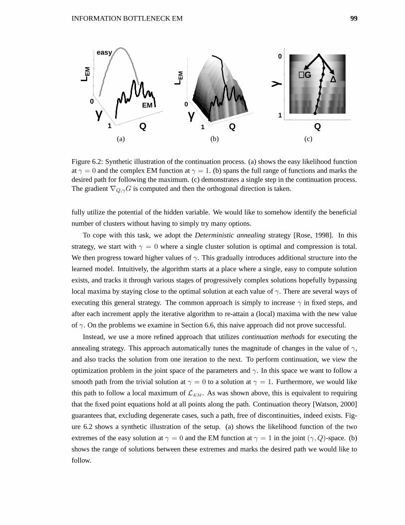
INFORMATION BOTTLENECK EM 99
0
1
LE
M
γγγγQ
easy
EM
LE
M
γγγγQ
0
1
∇∇∇∇G
γγ γγ
Q
0
1
∆∆∆∆
(a) (b) (c)
Figure 6.2: Synthetic illustration of the continuation process. (a) shows the easy likelihood functionat γ = 0 and the complex EM function at γ = 1. (b) spans the full range of functions and marks thedesired path for following the maximum. (c) demonstrates a single step in the continuation process.The gradient ∇Q,γG is computed and then the orthogonal direction is taken.
fully utilize the potential of the hidden variable. We would like to somehow identify the beneficial
number of clusters without having to simply try many options.
To cope with this task, we adopt the Deterministic annealing strategy [Rose, 1998]. In this
strategy, we start with γ = 0 where a single cluster solution is optimal and compression is total.
We then progress toward higher values of γ. This gradually introduces additional structure into the
learned model. Intuitively, the algorithm starts at a place where a single, easy to compute solution
exists, and tracks it through various stages of progressively complex solutions hopefully bypassing
local maxima by staying close to the optimal solution at each value of γ. There are several ways of
executing this general strategy. The common approach is simply to increase γ in fixed steps, and
after each increment apply the iterative algorithm to re-attain a (local) maxima with the new value
of γ. On the problems we examine in Section 6.6, this naive approach did not prove successful.
Instead, we use a more refined approach that utilizes continuation methods for executing the
annealing strategy. This approach automatically tunes the magnitude of changes in the value of γ,
and also tracks the solution from one iteration to the next. To perform continuation, we view the
optimization problem in the joint space of the parameters and γ. In this space we want to follow a
smooth path from the trivial solution at γ = 0 to a solution at γ = 1. Furthermore, we would like
this path to follow a local maximum of LEM . As was shown above, this is equivalent to requiring
that the fixed point equations hold at all points along the path. Continuation theory [Watson, 2000]
guarantees that, excluding degenerate cases, such a path, free of discontinuities, indeed exists. Fig-
ure 6.2 shows a synthetic illustration of the setup. (a) shows the likelihood function of the two
extremes of the easy solution at γ = 0 and the EM function at γ = 1 in the joint (γ,Q)-space. (b)
shows the range of solutions between these extremes and marks the desired path we would like to
follow.

100 INFORMATION BOTTLENECK EM
We start by characterizing such paths. Note that once we fix the parameters Q(T | Y ), the
M-step maximization of the parameters in P is fully determined as a function of Q. Thus, we take
Q(T | Y ) and γ as the only free parameters in our problem. As we have shown in Proposition 6.2.4,
when the gradient of the Lagrangian is zero, Eq. (6.4) holds for each value of t and y. Thus, we want
to consider paths where all of these equations hold. Rearranging terms and taking a log of Eq. (6.4)
we define
Gt,y(Q, γ) = − log Q(t | y) + (1− γ) log Q(t) + γ log P (x[y], y)− log Z(y, γ) (6.5)
Clearly, Gt,y(Q, γ) = 0 exactly when Eq. (6.4) holds for all t and y. Our goal is then to follow an
equi-potential path where all Gt,y(Q, γ) functions are zero starting from some small value of γ up
to the desired EM solution at γ = 1.
Suppose we are at a point (Q0, γ0), where Gt,y(Q0, γ0) = 0 for all t and y. We want to move
in a direction ∆ = (dQ, dγ) so that (Q0 + dQ, γ0 + dγ) also satisfies the fixed point equations. To
do so, we want to find a direction ∆, so that
∀t, y, ∇Q,γGt,y(Q0, γ0) ·∆ = 0 (6.6)
where ∇Q,γGt,y(Q0, γ0) is the gradient of Gt,y(Q0, γ0) with respect to the parameters Q and γ.
Computing these derivatives with respect to each of the parameters results in a derivative matrix
Ht,y(Q, γ) =(
∂Gt,y(Q,γ))∂Q(t|y)
∂Gt,y(Q,γ)∂γ
)(6.7)
Rows of the matrix correspond to each of the L = |T | × |Y | functions of Eq. (6.5), corresponding
to joint combinations of the |T | states of the bottleneck variable T and the |Y | = M number of
possible values of the instance identity variable Y . The columns correspond to the L parameters of
Q as well as γ. The entries correspond to the partial derivative of the function associated with the
row with respect to the parameter associated with the column.
To find a direction ∆ that satisfies Eq. (6.6) we need to satisfy the matrix equation
Ht,y(Q0, γ0)∆ = 0 (6.8)
In other words, we are trying to find a vector in the null-space of Ht,y(Q0, γ0)(Q0, γ0). The matrix
H is an L× (L+1) matrix and its null-space is defined by the intersection of L tangent planes, and
is of dimension L + 1 − Rank(Ht,y(Q, γ)). Numerically, excluding measure zero cases [Watson,
2000], we expect Rank(Ht,y(Q0, γ0)) to be full, i.e., L. Thus, a unique line that (up to scaling)
defines the null space, and we can choose any vector along it. To follow the path to our target
objective at γ = 1 we choose the direction that always increases γ (we discuss the choice of the

INFORMATION BOTTLENECK EM 101
length of this vector below). Returning to Figure 6.2, (c) illustrates this process. Shown is joint
(γ,Q)-space with the grey-level denoting the value of the likelihood function. At each point in the
learning process the gradient of G is evaluated and the orthogonal direction is taken to follow the
desired path.
Finding this direction, however, can be costly. Notice that Ht,y(Q, γ) is of size L(L + 1). This
number is quadratic in the training set size, and full computation of the matrix is impractical even
for small datasets. Instead, we resort to approximating Ht,y(Q, γ) by a matrix that contains only
the diagonal entries ∂Gt,y(Q,γ)∂Q(t|y) and the last column ∂Gt,y(Q,γ)
∂γ . While we cannot bound the extent of
this diagonal approximation, we note that the diagonal terms are also the most significant ones and
many off diagonal terms are zero. Once we make the approximation, we can solve Eq. (6.8) in time
linear in L. (See Appendix 6.5.3 for a full development of H and the computation of the orthogonal
direction. )
Note that once we find a vector ∆ that satisfies Eq. (6.8), we still need to decide on its length,
or the size of the step we want to take in that direction. There are various standard approaches, such
as normalizing the direction vector to a predetermined size. However, in our problem, we have a
natural measure of progress that stems from the tradeoff defined by the target Lagrangian LEM ,
where II(T ;Y ) increases when T captures more and more information about the samples during the
annealing procedure. That is, the “interesting” steps in the learning process occur when II(T ;Y )
grows. These are exactly the points where the balance between the two terms in the Lagrangian
changes and the second term grows sufficiently to allow the first term to increase II(T ;Y ). Using
II(T ;Y ) to gauge the progress of the annealing procedure is appealing since it is a non-parametric
measure that does not involve the form of the particular distribution of interest P . In addition, in
all runs II(T ;Y ) starts at 0, and is upper-bounded by the log of the cardinality of T and we are thus
given a scale of progress.
With this intuition at hand, we want to normalize the step size by the expected change in
II(T ;Y ). That is, we calibrate our progress with respect to the actual amount of regularization
applied at the current value of γ. At regions where II(T ;Y ) is not sensitive to changes in the pa-
rameters, we can proceed rapidly. On the other hand, if small changes in the parameters result in
significant changes of II(T ;Y ), then we want to carefully track the solution. Figure 6.3 illustrates
the difference between using a predetermined step of γ and partitioning II(T ;Y ) in order to deter-
mine the step size. It is evident the using II(T ;Y ) causes the method to concentrate on the region of
interest in terms of rapid change of the Lagrangian.
Formally, we compute ∇Q,γII(T ;Y ) and rescale the direction vector so that
(∇Q,γIIQ(T ;Y ))′ ·∆ = ε (6.9)
where ε is a predetermined step size that is a fraction of log |T |. We also bound the minimal and

102 INFORMATION BOTTLENECK EM
γγγγ0 0.2 0.4 0.6 0.8 1
0.5
1
1.5I(
T;Y
)
γγγγ0 0.2 0.4 0.6 0.8 1
0.5
1
1.5
I(T
;Y)
(a) (b)
Figure 6.3: Illustration of the step size calibration process. Both graphs show the change in infor-mation between T and Y as a function of γ. The circles denote values of γ to be evaluated. (a)shows naive calibration when fixed steps are taken in the γ range. (b) shows calibration that usesfixed steps in the information range. The grey circle shows the region of dramatic change of theLagrangian.
maximal change in γ so that we do not get trapped in too many steps or alternatively overlook the
regions of change.
Finally, although the continuation method takes us in the correct direction, the approximation as
well as inherent numerical instability can lead us to a suboptimal path. To cope with this situation,
we adopt a commonly used heuristic used in Deterministic annealing. At each value of γ, we slightly
perturb the current solution and re-iterate the self-consistent equations to converge on a solution. If
the perturbation leads to a better value of the Lagrangian, we take it as our current solution.
To summarize, our procedure works as follows: we start with γ = 0 for which only trivial
solutions exists. At each stage we compute the joint direction of γ and Q(T | Y ) that will leave the
fixed point equations intact. We then take a small step in this direction and apply IB-EM iterations
to attain the fixed point equilibrium at the new value of γ. We repeat these iterations until we reach
γ = 1.
6.4 Multiple Hidden Variables
The framework we described in the previous sections can easily accommodate learning networks
with multiple hidden variables simply by treating T as a vector of hidden variables. In this case, the
distribution Q(T | Y ) describes the joint distribution of the hidden variables for each value of Y ,
and P (T,X) describes their joint distribution with the attributes X in the desired network. Unfor-
tunately, if the number of variables T is large, the representation of Q(T | Y ) grows exponentially,
and this approach becomes infeasible.
One strategy to alleviate this problem is to force Q(T | Y ) to have a factorized form. This

INFORMATION BOTTLENECK EM 103
Gin = Q
X1 XnX1 XnY
T0 Tk
Gout = P
X1 Xn Y
T0
T1 Tk
Figure 6.4: Definition of networks for the Multivariate Information Bottleneck framework withmultiple hidden variables. Shown are Gin with the mean field assumption, and a possible choice forGout .
reduces the cost of representing Q and also the cost of performing inference. As an example, we
can require that Q(T | Y ) is factored as a product∏
i Q(Ti | Y ). This assumption is similar to the
mean field variational approximation (e.g., Jordan et al. [1998]).
In the Multivariate Information Bottleneck framework, different factorizations of Q(T | Y ) cor-
respond to different choices of networks Gin . For example, the mean field factorization is achieved
when Gin is such that the only parent of each Ti is Y , as in Figure 6.4. In general, we can consider
other choices where we introduce edges between the different Ti’s. For any such choice of Gin , we
get exactly the same Lagrangian as in the case of a single hidden variable. The main difference is
that since Q has a factorized form, we can decompose IIQ(T;Y ). For example, if we use the mean
field factorization, we get
IIQ(T;Y ) =∑
i
IIQ(Ti;Y )
Similarly, we can decompose IEQ[log P (X,T)] into a sum of terms, one for each family in P .
These two factorization can lead to tractable computation of the first two terms of the Lagrangian
as written in Proposition 6.2.1. Unfortunately, the last term IEQ[log Q(T)] cannot be evaluated
efficiently. Thus, we approximate this term as∑
i IEQ[log Q(Ti)]. For the mean field factorization,
the resulting Lagrangian (with this lower bound approximation) has the form
L+
EM =∑
i
IIQ(Ti;Y )− γ
(IEQ[log P (X, T )]−
∑
i
IEQ[log Q(Ti)]
)(6.10)
The form of L+
EM is valid, if Proposition 6.2.1 still holds for the case of multiple hidden vari-
ables. This is immediate if we make the following requirements, similar to those made for the case
of a single hidden variable:
1. Y is the instance identity;

104 INFORMATION BOTTLENECK EM
2. Gin is a Bayesian network structure such that all of the variables T are independent of X
given Y ; and
3. Gout is a Bayesian network structure such that Y is a child of T and has no other parents.
This implies that in Gout , Y is independent of all X given T.
The last requirement is needed so that we can set P (Y | T ) = Q(Y | T ) in the proof of Proposi-
tion 6.2.1. As in the case of a single hidden variable, we can now characterize fixed point equations
that hold in stationary points of the Lagrangian.
Proposition 6.4.1: Let L+
EM be defined via Gin and Gout as in Eq. (6.10). Assuming a mean field
approximation for Q(T | Y ), a (local) maximum of L+
EM is achieved by iteratively solving the
following self-consistent equations for every hidden variable i independently.
Q(ti | y) =1
Z(i, y, γ)Q(ti)
1−γ exp {γEP (ti, y)}
where
EP (ti, y) ≡ IEQ(T|ti,y)[log P (x[y],T)]
where Z(i, y, γ) is a normalizing constant and equals to
Z(i, y, γ) =∑
t′i
Q(t′i)1−γ exp
{γEP
(t′i, y
)}
See Appendix 6.5.2 for the proof.
The only difference from the case of a single hidden variables is in the form of the expectation
EP (ti, y). It is easy to see that when a single hidden variable is considered, and EP (ti, y) ≡
log P (x[y], t), the two forms coincide. It is also easy to see that this term decomposes into a sum of
expectations, one for each factor in the factorization of P . We note that only terms that average over
factors that involve Ti are of interest in EP (ti, y). All other terms do not depend on the value of Ti,
and can be absorbed by the normalizing constant. Thus, EP (ti, y) can still be computed efficiently.
A more interesting consequence (see theorem below) of this discussion is that when γ = 1,
maximizing L+
EM is equivalent to performing mean field EM [Jordan et al., 1998]. Thus, by using
the modified Lagrangian we generalize this variational learning principle, and as we show below
manage to reach better solutions.
The formulation is easily extensible to a general variational approximation of Q where G in
allows, in addition to the dependence of each Ti on Y , dependencies between the different Ti’s. In
this case, we get
IIQ(T;Y ) =∑
i
IIQ(Ti;PaGin
i)

INFORMATION BOTTLENECK EM 105
Similarly, IEQ[log P (X, T )] decomposes according to the joint families of Ti in P and in Q. That
is, each term in the decomposition depends on Ti, its parents PaGin
i in Gin , and its parents PaGout
i in
Gout . As in the case of the mean field variational approximation, the last term IEQ[log Q(T)] cannot
be evaluated efficiently. We approximate it using a decomposition that follows the structure of G in
as
IEQ[log Q(T)] ≈∑
i
IEQ
[log Q(Ti | T ∩Pa
Gin
i )]
(6.11)
We can now reformulate the results of Theorem 6.2.3 for this general case
Theorem 6.4.2: Let Q(T | Y ) decompose according to any structure Gin where all Ti’s are
descendents of Y and replace IEQ[log Q(T)] by a decomposition as defined in Eq. (6.11). Then for
the resulting Lagrangian
L+
EM = (1− γ)∑
i
IIQ(Ti;PaGin
i )− γF+ [Q,P ]
whereF+ [Q,P ] is defined as in Eq. (6.3), except that the above decomposition for both IEQ[log P (X, T )]
and IHQ(T | Y ) is used.
Proof: This is a direct result of the fact that in the proof of Theorem 6.2.3, no assumptions were
made of the form of Q.
The above theorem extends the formal relation of the Information Bottleneck target Lagrangian
and the EM functional for any form of variational approximation encoded by Gin . In particular,
when γ = 1, finding a local minimum of L+
EM is equivalent to finding a local maximum of the
likelihood function when the same variational approximation is used in the EM algorithm. Similarly,
we can derive the fixed point equations with each for different choices of Gin . The change to
Proposition 6.4.1 is simply a different decomposition for EP (i, y)
To summarize, the IB-EM algorithm of Section 6.2.2 can be easily generalized to handle multi-
ple hidden variables by simply altering the form of EP (ti, y) in the fixed point equations. All other
details, such as the continuation method, remain unchanged.
6.5 Proofs and Technical Computations
6.5.1 Fixed point equations:Single Hidden Variable
Proposition 6.2.4: Let LEM be defined via Gin and Gout as in Proposition 1. Q(T | Y ) is a
stationary point of LEM with respect to a fixed choice of P if and only if for all values t and y of T
and Y , respectively,
Q(t | y) =1
Z(y, γ)Q(t)1−γP (x[y], t])γ

106 INFORMATION BOTTLENECK EM
where and Z(y, γ) is a normalizing constant and equals to
Z(y, γ) =∑
t′
Q(t′)1−γP (x[y], t′])γ (6.12)
To prove the proposition we use the following
Lemma 6.5.1: [El-Hay and Friedman, 2001] Let Q(X) be a joint distribution over a set of random
variables X, that decomposes according to Q(X) =∏
i Q(Xi | Ui). Then
∂IEQ[f(X)]
∂Q(xi | ui)= Q(ui)IEQ(·|xi,ui)[f(X)] + IEQ
[∂f(x)
∂Q(xi,ui)
]
The following is an immediate results of that fact that Q(t) =∑
y′ Q(y′)Q(t|y′)
∂Q(T )
∂Q(t0 | y0)= Q(y0)1 {T = t0} (6.13)
We use this and an instantiation of the above lemma to prove the following:
Lemma 6.5.2:∂IIQ(T ;Y )
∂Q(t0 | y0)= Q(y0) log
Q(t0|y0)
Q(t0)
Proof: We define f(T, Y ) ≡ log Q(T,Y )Q(T )Q(Y ) = log Q(T |Y )
Q(T ) so that using Eq. (6.13), we can write
∂f(T, Y )
∂Q(t0 | y0)=
∂ log Q(T | Y )
∂Q(t0 | y0)−
∂ log Q(T )
∂Q(t0 | y0)
=1
Q(t0 | y0)1 {T = t0, Y = y0} −
Q(y0)
Q(t0)1 {T = t0}
Plugging this into Lemma 6.5.1, we get
∂IIQ(T ;Y )
∂Q(t0 | y0)= Q(y0)IEQ(·|t0,y0)
[log
Q(T | Y )
Q(T )
]+ IEQ
∂ log Q(T |Y )
Q(T )
∂Q(t0, y0)
= Q(y0) logQ(t0 | y0)
Q(t0)+ Q(y0)
Q(t0 | y0)
Q(t0 | y0)−∑
y
Q(y)Q(t0 | y)Q(y0)
Q(t0)
= Q(y0) logQ(t0 | y0)
Q(t0)+ Q(y0)
[1−
1
Q(t0)
∑
y
Q(y)Q(t0 | y)
]
= Q(y0) logQ(t0 | y0)
Q(t0)+ Q(y0) [1− 1]
= Q(y0) logQ(t0 | y0)
Q(t0)

INFORMATION BOTTLENECK EM 107
Using Eq. (6.13) and Lemma 6.5.1 with f(T, Y ) ≡ log Q(T ), the following is immediate
Lemma 6.5.3:
∂IEQ[log Q(T )]
∂Q(t0 | y0)= Q(y0) log Q(t0) + Q(t0)
1
Q(t0)Q(y0) = Q(y0) [log Q(t0) + 1]
Proof of the proposition: We want to find Q(T | Y ) that are stationary points of the Lagrangian
LEM and where the constraints∑
t Q(t | y) = 1 hold for any y. Thus, using Lagrange multipliers,
we want to optimize
L = IIQ(T ;Y )− γ (IEQ[log P (X, T )]− IEQ[log Q(T )]) +∑
y
λy
(∑
t′
Q(t′ | y)− 1
)
Since P is fixed, using Lemma 6.5.1 with f(Y,X, T ) ≡ log P (X, T ), we can write
∂IEQ[log P (X, T )]
∂Q(t0 | y0)= Q(y0) log P (x[y0], t0)
Combining this with Lemma 6.5.2 and Lemma 6.5.3, we get
∂LEM
∂Q(t0 | y0)= Q(y0) [log Q(t0 | y0)− (1− γ) log Q(t0) + γ − γ log P (x[y0], t0)] + λy0
Dividing by Q(y0) and equating to 0, we get after rearranging of terms
Q(t0|y0) = eλy0/Q(y0)+γQ(t0)1−γP (x[y0], t0)
γ (6.14)
This must hold for any value t0 and y0. Using∑
t Q(t | y0) = 1 we get
eλy0/Q(y0)+γ =1∑
t Q(t)1−γP (x[y0], t)γ
We get the desired result by plugging this into Eq. (6.14).
6.5.2 Fixed point equations:Multiple Hidden Variable
Proposition 6.4.1: Let L+
EM be defined via Gin and Gout as in Eq. (6.10). Assuming a mean field
approximation for Q(T | Y ), a (local) maximum of L+
EM is achieved by iteratively solving the
following self-consistent equations for every hidden variable i independently.
Q(ti | y) =1
Z(i, y, γ)Q(ti)
1−γ expγEP(ti,y)

108 INFORMATION BOTTLENECK EM
where
EP (ti, y) ≡ IEQ(T|ti,y)[log P (x[y],T)]
where Z(i, y, γ) is a normalizing constant and equals to
Z(i, y, γ) =∑
t′i
Q(t′i)1−γ expγEP(t′i,y)
Proof: Using the mean field assumption, the information and entropy terms in the Lagrangian
decompose as follows
L+
EM =∑
i
IIQ(Ti;Y )− γ
(IEQ[log P (X, T )]−
∑
i
IEQ[log Q(Ti)]
)
When computing the derivative with respect to the parameters of a specific variables Ti, the only
change from the case of single hidden variable, is in the derivative of IEQ[log P (X, T )] given fixed
P . Again using Lemma 6.5.1 with f(Y,X, T ) ≡ log P (X, T ) we get
∂IEQ[log P (X,T)]
∂Q(ti0 | y0)= IEQ(T |ti0,y0)[log P (x[y0],T)]
from which we get the change from Proposition 6.2.4 to Proposition 6.4.1 for the case of multiple
hidden variables.
6.5.3 Computing the Continuation Direction
We now develop the formulas needed to perform continuation as described in Section 6.3 for the
case of a single hidden variable T . Consider again Eq. (6.5), where we now write the normalization
term Z(y, γ) explicitly:
Gt,y(Q, γ) = − log Q(t | y) + (1− γ) log Q(t) + γ log P (x[y], t)
− log∑
t′
exp(1−γ) log Q(t′)+γ log P (x[y],t′)
︸ ︷︷ ︸Z(y,γ)
(6.15)
We want to compute the derivative of Gt,y(Q, γ) with respect to the parameters and γ, and and then
use the orthogonal direction for continuation. The will follow a direction in which the fix point
equations remain unchanged, and the local maximum is tracked. To do so, we start by expressing
log P (x[y], t) as a function of the parameters Q.

INFORMATION BOTTLENECK EM 109
The maximum likelihood parameters of log P (X, T ) for the conditional distribution of the chil-
dren Xi of T in Gout are
θxi|pai,t=
∑y Q(y)Q(t|y)1 {xi[y] = xi,pai[y] = pai}+ α(xi,pai, t)∑
y Q(y)Q(t|y)1 {pai[y] = pai}+ α(pai, t)≡N (xi,pai, t)
N (pai, t)(6.16)
where 1 {} is the indicator function, α() are the hyper-parameters of the Dirichlet prior distribution
(see Section 2.2.2) and N are used to denote the total counts (including prior) used for estimation.
Similarly the maximum likelihood parameters of the distribution of T given its parents are
θt|pat=
∑y Q(y)Q(t|y)1 {pat[y] = pat}+ α(pat, t)∑
y Q(y)1 {pat[y] = pat}+ α(pat)≡N (pat, t)
N (pat)(6.17)
We now consider each term in Gt,y(Q, γ) and compute its derivative with respect to these parameters
of Q.
Computation of ∂ log P (x[y],t)∂Q(t0|y0)
The derivatives of the parameters expressed in Eq. (6.16) are:
∂θxi|pai,t
∂Q(t0|y0)
= Q(y0)N (pai,t)
2
[1 {xi[y0] = xi,pai[y0] = pai}N (pai, t)− 1 {pai[y0] = pai}N (xi,pai, t)
]
= Q(y0)1{pai[y0]=pai}N (pai,t)
2
(1 {xi[y0] = xi}N (pai, t)−N (xi,pai, t)
)
(6.18)
for t = t0 and is zero otherwise. Similarly, the derivatives of the parameters of Eq. (6.17) is
∂θt|pat
∂Q(t0 | y0)=
Q(y0)
N (pat)2
[1 {pat[y0] = pat}N (pat)− 0] =Q(y0)
N (pat)1 {pat[y0] = pat} (6.19)
for t = t0, and is zero otherwise. The log-probability of a specific instance can be written as
log P (x[y], t) = log θt|pat[y] +
∑
i∈Cht
log θxi|pai,t[y] +
∑
i6=t,Cht
log θxi|pai[y] (6.20)
where Cht denotes the children of T in Gout and θt|pat[y] is the parameter corresponding to the
values appearing in instance y. We note that the last summation does not depend on the parameters

110 INFORMATION BOTTLENECK EM
Q(t | y), and by plugging Eq. (6.18) and Eq. (6.19) into Eq. (6.20), we get
∂ log P (x[y], t)
∂Q(t0 | y0)=
1
θt|pat[y]
∂θt|pat[y]
∂Q(t0 | y0)+∑
i∈Cht
1
θxi|pai,t[y]
∂θxi|pai,t[y]
∂Q(t0 | y0)
= Q(y0)
[1{pat[y0]=pat[y]}N (pat)θt|pat
[y0]
+∑
i∈Cht
1{pai[y0]=pai[y]}N (pai,t)
2θxi|pai[y0]
(1 {xi[y] = xi[y0]}N (pai, t)−N (xi,pai, t)
)]
≡ Q(y0)D(y, t)(6.21)
where in the last line we use D(y, t) to denote the expression in the square brackets.
Computation of ∂ log Z(y0,γ)∂Q(t0|y0)
Using Eq. (6.13) from Section 6.5.1 and the above, we can write
∂ (1− γ) log Q(t) + γ log P (x[y], t)
∂Q(t0 | y0)= Q(y0)
[1− γ
Q(t)+ γD(y, t)
](6.22)
We can now use Eq. (6.22) to write the derivative of Z(y, γ) since it is a summation over similar
expressions
∂ log Z(y0,γ)∂Q(t0|y0)
= 1Z(y0,γ) exp(1−γ) log Q(t0)+γ log P (x[y],t0) Q(y0)
[1−γQ(t0) + γD(y0, t0)
]
= 1Z(y0,γ)Q(y0)Q(t0)
1−γP (x[y], t0)γ[
1−γQ(t0) + γD(y0, t0)
]
= Q(y0)Q(t0 | y0)[
1−γQ(t0) + γD(y0, t0)
] (6.23)
where the last equality follows from Proposition 6.2.4.
Computation of ∂Gt,y(Q,γ)∂Q(t0|y0)
We combine Eq. (6.22) and Eq. (6.23) to write
∂Gt,y(Q, γ)
∂Q(t0 | y0)= −1 {y = y0}+ Q(y0) [1−Q(t0 | y0)]
[1− γ
Q(t0)+ γD(y0, t0)
](6.24)
Computation of ∂ log Z(y,γ)∂γ
The only term that is not immediate is the derivative of Z(y, γ) with respect to γ
∂ log Z(y, γ)
∂γ=
1
Z(y, γ)
∑
t′
exp(1−γ) log Q(t′)+γ log P (x[y],t′)[− log Q(t′) + log P (x[y], t′)
]
=∑
t′
1
Z(y, γ)Q(t′)1−γP (x[y], t′)γ
[− log Q(t′) + log P (x[y], t′)
]

INFORMATION BOTTLENECK EM 111
=∑
t′
Q(t′|y)[log P (x[y], t′)− log Q(t′)
]
from which follows
∂Gt,y(Q, γ)
∂γ= log P (x[y], t)− log Q(t)−
∑
t′
Q(t′|y)[log P (x[y], t′)− log Q(t′)
](6.25)
Computation of the continuation direction
We can now compute all the elements of the derivative matrix of Eq. (6.7)
Ht,y(Q, γ) =(
∂Gt,y(Q,γ))∂Q(t|y)
∂Gt,y(Q,γ)∂γ
)
To compute the orthogonal direction to the derivative, we solve Eq. (6.8)
H(Q, γ)∆ = 0
As noted in Section 6.3, this can be prohibitively expensive and we resort to H(Q, γ) with a diagonal
approximation for elements of ∂Gt,y(Q,γ)∂Q(t|y) computed in Eq. (6.24). We denote by hy,t the diagonal
entry for Y = y and T = t and hγy,t the corresponding derivative with respect to γ. We then have to
solve a set of equations of the form
dt,yhy,t + dγhγy,t = 0
where dt,y and dγ are the elements of ∆. Setting dγ = 1 (an equivalent solution up to scaling) we
get the unique solution
dt,y = −hγ
y,t
hy,t
Normalizing ∆ using the derivative of IIQ(T ;Y ) as described in Eq. (6.9) can now be easily com-
puted given the Lemma 6.5.2 in Section 6.5.1.
Multiple Hidden Variables
When computing the derivative with respect to the parameters associated with a specific hidden vari-
able ti, the only change in Gt,y(Q, γ) is that log P (x[y], t) is replaced by the term IEQ(T|ti,y)[log P (x[y],T)].
In this case we simply compute the expectation of Eq. (6.21) over the T ’s that are in the Markov
blanket of ti. The rest of the details remain the same.

112 INFORMATION BOTTLENECK EM
0 20 40 60 80 100
-435.5
-434.5
-433.5
Percentage of random runs
Tes
t L
L /
inst
ance
mean field EM~2.6 hours
single IB-EM ~85 hours
each exact EM> 17 hours
(a) (b)
Figure 6.5: (a) A quadrant based hierarchy structure with 21 hidden variables for modeling 16× 16images in the Digit domain. (b) Test log-loss of the IB-EM algorithm for the model of (a) comparedto the cumulative performance of 50 random EM and mean field EM runs.
6.6 Experimental Validation: Parameter Learning
To evaluate the IB-EM method for the task of parameter learning, we examine its generalization
performance on several types of models on three real-life datasets. In each architecture, we consider
networks with hidden variables of different cardinality, where for now we use the same cardinality
for all hidden variables in the same network. We now briefly describe the datasets and the model
architectures we use.
• The Stock dataset records up/same/down daily changes of 20 major US technology stocks
over a period of several years [Boyen et al., 1999]. The training set includes 1213 samples
and the test set includes 303 instances. We trained a Naive Bayes hidden variable model
where the hidden variable is a parent of all the observations.
• The Digits dataset contains 7291 training instances and 2007 test instances from the USPS
(US Postal Service) dataset of handwritten digits (see http://www.kernel-machines.org/data.html).
An image is represented by 256 variables, each denoting the gray level of one pixel in a 16×16
matrix. We discretized pixel values into 10 equal bins.
On this dataset we tried several network architectures. The first is a Naive Bayes model with a
single hidden variable. In addition, we examined more complex hierarchical models. In these
models we introduce a hidden parent to each quadrant of the image recursively. The 3-level
hierarchy has a hidden parent to each 8x8 quadrant, and then another hidden variable that is
the parent of these four hidden variables. The 4-level hierarchy starts with 4x4 pixel blocks
each with a hidden parent. Every 4 of these are joined into an 8x8 quadrant by another level
of hidden variables, totaling 21 hidden variables, as illustrated in Figure 6.5(a).

INFORMATION BOTTLENECK EM 113
• The Yeast dataset contains measurements of the expression of the Baker’s yeast genes in 173
experiments [Gasch et al., 2000]. These experiments measure the yeast response to changes
in its environmental conditions. For each experiment the expression of 6152 genes were
measured. We discretized the expression levels of genes into ranges down/same/up by using a
threshold of one standard deviation from above and below the gene’s mean expression across
all experiments. In this dataset, we treat each gene as an instance that is described by its
behavior in the different experiments. We randomly partitioned the data into 4922 training
instances (genes) and 1230 test instances.
The model we use for this dataset has an hierarchical structure with 19 hidden variables in
a 4-level hierarchy that was determined by the biological expert based on the nature of the
different experiments, as illustrated schematically in Figure 6.6. In this structure, 5–24 simi-
lar conditions (filled nodes) such as different hypo-osmotic shocks are children of a common
hidden parent (unfilled nodes). These hidden parents are in their turn children of further ab-
straction of conditions. For example, the heat shock and heat shock with oxidative stress
hidden nodes, are both children of a common more abstract heat node. A root hidden vari-
able is the common parents of these high-level abstractions. Intuitively, each hidden variable
encodes how the specific instance (a gene) is altered in the relevant groups of conditions.
As a first sanity check, for each model (and each cardinality of hidden variables) we performed
50 runs of EM with random starting points. The parameter sets learned in these different runs have
a wide range of likelihoods both on the training set and the test set. These results (on which we
elaborate below), indicate that these learning problems are challenging in the sense that EM runs
can be trapped in markedly different local maxima.
Next, we considered the application of IB-EM on these problems. We performed a single IB-EM
run on each problem and compared it to the 50 random EM runs, and also to 50 random mean field
EM runs. For example, Figure 6.5 compares the test set performance (log-likelihood per instance)
of these runs on the Digit dataset with a 4-level hierarchy of 21 hidden variables with 2 states each.
The solid line shows the performance of the IB-EM solution at γ = 1. The two dotted lines show
the cumulative performance of the random runs. As we can see, the IB-EM model is superior to
all the mean field EM runs, as well as all of the exact EM runs. Figure 6.6 shows the result for the
biological expert constructed hierarchy of Yeast dataset with binary variables. As can be seen, in
this harder domain, the superiority of the exact EM runs over mean field EM runs is more evident.
Yet, the IB-EM run which also use the mean field approximation, is still able to surpass all of the
50 random exact EM runs.
It is important to note the time required by these runs, all on a Pentium IV 2.4 GHz machine.
For the Digit dataset, a single mean field EM run requires approximately 2.5 hours, an exact EM
run requires roughly 17 hours, and the single IB-EM run requires just over 85 hours. As the IB-EM

114 INFORMATION BOTTLENECK EM
mean field EM~0.5 hours/run
single IB-EM ~6 hours
exact EM> 60 hours/run
-151.5
-150.5
-149.5
-148.5
-147.5
0 20 40 60 80 100
Percentage of random runs
Tes
t L
L /
inst
ance
(a) (b)
Figure 6.6: (a) A structure constructed by the biological expert for the Yeast dataset based on prop-erties of different experiments. 5-24 similar conditions (filled nodes) are aggregated by a commonhidden parent (unfilled nodes). These hidden nodes are themselves children of further abstractionnodes of similar experiments, which in their turn are children of the single root node. (b) Compar-ison of test performance when learning the parameters of the structure of (a) with binary variables.Shown is test log-likelihood per instance of the IB-EM algorithm and the cumulative performanceof 50 random EM as well as 50 random mean field EM runs.
run reaches a solution that is better than all of this runs, it offers an appealing performance to time
tradeoff. This is even more evident for the Yeast dataset where the structure is somewhat more
complex and the difference between exact learning and the mean field approximation is greater. For
this dataset, the single IB-EM is still superior and takes significantly less time than a single exact
EM.
Figure 6.7 compares the test log-likelihood per instance performance of our IB-EM algorithms
and 50 random EM runs for a range of models for the Stock, Digit and Yeast datasets. In most
cases, IB-EM is better than 80% of the EM runs and is often as good or better than the best of
them. The advantage of IB-EM is particularly pronounced for the more complex models with
higher cardinalities. Table 6.1 provides more details of these runs including train performance
and comparison to 50 random mean field EM runs.
We also compared the IB-EM method to the perturbation method of Elidan et al. [2002]. Briefly,
their method alters the landscape of the likelihood by perturbing the relative weight of the samples
and progressively diminishing this perturbation as a factor of the temperature parameter. In the
Stock dataset, the perturbation method initialized with a starting temperature of 4 and cooling factor
of 0.95, had performance similar to that of IB-EM. However, the running time of the perturbation
method was an order of magnitude longer. For the other datasets we considered above, running
the perturbation method with the same parameters proved to be impractical. When we used more
efficient parameter settings, the perturbation method’s performance was significantly inferior to

INF
OR
MA
TIO
NB
OT
TL
EN
EC
KE
M115
Train Log-Likelihood Test Log-LikelihoodModel IB-EM Random EM Mean Field EM IB-EM Random EM Mean Field EM
%< 100% 80% %< 100% 80% %< 100% 80% %< 100% 80%StockC=3 -19.91 62% -19.90 -19.90 -19.90 76% -19.88 -19.89C=4 -19.47 98% -19.46 -19.52 -19.52 96% -19.52 -19.62C=5 -19.16 94% -19.15 -19.24 -19.31 98% -19.30 -19.39DigitC=5 -429.95 36% -428.67 -429.11 -439.91 56% -439.03 -439.47C=10 -411.44 100% -411.72 -413.96 -425.33 100% -425.36 -427.05DigH3C=2 -442.02 100% -442.02 -442.29 100% -442.03 -442.20 -450.812 92% -450.76 -450.92 82% -450.76 -450.84C=3 -428.77 100% -428.85 -429.02 100% -428.83 -429.02 -437.798 98% -437.74 -438.20 98% -437.74 -438.04DigH4C=2 -425.43 100% -425.54 -425.81 100% -425.61 -425.94 -433.279 100% -433.30 -433.55 100% -433.40 -433.71C=3 -407.60 100% -407.75 -408.56 100% -408.49 -408.83 -415.798 100% -415.88 -416.48 100% -416.37 -416.77YeastC=2 -148.13 100% -148.32 -148.79 100% -148.89 -149.71 -147.48 100% -147.51 -147.87 100% -147.92 -148.78C=3 -139.44 100% -139.58 -140.05 100% -140.09 -140.87 -138.38 100% -138.57 -139.00 100% -139.06 -139.92C=4 -136.36 100% -136.72 -136.97 100% -137.72 -138.28 -135.65 100% -135.96 -136.16 100% -136.92 -137.34
Table 6.1: Comparison of the IB-EM algorithm, 50 runs of EM with random starting points, and 50 runs of mean field EM from the samerandom starting points. Shown are train and test log-likelihood per instance for the best and 80th percentile of the random runs. Also shown isthe percentile of the runs that are worse than the IB-EM results. Datasets shown include a Naive Bayes model for the Stock dataset and the Digitdataset; a 3 and 4 level hierarchical model for the Digit dataset (DigH3 and DigH4); and an hierarchical model for the Yeast dataset. For eachmodel we show several cardinalities for the hidden variables, shown in the first column.

116 INFORMATION BOTTLENECK EM
Tes
t log
-like
lihoo
d / i
nsta
nce
StockC=3 C=4 C=5 C=6 C=7 C=8 C=9 C=10
-20.4
-20
-19.6
-19.2
-18.8
Range of random EM runsRange of random EM runs20%-80% precentileIB-EM
Digit Digit HierC=5 C=10C=5 C=10 C=2 C=3C=2 C=3
-430
-420
-410
YeastC=2 C=3 C=4
-152
-148
-144
-140
-136
Figure 6.7: Comparison of log-likelihood per instance test performance of the IB-EM algorithm(black ’X’) and 50 runs of EM with random starting points. The vertical line shows the range ofthe random runs and boxes mark the 20%-80% range. Datasets shown (x-axis) include a NaiveBayes model for the Stock dataset and the Digit dataset; a 4 level hierarchical model for the Digitdataset (Digit Hier); a hierarchical model for the Yeast dataset. For each model we show severalcardinalities for the hidden variables, shown in the x-axis.
that of IB-EM. These results do not contradict those of Elidan et al. [2002] who showed some
improvement for the case of parameter learning but mainly focused on structure learning, with and
without hidden variables.
To demonstrate the effectiveness of the continuation method we examine IB-EM during the
progress of γ. Figure 6.8 illustrates the progression of the algorithm on the Stock dataset. (a)
shows training log-likelihood per instance of parameters in intermediate points in the process. This
panel also shows the values of γ evaluated during the continuation process (circles). These were
evaluated using the predicted change in II(T ;Y ) shown in (b). As we can see, the continuation
procedure focuses on the region where there are significant changes in II(T ;Y ) approximately cor-
responding the areas of significant changes in the likelihood. For both the Stock and Digit datasets,
we also tried changing γ naively from 0 to 1 as in standard annealing procedures, without per-
forming continuation. This procedure often “missed” the superior local maxima even when a large
number (1000) of γ values were used in the process. In fact, in most runs the results were no better
than the average random EM run emphasizing the importance of the continuation in the annealing
process.
6.7 Learning Structure
Up until now, we were only interested in parameter learning. However, in real life it is often not
the case that the structure is given. A structure that is too simple will not be able to faithfully cap-
ture the distribution, while an overly complex structure will deteriorate our ability to learn. In this

INFORMATION BOTTLENECK EM 117
γγγγ0 0.2 0.4 0.6 0.8 1
-23
-21
-19
Tra
in li
kelih
oo
d
IB-EM
Best of EM
0 0.2 0.4 0.6 0.8 1
0.5
1
1.5
I(T
;Y)
γγγγ(a) (b)
Figure 6.8: The continuation process for a Naive Bayes model on the Stock data set. (a) Showsthe progress of training likelihood as a function of γ compared to the best of 50 EM random runs.Black circles illustrate the progress of the continuation procedure by denoting the value of γ at theend of each continuation step. Calibration is done using information between the hidden variable Tand the instance identity Y shown in (b) as a function of γ.
section we consider the case where the set of hidden variables is fixed and their cardinalities are
known, and we want to learn the network structure. Clearly, this problem is harder than simple
parameter learning, which is just one of the tasks we have to perform in this scenario. The common
approach to this model selection task is to use a score-based approach where we search for a struc-
ture that maximizes some score. Common scores such as the BDe score [Heckerman et al., 1995a]
balance the likelihood achieved by the model and its complexity. Thus, model selection is achieved
independently of the search procedure used (see Section 2.3 for more details).
We now aim to extend the IB-EM framework for the task of structure learning using a score-
based approach. Naively, we could simply consider different structures and for each one apply the
IB-EM procedure to estimate parameters, and then evaluate its generalization ability using the score.
Such an approach is extremely inefficient, since it spends a non-trivial amount of time to evaluate
each potential candidate structure. In this work we advocate a strategy that is based on the Struc-
tural EM framework of Friedman [1997]. In Structural EM (see Section 2.4), we use the completion
distribution Q that is a result of the E-Step to compute expected sufficient statistics. That is, instead
of Eq. (2.7) we use Eq. (2.16), where in our case the completion distribution Q(H | O, θold) is
simply Q(T | Y ). These statistics are then used in the M-step when structure modification steps are
evaluated. Thus, instead of assuming that the target structure Gout is fixed, we define the Lagrangian
as a function of the pair (Gout , θ). Then, in the M-step, we can consider different choices of Gout
and evaluate how each of them changes the score. Given the expected statistics, the problem is
identical in form to learning from a fully observed dataset and computation of the score is similar.
This facilitates an efficient greedy search procedure that uses local edge modification to the network
structure. The EM procedure of Section 6.2.2 is thus revised as follows:

118 INFORMATION BOTTLENECK EM
• E-step : Maximize −LEM by varying Q(T | Y ) while holding P fixed.
• M-step: While holding Q fixed:
– Search for the structure Gout of P that maximizes ScoreBDe(G : D), using the sufficient
statistics of Q.
– Maximize −LEM by varying the parameters of P using the structure Gout selected.
In practice, since the BDe score is not a linear function of the sufficient statistics, we approx-
imate it in the M-step using the Cheeseman-Stutz [Cheeseman et al., 1988] approximation. It is
important to note the distinction between the optimization of the Lagrangian and that of the score.
Specifically, optimizing the Lagrangian involves maximization of the likelihood along with an infor-
mation theoretic regularization term that does not depend on P . On the other hand, optimization of
the structure is performed using the BDe model selection score. This is mathematically valid since
each optimization step is ignorant of the inner mechanics of the other step. However, one might
wonder why the use of a score is needed at all if regularization is already present in the form of the
information theoretic term in the Lagrangian. It is easy to understand the reason for this if we look at
the final stage of learning when γ = 1. At this point, as we have shown, optimizing the Lagrangian
is equivalent to optimizing the EM objective. Using the same objective to adapt structure will result
in dense structures. In particular, it will be beneficial to add an edge between any two variables
that are not perfectly independent in the training data. Thus, while the regularization encoded in the
Lagrangian is needed to smooth the parametric EM problem, a model selection regularization via a
score is also needed to constrain the network structure.
Using the Structural EM framework allows us to apply our framework to structure learning and
to use various search operators as simple plug-ins. For general Bayesian networks, for example, one
can consider the standard add, delete and reverse edge operators. The only requirement in this case
is that a hidden variable is constrained to be non-leaf, in which case it becomes redundant and can
be marginalized out. In addition, as in the case of learning parameters, we are still guaranteed to
converge for a given value of γ. However, as in parametric EM, convergence is typically to a local
maximum. In fact, the problem now has two facets: First, local maxima that result from evaluation
of Q in the E-step. Second, local maxima in the discrete structure search space due to the greedy
nature of the search algorithm.
Although the method described above applies for any Bayesian network structure, for concrete-
ness we focus on learning hierarchies of hidden variables in the following sections. In this sub-class
of networks each variable has at most one parent, and that parent has to be a hidden variable. This
implies that the hierarchy of hidden variables captures the dependencies between the observed at-
tributes. Since we are dealing with hierarchies we consider search steps that replace the parent of a

INFORMATION BOTTLENECK EM 119
0 0.2 0.4 0.6 0.8 1
1
2
3
4
5
6
7
8
γE
ffect
ive
Car
dina
lity
Figure 6.9: Effective cardinality as a function of γ during the learning process for the Stock datasetusing a Naive Bayes model. Cardinality is evaluated using local decomposition of the BDe score.
variable by one of the hidden variables. Such moves preserve the overall hierarchy structure, repo-
sitioning a single observed variable, or a sub-hierarchy. We apply these steps in a greedy manner,
from the one that leads to the largest improvement, as long as the resulting hierarchy is acyclic.
6.8 Learning Cardinality
In real life, it is often the case that we do not know the cardinality of a hidden variable. In a clustering
application, for example, we typically do not know of a beneficial number of clusters and need to
either use some arbitrary choice or spend time evaluating several possibilities. Naively, we might
try to set a high cardinality so that we can capture all potential clusters. However, this approach can
lead to bad generalization performance due to over-representation. The discussion in Section 6.3 on
the behavior of the model as a function of γ provides insight on the effect of cardinality selection.
When examining the models during the continuation process, we observe that for lower values of
γ the effective cardinality of the hidden variable is smaller than its cardinality in the model (we
elaborate on how this is measured below). Figure 6.9 shows an example of this phenomenon for the
Naive Bayes model of the Stock dataset. Thus, limiting the cardinality of the hidden variable is in
effect similar to stopping the continuation process at some γ < 1. This is, by definition, equivalent
to using a regularized version of the EM objective, which can avoid overfitting.
The most straightforward approach to learning the cardinality of a hidden variable is simply to
try a few values, and for each value apply IB-EM independently. We can then compare the value
of the EM objective (at γ = 1) corresponding to the different cardinalities. However, models with
higher cardinality will achieve a higher likelihood and will thus always be chosen as preferable by
the Lagrangian, at the risk of overfitting the training data. In the previous section we discussed
the use of a model selection score as a measure for preferring one network structure over another.

120 INFORMATION BOTTLENECK EM
The same score can also be readily applied for this scenario of cardinality selection. Whether the
complexity is a result of a dense structure or an increased number of parameters due to a high
cardinality of a variable, all common scores balance the likelihood with the model complexity,
either explicitly as in the case of the MDL score [Lam and Bacchus, 1994] or implicitly as in the
case of the Bayesian (BDe) score [Heckerman et al., 1995a]. Thus, similarly to structure learning,
we use the Lagrangian when estimating parameters and turn to the score when performing the black-
box model selection step. One problem with this simple approach is that it can be extremely time
consuming. If we want to try K different cardinalities for each hidden variable, we have to carry
out |H|K independent IB-EM runs, where |H| is the number of hidden variables.
The intuition that the “effective” cardinality of the hidden variable will increase as we consider
larger values of γ suggests that we increasing the model complexity during the continuation process.
A simple method is as follows. At each stage allow the model an extra, seemingly redundant, state
for the hidden variable. As soon as this state is utilized, we increase the cardinality by adding a
new “spare” state. The annealing process, by nature, automatically utilizes this new state when it
is beneficial to do so. The task we face is to determine when all the states of a hidden variables
are being utilized and therefore a new redundant state is needed. Intuitively, a state of a variable is
being used if it captures a distinct behavior that is not captured by other states. That is, for any state
i, no other state j is similar.
To determine whether state i is different than all other states, we start by evaluating the cost
that we incur due to the merging of state i with another state j. We denote by ij a new state that
combines both i and j and alter Q so that
Q(T = ij | Y = y) = Q(T = i | Y = y) + Q(T = j | Y = y) (6.26)
We then use this to reestimate the parameters of P in the M-step, and examine the resulting change
to the Lagrangian. As shown in Slonim et al. [2002], the difference in the Lagrangian before and
after the merge is a sum of Jensen-Shannon divergence terms that measure the difference between
the conditional distribution of each child variable given the two states of the hidden variable. This is
in fact the change in likelihood of the model resulting from merging the states and can be computed
efficiently.
Now that we have the change in the Lagrangian due to the merging of state i with state j, we
have to determine whether this change is significant. As already noted, using more states will always
improve the likelihood so that the difference in the Lagrangian is not sufficient for model selection.
Instead, we can use the BDe score to take into account both the improvement to the likelihood and
the change in the model complexity as in Elidan and Friedman [2001]. One appealing property of
the BDe score is that it is locally decomposable. That is, Eq. (2.15) decomposes according to the
different values of each variables. Thus, the difference between the BDe score after and before the
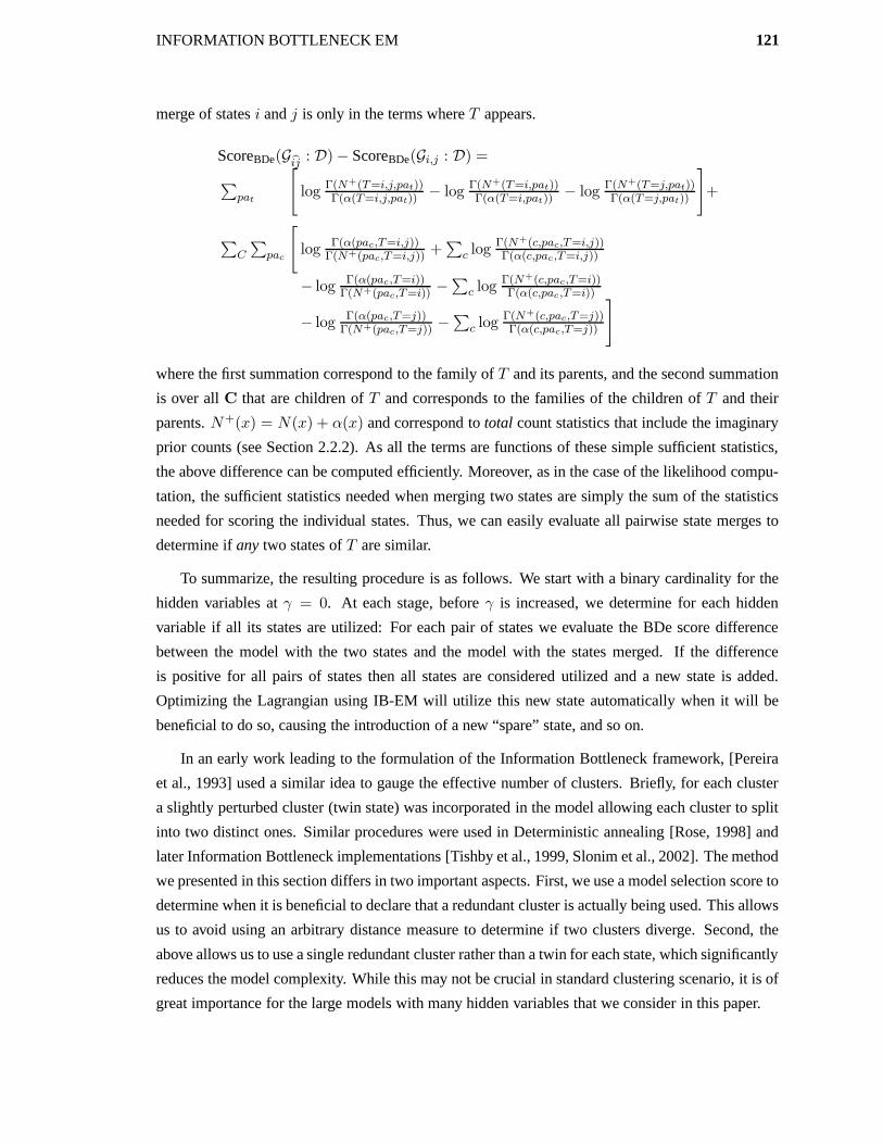
INFORMATION BOTTLENECK EM 121
merge of states i and j is only in the terms where T appears.
ScoreBDe(Gbij : D)− ScoreBDe(Gi,j : D) =
∑pat
[log Γ(N+(T=i,j,pat))
Γ(α(T=i,j,pat))− log Γ(N+(T=i,pat))
Γ(α(T=i,pat))− log Γ(N+(T=j,pat))
Γ(α(T=j,pat))
]+
∑C
∑pac
[log Γ(α(pac,T=i,j))
Γ(N+(pac,T=i,j)) +∑
c log Γ(N+(c,pac,T=i,j))Γ(α(c,pac,T=i,j))
− log Γ(α(pac,T=i))Γ(N+(pac,T=i)) −
∑c log Γ(N+(c,pac,T=i))
Γ(α(c,pac,T=i))
− log Γ(α(pac,T=j))Γ(N+(pac,T=j)) −
∑c log Γ(N+(c,pac,T=j))
Γ(α(c,pac,T=j))
]
where the first summation correspond to the family of T and its parents, and the second summation
is over all C that are children of T and corresponds to the families of the children of T and their
parents. N+(x) = N(x) + α(x) and correspond to total count statistics that include the imaginary
prior counts (see Section 2.2.2). As all the terms are functions of these simple sufficient statistics,
the above difference can be computed efficiently. Moreover, as in the case of the likelihood compu-
tation, the sufficient statistics needed when merging two states are simply the sum of the statistics
needed for scoring the individual states. Thus, we can easily evaluate all pairwise state merges to
determine if any two states of T are similar.
To summarize, the resulting procedure is as follows. We start with a binary cardinality for the
hidden variables at γ = 0. At each stage, before γ is increased, we determine for each hidden
variable if all its states are utilized: For each pair of states we evaluate the BDe score difference
between the model with the two states and the model with the states merged. If the difference
is positive for all pairs of states then all states are considered utilized and a new state is added.
Optimizing the Lagrangian using IB-EM will utilize this new state automatically when it will be
beneficial to do so, causing the introduction of a new “spare” state, and so on.
In an early work leading to the formulation of the Information Bottleneck framework, [Pereira
et al., 1993] used a similar idea to gauge the effective number of clusters. Briefly, for each cluster
a slightly perturbed cluster (twin state) was incorporated in the model allowing each cluster to split
into two distinct ones. Similar procedures were used in Deterministic annealing [Rose, 1998] and
later Information Bottleneck implementations [Tishby et al., 1999, Slonim et al., 2002]. The method
we presented in this section differs in two important aspects. First, we use a model selection score to
determine when it is beneficial to declare that a redundant cluster is actually being used. This allows
us to avoid using an arbitrary distance measure to determine if two clusters diverge. Second, the
above allows us to use a single redundant cluster rather than a twin for each state, which significantly
reduces the model complexity. While this may not be crucial in standard clustering scenario, it is of
great importance for the large models with many hidden variables that we consider in this paper.
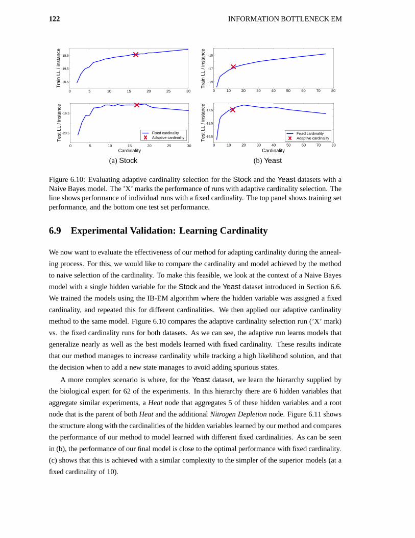
122 INFORMATION BOTTLENECK EM
-20.5
-19.5
0 5 10 15 20 25 30
-20.5
-19.5
-18.5T
rain
LL
/ ins
tanc
e
0 5 10 15 20 25 30Cardinality
Tes
t LL
/ ins
tanc
e
Adaptive cardinalityFixed cardinality
0 10 20 30 40 50 60 70 80
-19
-17
-15
0 10 20 30 40 50 60 70 80
-19.5
-18.5
-17.5
Cardinality
Adaptive cardinalityFixed cardinality
Tra
in L
L / i
nsta
nce
Tes
t LL
/ ins
tanc
e
(a) Stock (b) Yeast
Figure 6.10: Evaluating adaptive cardinality selection for the Stock and the Yeast datasets with aNaive Bayes model. The ’X’ marks the performance of runs with adaptive cardinality selection. Theline shows performance of individual runs with a fixed cardinality. The top panel shows training setperformance, and the bottom one test set performance.
6.9 Experimental Validation: Learning Cardinality
We now want to evaluate the effectiveness of our method for adapting cardinality during the anneal-
ing process. For this, we would like to compare the cardinality and model achieved by the method
to naive selection of the cardinality. To make this feasible, we look at the context of a Naive Bayes
model with a single hidden variable for the Stock and the Yeast dataset introduced in Section 6.6.
We trained the models using the IB-EM algorithm where the hidden variable was assigned a fixed
cardinality, and repeated this for different cardinalities. We then applied our adaptive cardinality
method to the same model. Figure 6.10 compares the adaptive cardinality selection run (’X’ mark)
vs. the fixed cardinality runs for both datasets. As we can see, the adaptive run learns models that
generalize nearly as well as the best models learned with fixed cardinality. These results indicate
that our method manages to increase cardinality while tracking a high likelihood solution, and that
the decision when to add a new state manages to avoid adding spurious states.
A more complex scenario is where, for the Yeast dataset, we learn the hierarchy supplied by
the biological expert for 62 of the experiments. In this hierarchy there are 6 hidden variables that
aggregate similar experiments, a Heat node that aggregates 5 of these hidden variables and a root
node that is the parent of both Heat and the additional Nitrogen Depletion node. Figure 6.11 shows
the structure along with the cardinalities of the hidden variables learned by our method and compares
the performance of our method to model learned with different fixed cardinalities. As can be seen
in (b), the performance of our final model is close to the optimal performance with fixed cardinality.
(c) shows that this is achieved with a similar complexity to the simpler of the superior models (at a
fixed cardinality of 10).

INFORMATION BOTTLENECK EM 123
(a)
5 10 15 20 25 30 35 40 45 505 10 15 20 25 30 35 40 45 50
Cardinality
Tes
t LL
/ ins
tanc
e
-50
-48
-46
-44
Fixed CardinalityAdaptive Cardinality
5 10 15 20 25 30 35 40 45 505 10 15 20 25 30 35 40 45 50
0.5
1
1.5
2
# pa
ram
eter
s x
1000
0
Fixed CardinalityAdaptive Cardinality
Cardinality
(b) (c)
Figure 6.11: Cardinality learning for the Yeast dataset on the structure provided by the biologicalexpert. (a) shows the structure along with the nodes annotated with the cardinality learned byour adaptive approach. (b) shows the test set log-likelihood performance of models learned withdifferent fixed cardinalities (solid line). The horizontal dashed line marks the performance of ouradaptive cardinality method. (c) shows plot the number of parameters for each of these models(solid line) with the dashed horizontal line marking the number of parameters of the model learnedby our method.
6.10 Learning New Hidden Variables
The ideas presented in Section 6.7 are motivated by the fact that in real life we are typically not
given the structure of the Bayesian network. The situation is often even more complex. Hidden
variables, as their name implies, are not only unobserved but can also be unknown entities. In this
case, we do not even know which variables to include in our model. Thus, we want to determine
the number of hidden variables, their cardinality, their relation to the observed variables, and their
inter-dependencies. This situation is clearly much more complex than structure learning and might
seem hopeless at first. However, as in the case of cardinality adaptation discussed in Section 6.8,
we can use emergent cues of the continuation process to suggest an effective method.
Recall the behavior of our target Lagrangian as a function of γ. For small values of γ, the
emphasis of the Lagrangian is on compressing the instance identity, and the hidden variables are
(almost) independent of the observed attributes. Thus, at this stage, a simple model would be able

124 INFORMATION BOTTLENECK EM
T1
X1 Xn
T1
Xn
T2
X1 Xk
Figure 6.12: Example of enrichment with new hidden variables T2 as parent of a subset C of theobserved variables X1 . . . Xn.
to perform just as well as a complex one. In fact, to increase learning robustness, we will want
to favor the simpler model and avoid redundant representational complexity. As we increase γ,
the hidden variables start capturing properties of the data. In this scenario the need for the more
complex structure becomes relevant as it will allow the learning procedure to improve performance.
The above intuition suggests that at small values of γ we start with a simple hierarchy (say,
one with only a single hidden variable). When the continuation reaches larger values of γ, the
Lagrangian can tolerate more complex structures. Thus, we want to adapt the complexity of the
hierarchy as we progress. To do so, we consider a search operator that enriches the structure of
hierarchy with a new hidden variable. (This operator is much in the spirit of the “top-down” strategy
explored by Adachi and Hasegawa [1996] in learning evolutionary trees.)
Suppose that we want to consider the addition of a new hidden variables into the network struc-
ture. For simplicity, consider the scenario shown in Figure 6.12, where we start with a Naive Bayes
network with a hidden variable T1 as root and want to add a hidden variable T2 as a parent of a
subset C of T1’s children. Intuitively, we want to select a subset C that is not “explained well” by
T1 and where we expect to gain a lot by the introduction of T2. Formally, we evaluate the change in
our target Lagrangian as the result of inserting T2 into the network structure
LEM −L′EM =
−IIQ(T2;Y ) + γIEQ
[log P ′(T2 | T1)− log Q(T2) +
∑i∈C [log P ′(Xi | T2)− log P (Xi | T1)]
]
where P and P ′ are the models before and after the change to the network, respectively. The term
log P (Xi | T1) can be readily evaluated from the current model for each X ∈ C and the terms
IIQ(T2;Y ) and IEQ[log Q(T2)] can be easily bounded. However, to evaluate log P ′(T2 | T1) or∑
i∈C log P ′(X | T2) we need to actually choose C, add T2 to the current structure and optimize
Q(T2 | Y ). This can be too costly as the number of possible subsets C can be large even for
a relatively small number of variables. Thus, we want to somehow approximate the above terms
efficiently using only the current model. The following bound allows us to do so by bounding the

INFORMATION BOTTLENECK EM 125
contribution of a hidden variable.
Proposition 6.10.1: Let P be a Bayesian network model with a hidden variable T1 and denote by
C an observed subset of T1’s children. Let P ′ be the result of replacing T1 as a parent of C by T2,
making T2 a child of T1 and optimizing the parameters of the model using the IB-EM algorithm for
any value of γ. Then
IEQ[log Q(C | T1)] ≥ IEQ
[∑
i∈C
log P ′(Xi | T2) + log P ′(T2 | T1)
]
Proof: Using the chain rule and positivity of entropy, we can write
IEQ[log Q(C | T1)]≡−IHQ(C | T1)
=−[IHQ(C, T2 | T1)− IHQ(T2 | C, T1)
]
≥−IHQ(C, T2 | T1)
=−[IHQ(C | T2, T1) + IHQ(T2 | T1)
]
=−[∑
i∈C
IHQ(Xi | X1 . . . Xi−1, T2, T1) + IHQ(T2 | T1)]
≥−[∑
i∈C
IHQ(Xi | T2) + IHQ(T2 | T1)]
≡ IEQ
[∑
i∈C
log P ′(Xi | T2) + log P ′(T2 | T1)
]
The last inequality result from the fact that entropy conditioned on less variables can only increase.
The final equivalence is a result of the construction of the M-Step of IB-EM, where Q is used when
in the optimization of the parameters of P ′.
The above proposition provides a bound on the extent to which a hidden variable induces cor-
relations in the marginal distribution. The result is intuitive — the contribution of insertion of a
new hidden variable cannot exceed the entropy of its children given their current hidden parent. If
we use the bound instead of the original term, we get an over-optimistic estimate of the potential
profitability of adding a new hidden variable. However, the scenarios we are interested in are those
in which the information between the hidden variable and its children is high and the entropy of
the hidden variable is low (or there would be no need for it in the network). In such cases, we can
expect the bound to be tight in both inequalities.
The above bound provides us with an information signal for putative new hidden variables.
In practice, searching for the best subset C can be impractical even for relatively small networks.
Instead, we use the following greedy approach: first, for each hidden variable, we limit our attention
to up to K (we use 20) of its children with the highest entropy individually. We then consider all

126 INFORMATION BOTTLENECK EM
X1 X2 X3 X4
T2
T1
(a)
X1 X2 X3 X4
T1
(b) 0 0.2 0.4 0.6 0.8 1
0.1
0.3
0.5
0.7
0.9
Gamma
Mut
ual I
nfor
mat
ion
Total
I({X3,X4};T1)
I({X1,X2};T1)
(c)
Figure 6.13: Synthetic example demonstrating the information signal for adding new hidden vari-ables. (a) shows the original structure that generated the samples. (b) shows the structure used inlearning without the hidden variable T2. (c) shows the information as a function of γ between thehidden variables and the observed variables. As learning progresses, the total information rises andthe distribution of the direct children of T1 is captured significantly better (dotted). The informationwith the original children of T2 (dashed) remains small.
three-node subsets of these children whose entropy level passes some threshold (see details in the
experiments below). Intuitively, such seeds will capture the core of the signal needed to attract other
nodes when structure change is allowed.1
Another complication in using the above signal is a consequence of the annealing process itself.
For small values of γ we can expect, and indeed we want, Q to smooth out all statistical signals.
This will make most subsets appear equally appealing for adding a hidden variable, since T1 will not
be informative about them. In Section 6.3, we have shown that IIQ(Y ;T ) is a natural measure for
the progress of the continuation process. To demonstrate the phenomenon in the structure learning
scenario, Figure 6.13 shows a simple synthetic experiment where the samples were generated from
the structure shown in (a) and a Naive Bayes model without T2 was used when learning. (c) shows
the information between the hidden variable T1 and the observed children (solid), its direct children
in the generating distribution (dotted) and the children of T2 (dashed). Up to some point in the
annealing process, the information content of the hidden variable is low and the information with
both subsets of variables is low. When the hidden variable starts to capture the distribution of
1In synthetic experiments for different structures where the network size still made computations feasible, these threenode seeds always included two or three variables of the optimal larger subset.

INFORMATION BOTTLENECK EM 127
the observed variables, the two subsets diverge and while T1 captures its original direct children
significantly better, the children of T2 still have high entropy given T1. Thus, we want to start
considering our information “cue” only when the hidden parent becomes meaningful, that is only
when IIQ(Y ;T1) passes some threshold.
Finally, we note that although the discussion so far assumed that we have a Naive Bayes model
and considered the addition of a single new hidden variable, it is easily generalized for any forms of
P where in P ′ we separate a hidden variables in P from its observed children by introducing a new
hidden variable.
To summarize, our approach for learning a new hidden variable T (or several such variables) is
as follows: At each value of γ, we first evaluate IIQ(Y ;T ) to determine if it is above the threshold,
signifying that the hidden variable is capturing some of the distribution over the rest of the variables.
If this is the case, we greedily search for subsets of children of the hidden variable that have high
entropy. These are subsets that are not predicted well by their hidden parent. For the subset with the
highest entropy, we suggest a putative new hidden variable that is the parent of the variables in the
subset. The purpose of this new variable is to improve the prediction of the subset variables, which
are not sufficiently explained by the current model. We then continue with the parameter estimation
and structure learning procedure as is. If, after structure search, a hidden variable has at most one
child, it is in fact redundant and can be removed from the structure. We iterate the entire procedure
until no more hidden variable are added and the structure learning procedure converges.
6.11 Full Learning — Experimental Validation
We want to evaluate the effectiveness of our method when learning structure with and without the
introduction of new hidden variables into the model. We examined two real-life data sets: The
Stock dataset and the Yeast dataset (see Section 6.6). For the Yeast dataset we look at a subset of
62 experiments related to heat conditions and Nitrogen depletion.
In Figure 6.14 we consider average test set performance on the Stock dataset. To create a
baseline for hierarchy performance, we train a Naive hierarchy with a single hidden variable and
cardinality of 3 totaling 122 parameters. We start by evaluating structure learning without the in-
troduction of new hidden variables. To do this, we generated 25 random hierarchies with 5 binary
hidden variables that are parents of the observed variables and a common root parent totaling 91
parameters. We then use Structural EM [Friedman, 1997] to adapt the structure by using a replace-
parent operator where at each local step an observed node can replace its hidden parents. As can
be seen in Figure 6.14, standard structure learning applied to the IB-EM framework significantly
improves the model’s performance. In fact, many of the 25 random runs with the Search operator
surpass the performance of the Naive model using fewer parameters.
Next, we evaluate the ability of the new hidden variable enrichment operator to improve the

128 INFORMATION BOTTLENECK EM
-20.4
-19.8
Tes
t log
-loss
/ in
stan
ce
Search
Naive
Enrich
Enrich + Search
0 0.2 0.4 0.6 0.8 1
Percentage of runs
-20.1
-19.5
Figure 6.14: Comparison of performance on the Stock data set of Naive hierarchy (Naive), 25 hier-archies with replace-parent search (Search) , hierarchy learned with enrichment operator (Enrich)and hierarchy learned with enrichment and replace-parent search (Enrich+).
model. We denote by Enrich the IB-EM run with the automatic enrichment operator. We denote by
Enrich+Search the run with this operator augmented with structure search operators in the M-steps.
As can be seen in Figure 6.14, the performance of Enrich by itself was not able to compete with
the Naive or the Search method. This is not surprising as we cannot expect the information signal
to introduce “perfect” hidden variables into the hierarchy. Indeed, when combining the enrichment
operator with structure adaptation (Enrich+Search), our method was able to exceed all other runs.
The learned hierarchy had only two hidden variables (requiring only 85 parameters). These results
show the enrichment operator effectively added useful hidden variables and that the ability to adapt
the structure of the network is crucial for utilizing these hidden variables to the best extent.
There are two thresholds used by our algorithm for learning new hidden variables. First, as
noted in Section 6.10, due to the nature of the annealing process we consider adding new hidden
variable only when the information IIQ(Y ;T ) of a hidden variable T in the current structure passes
some threshold. In the results presented in this section we use a threshold of 20% of the maximum
value the information can reach which is limited by the cardinality of T . Lowering this threshold
to as far as 10% or raising it to 40% had negligible effect on the results. We hypothesize that this
robustness is caused by the fact that, typically, the cardinality of T will be much lower than Y .
Thus, when T undergoes the transition from being redundant to being informative, its information
content rises drastically, even if it captures only a small aspect of Y .
The threshold used to limit the number of candidate subsets, however, is more interesting. Recall
from Section 6.10 that the greedy procedure only considers subsets whose entropy passes some
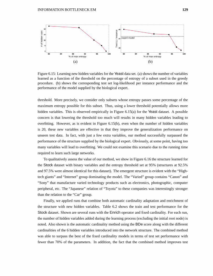
INFORMATION BOTTLENECK EM 129
80 84 88 92 96 10080 84 88 92 96 100
2
6
10
14
18
2
6
10
14
18
% of max entropy
# of
hid
den
vars
80 84 88 92 96 10080 84 88 92 96 100
-49
-47
-45
-49
-47
-45
% of max entropy
Tes
t LL
/ ins
tanc
e
expert model
(a) (b)
Figure 6.15: Learning new hidden variables for the Yeast data set. (a) shows the number of variableslearned as a function of the threshold on the percentage of entropy of a subset used in the greedyprocedure. (b) shows the corresponding test set log-likelihood per instance performance and theperformance of the model supplied by the biological expert.
threshold. More precisely, we consider only subsets whose entropy passes some percentage of the
maximum entropy possible for this subset. Thus, using a lower threshold potentially allows more
hidden variables. This is observed empirically in Figure 6.15(a) for the Yeast dataset. A possible
concern is that lowering the threshold too much will results in many hidden variables leading to
overfitting. However, as is evident in Figure 6.15(b), even when the number of hidden variables
is 20, these new variables are effective in that they improve the generalization performance on
unseen test data. In fact, with just a few extra variables, our method successfully surpassed the
performance of the structure supplied by the biological expert. Obviously, at some point, having too
many variables will lead to overfitting. We could not examine this scenario due to the running time
required to learn such large networks.
To qualitatively assess the value of our method, we show in Figure 6.16 the structure learned for
the Stock dataset with binary variables and the entropy threshold set at 95% (structures at 92.5%
and 97.5% were almost identical for this dataset). The emergent structure is evident with the “High-
tech giants” and “Internet” group dominating the model. The “Varied” group contains “Canon” and
“Sony” that manufacture varied technology products such as electronics, photographic, computer
peripheral, etc. The “Japanese” relation of “Toyota” to these companies was interestingly stronger
than the relation to the “Car” group.
Finally, we applied runs that combine both automatic cardinality adaptation and enrichment of
the structure with new hidden variables. Table 6.2 shows the train and test performance for the
Stock dataset. Shown are several runs with the Enrich operator and fixed cardinality. For each run,
the number of hidden variables added during the learning process (excluding the initial root node) is
noted. Also shown is the automatic cardinality method using the BDe score along with the different
cardinalities of the 6 hidden variables introduced into the network structure. The combined method
was able to surpass the best of the fixed cardinality models in terms of test set performance with
fewer than 70% of the parameters. In addition, the fact that the combined method improves test

130 INFORMATION BOTTLENECK EM
Internet
T2
AOL
Cisco
Intel
T0
T1
Varied
High-tech giants
Yahoo Amazon
InfoSeek
Netscape
Nissan GatewayMicrosoft
3COM DellCompaq
AMDMotorola
GM
Ford
Cannon
Sony Toyota
Cannon
Sony ToyotaT4T3
Cars
Figure 6.16: Structure learned for the Stock dataset using the enrichment operator augmented withstructure search that use the replace-parent operator. All the hidden variables (circles) are binaryand the subset entropy threshold was set at 95%. The children of each leaf are annotated with aplausible interpretation.
performance but has worse training likelihood, demonstrates its ability to avoid overfitting.
6.12 Related Work
To define the IB-EM algorithm, we introduced a formal relation between the Information Bottleneck
(IB) target Lagrangian and the EM functional. This allowed us to formulate an information-theoretic
regularization for our learning problem. Given this objective, we used two central ideas to make
learning feasible. First, following all annealing methods, we slowly diminish the level of “pertur-
bation” as a way to reach a solution of the hard objective. Second, we use continuation to define a
stable traversal from an easy problem to our goal problem.
A multitude of regularization forms are used in machine learning, typically depending on the
specific form of the target function (see Bishop [1995] and references within). Information-theoretic
regularization has been used for classification with partially labeled data by Szummer and Jaakkola
[2002] and for general scenarios in Deterministic annealing [Rose, 1998].
Of the annealing methods, the well known Simulated annealing [Kirkpatrick et al., 1983] is
least similar to ours. Rather than changing the form of the objective function, Simulated annealing
allows the search procedure to make “downhill” moves with some diminishing probability. This

INFORMATION BOTTLENECK EM 131
Log-likelihood # of # ofCardinality Train Test hiddens parameters2 -19.62 -19.62 5 893 -19.32 -19.37 5 1465 -18.87 -19.04 6 30410 -18.53 -18.96 5 76920 -18.43 -18.98 5 2340BDe (9,6,7,7,7,7) -18.65 -18.94 6 526
Table 6.2: Effect of cardinality when inserting new hidden variables into the network structure withthe Enrich operator for the Stock dataset. A 95% entropy threshold was used for the hidden variablediscovery algorithm. The table shows results for several fixed cardinalities as well as the automaticcardinality method using the BDe score. Shown is the log-likelihood per instance for training aswell as test data, the number of hidden variables and the number of parameters in the model. Forthe automatic method, the cardinalities of each hidden variable is noted.
changes the way the procedure traverses the search space and allows it to potentially reach pre-
viously unattainable solutions. Several papers [Heckerman et al., 1994, Chickering, 1996b, Elidan
et al., 2002] have shown that Simulated annealing is not effective when learning Bayesian networks.
Weight annealing [Elidan et al., 2002], on the other hand, skews the target function directly by
perturbing the weights of instances in diminishing magnitudes. Thus, like our method it changes
the form of Q directly but does not use an information-theoretic regularization. Weight annealing
can actually be applied to a wider variety of problems than our method, including structure search
with complete data. However, like other annealing methods, it requires a cooling scheme. For the
large problems with hidden variables we explored in this paper, Weight annealing proved inferior
with similar running times, and impractical with the settings of Elidan et al. [2002].
Finally, like our method, Deterministic annealing [Rose, 1998] alters the problem by explicitly
introducing an information-theoretic regularization term. Specifically, following the widely recog-
nized maximum entropy principle [Jaynes, 1957], deterministic annealing penalizes the objective
with a term that is the entropy of the model. A concrete application of deterministic annealing to
graphical models was suggested by Ueda and Nakano [1998]. However, when learning graphical
models, the deterministic annealing was not found to be superior to standard EM (e.g., [Smith and
Eisner, 2004]).2 In particular, Whiley and Titterington [2002], Smith and Eisner [2004]) show why
applying deterministic annealing to standard unsupervised learning of Bayesian networks with hid-
den variables is problematic. One possible explanation for why our method works well for these
methods is the difference in motivation of the regularization term. Specifically, our term was moti-
vated by the need for generalization where one want to compress the identity of specific instances.
2Smith and Eisner [2004] also suggest a variant of the deterministic annealing algorithm that appears to work wellbut is only applicable in the context of semi-supervised learning or when an initial informed starting point for the EMalgorithm is at hand.

132 INFORMATION BOTTLENECK EM
Another important difference between the two methods is that, like Weight annealing, deterministic
annealing requires the specification of a cooling policy which makes it potentially impractical for
large generative problems. This problem may be avoided using a method similar to the one we used
in this work. We leave this prospect as well as the challenge of better understanding the relation
between the entropy and information regularization terms for future study.
Continuation methods are a well developed field in mathematics [Watson, 2000]. While these
methods are used extensively and successfully to solve practical engineering challenges such as
complex polynomial systems, they have not been frequently used in machine learning. Recently,
Corduneanu and Jaakkola [2002] used continuation to determine a beneficial balance between la-
beled and unlabeled data. To our knowledge this is the first work in learning graphical models to
use continuation to traverse from an easy solution to the desired maximum likelihood problem.
A complementary aspect of our work is the introduction of modification operators for hidden
variables. Our method both for learning the cardinality of a hidden variable, and for introducing
new hidden variables into the network structure, relies on the annealing process and utilizes emer-
gent signals. The problem of evaluating the cardinality of a hidden variable in a graphical model
was explored in several works (e.g., Chang and Fung [1990], Elidan and Friedman [2001]). The
work of Stolcke and Omohundro [1993] for HMMs was the first to use evaluation of pairwise state
merges to determine adapt the cardinality. In Elidan and Friedman [2001], we extend their method
for general Bayesian networks, and Slonim et al. [2002] used a similar approach within the Infor-
mation Bottleneck framework. All of these methods start with a large number of states, and then
apply bottom-up agglomeration to merge overlaps in the state space and reduce redundancies. By
contrast, our method is able to take an “add-when-needed” approach and state mergers are evaluated
not to collapse states but rather to determine if a new one is needed. Several papers also explored
methods for introducing new hidden variables into the network structure, either for specific classes
of Bayesian networks (e.g., Martin and VanLehn [1995], Spirtes et al. [1993], Zhang [2004]) or
for general models using a structural signature approach [Elidan et al., 2001]. Our contribution in
enriching the structure with new hidden variables is twofold. First, we suggested a natural informa-
tion signature as a “cue” for the presence of a hidden variable. Unlike the structural signature this
signature is flexible and is able to weight the influence of different child nodes. Second, we use the
enrichment approach in conjunction with the continuation approach for bypassing local maxima.
As in cardinality learning, we are able to utilize emergent signals allowing the introduction of new
hidden variables into simpler models rendering them more effective.
6.13 Discussion and Future Work
In this chapter we addressed the challenge of learning models with hidden variables in real-life
scenarios. We presented a general approach for learning the parameters of hidden variables in

INFORMATION BOTTLENECK EM 133
Bayesian networks and introduced model selection operators that allow learning of new hidden
variables and their cardinality. We showed that the method achieves significant improvement on
challenging real-life problems.
The contribution of this chapter is threefold. First, we made a formal connection between the
objective functionals of the Information Bottleneck framework [Tishby et al., 1999, Friedman et al.,
2001] and maximum likelihood learning for graphical models. The Information Bottleneck and
its extensions are originally viewed as methods to understand the structure of a distribution. We
showed that in some sense the Information Bottleneck and maximum likelihood estimation are two
sides of the same coin. The Information Bottleneck focuses on the distribution of variables in each
instance, while maximum likelihood focuses on the projection of this distribution on the estimated
model. This understanding extends to general Bayesian networks the recent results of Slonim and
Weiss [2002] that relate the original Information Bottleneck and maximum likelihood estimation in
univariate mixture distributions.
Second, the introduction of the IB-EM principle allowed us to use an approach that starts with
a solution at γ = 0 and progresses toward a solution in the more complex landscape of γ = 1. This
general scheme is common in Deterministic annealing approaches [Rose, 1998, Ueda and Nakano,
1998]. These approaches “flatten” the posterior landscape by raising the likelihood to the power of
γ. The main technical difference of our approach is the introduction of a regularization term that
is derived from the structure of the approximation of the probability of the latent variables in each
instance. This was combined with a continuation method for traversing the path from the trivial
solution at γ = 0 to a solution at γ = 1. Unlike standard approaches in Deterministic annealing
and Information Bottleneck, our procedure can automatically detect important regions where the
solution changes drastically and ensure that they are tracked closely. In preliminary experiment the
continuation method was clearly superior to standard annealing strategies.
Third, we introduced model enrichment operators for inserting new hidden variables into the
network structure and adapting their cardinality. These operators were specifically geared toward
utilizing the emergent cues resulting from the annealing procedure. This resulted in models that
generalize better and achieve equivalent or better results with a relatively simple model.
The methods presented here can be extended in several directions. First, we can improve the
introduction of new hidden variables into the structure by formulating better “signals” that can be
efficiently calculated for larger clusters. Second, we can use alternative variational approximations
as well as adaptive approximation during the learning process. Third, we want to explore methods
for stopping at γ < 1 as an alternative way for improving generalization performance.

Chapter 7
The “Ideal Parent” method for
Continuous Variable Networks
Up until now, we were mostly concerned with learning new hidden variables and coping with the
difficulties of attaining a favorable model in the presence of multiple local maxima. In real-life do-
mains, we might have to start by facing the more fundamental problem of computational complexity.
This is particularly true when learning networks with continuous variables and varied conditional
probability distributions, which are being used in a wide range of applications, including fault de-
tection (e.g., [U. Lerner and Koller, 2000]), modeling of biological systems (e.g., [Friedman et al.,
2000]) and medical diagnosis (e.g., [Shwe et al., 1991]). Just as in Chapter 6 we addressed the prob-
lem on learning hidden variables in conjunction with the problem of local maxima, in this chapter
we address the problem of hidden variables in conjunction with the problem of computational com-
plexity, when applied to networks with continuous variables.
When learning probabilistic graphical models, the task of structure learning is particularly de-
manding. As discussed in Chapter 2, this task is typically treated as a combinatorial optimization
problem. This problem is typically addressed by heuristic search procedures, such as greedy hill
climbing, that traverses the space of candidate structure. Even this greedy approach can be ex-
tremely time consuming due to the time required to score each candidate structure, particularly in
the presence of missing data or hidden variables. The situation can be even more acute if we want
to learn networks with continuous variables: If we limit ourselves to networks with linear Gaussian
conditional probability distributions [Geiger and Heckerman, 1994], we can use sufficient statis-
tics to summarize the data, as is the case for discrete variables, and use a closed form equation to
evaluate the score of candidate families. In general, however, we are also interested in non-linear
interactions. These do not have sufficient statistics, and require costly parameter optimization to
evaluate the score of a candidate family. These difficulties severely limit the applicability of stan-
dard heuristic structure search procedures to rich non-linear models.
134

THE “IDEAL PARENT” METHOD FOR CONTINUOUS VARIABLE NETWORKS 135
We present a general method for speeding search algorithms for structure learning in continuous
variable networks. Our method can be applied to many forms of a unimodal parametric conditional
distribution, including the linear Gaussian model as well as many non-linear models. The ideas
are inspired from the notion of residues in regression [McCullagh and Nelder, 1989], and involve
the notion of “ideal parents”. For each variable, we construct an ideal parent profile of a new
hypothetical parent that would lead to the best possible prediction of the variable. We then use
this profile to efficiently select potential candidate parents that have a similar profile of values.
Using basic principles, we derive a similarity measure that can be computed efficiently and that
approximates the improvement in score that will result from the addition of a candidate parent.
This provides us with a fast method for scanning many potential parents and focus more careful
evaluation (exact scoring) to a smaller number of promising candidates.
The ideal parent profiles we construct during search also provide new leverage on the problem
of introducing new hidden variables during structure learning. Basically, if the ideal parent profiles
of several variables are sufficiently similar, and are not similar to one of their current parents, we
can consider adding a new hidden parents for all these variables. The ideal profile allows us to
estimate the impact this new variable will have on the score, and suggest the values it takes in each
instance. Thus, our method provides a guided approach for introducing new variables during search,
and allows to contrast this with alternative search steps in a computationally efficient manner.
7.1 The “Ideal parent” Concept
We start with the task of speeding up the structure search algorithm for a Bayesian network with
continuous variables. The complexity of any such algorithm is rooted in the need to score each
candidate structure change, which in turn may require non-linear parameter optimization. Thus,
we want to somehow efficiently approximate the benefit of each candidate and score only the most
promising of these. The manner in which this will help us to discover new hidden variables will
become evident in Section 7.3.
7.1.1 Basic Framework
Consider adding Z as a new parent of X whose current parents in the network are U. Given a
training data D of M instances, to evaluate the change in score, when using the BIC score (see
Section 2.3.2), we need to compute the change in the log-likelihood (see Section 2.2.1)
∆X|U(Z) = `X(U ∪ {Z}, θ′ : D)− `X(U, θ : D) (7.1)
where θ are the current maximum likelihood parameters for the family of X , and θ ′ are the maxi-
mum likelihood parameters after the addition of Z . The change in the BIC score is this difference

136 THE “IDEAL PARENT” METHOD FOR CONTINUOUS VARIABLE NETWORKS
combined with the change in the model complexity penalty terms. Thus, to evaluate this difference,
we need to compute the maximum likelihood parameters X given the new choice of parents. Our
goal is to speed up this computation.
The basic idea of our method is straightforward — for a given variable, we want to construct
a hypothetical “ideal parent” Y that would best predict the variable. We will then compare each
existing candidate parent Z to this imaginary one using a similarity measure C(~y, ~z) (which we
instantiate below) and fully score only the most promising candidates. In order for this approach
to be beneficial, we will want the similarity score to approximate the actual change in likelihood
defined in Eq. (7.1).
Conditional Probability Distribution
To make our discussion concrete, we focus on networks where we represent X as a function of its
parents U = {U1, . . . , Uk} with a conditional probability distribution (CPD) that has the following
general form:
X = g(α1u1, . . . , αkuk : θ) + ε (7.2)
where g is a link function that integrates the contributions of the parents with additional parameters
θ, αi that are scale parameters applied to each of the parents, and ε that is a noise random variable
with zero mean. In here, we assume that ε is Gaussian with variance σ2.
When the function g is the sum of its arguments, this CPD is the standard linear Gaussian CPD.
However, we can also consider non-linear choices of g. For example,
g(α1u1, . . . , αkuk : θ) ≡ θ11
1 + e−P
i αiui+ θ0 (7.3)
is a sigmoid function where the response of X to its parents’ values is saturated when the sum is far
from zero.
Likelihood Function
Given the above form of CPDs, we can now write a concrete form of the log-likelihood function
`X(U, θ : D) =−1
2
M∑
m=1
[log(2π) + log(σ2) +
1
σ2(x[m]− g(u[m]))2
]
=−1
2
[M log(2π) + M log(σ2) +
1
σ2
∑
m
(x[m]− g(u[m]))2
]
where, for simplicity, we absorbed each coefficient αj into each value of uj [m]. Similarly, when
the new parent Z is added with coefficient αz , the new likelihood is
`X(U ∪ {Z}, θ′ : D) = −1
2
[M log(2π) + M log(σ2
z) +1
σ2z
∑
m
(x[m]− g(u[m], αzz[m]))2
]

THE “IDEAL PARENT” METHOD FOR CONTINUOUS VARIABLE NETWORKS 137
Consequently, the difference in likelihood of Eq. (7.1) takes the form of
∆X|U(Z) =−M
2
[log σ2
z − log σ2]
−1
2
[1
σ2z
∑
m
(x[m]− g(u[m], αzz[m]))2 −1
σ2
∑
m
(x[m]− g(u[m]))2
](7.4)
The “Ideal Parent”
We now define the ideal parent for X
Definition 7.1.1: Given a dataset D, and a CPD for X given its parents U, with a link function g
and parameters θ and α, the ideal parent Y of X is such that for each instance m,
x[m] = g(α1u1[m], . . . , αkuk[m], y[m] : θ) (7.5)
Under mild conditions, the ideal parent profile (i.e., value of Y in each instance) can be computed
for almost any unimodal parametric conditional distribution. The only requirement from g is that it
should be invertible w.r.t. each one of the parents. Note that in this definition, we implicitly assume
that x[m] lies in the image of g. If this is not the case, we can substitute x[m] with xg[m], the point
in g’s image closest to x[m]. This guarantees that the prediction’s mode for the current set of parents
and parameters is as close as possible to X .
The resulting profile for the hypothetical ideal parent Y is the optimal set of values for the
k + 1’th parent, in the sense that it would maximize the likelihood of the child variable X . This is
true since by definition, X is equal to the mode of the function of its parents defined by g. Intuitively,
if we can efficiently find a candidate parent Z that is similar to the hypothetically optimal parent,
we can improve the model by adding an edge from this parent to X . We are now ready to instantiate
the similarity measure C(~y, ~z). Below, we demonstrate how this is done for the case of a linear
Gaussian CPD. We extend the framework for non-linear CPDs in Section 7.5.
7.1.2 Linear Gaussian
Let X be a variable in the network with a set of parents U, and a linear Gaussian conditional
distribution. In this case, g in Eq. (7.2) takes the form
g(α1u1, . . . , αkuk : θ) ≡∑
i
αiui + θ0
To choose promising candidate parents for X , we start by computing the ideal parent Y for X given
its current set of parents. This is done by inverting the linear link function g with respect to this

138 THE “IDEAL PARENT” METHOD FOR CONTINUOUS VARIABLE NETWORKS
additional parent Y (note that we can assume, without loss of generality, that the scale parameter of
this additional parent is 1). This results in
y[m] = x[m]−∑
j
αjuj[m]− θ0 (7.6)
We can summarize this in vector notation, by using ~x = 〈x[1], . . . , x[M ]〉, and so we get
~y = ~x− U~α
where U is the matrix of parent values on all instances, and ~α is the vector of scale parameters.
Having computed the ideal parent profile, we now want to efficiently evaluate its similarity to
the profile of candidate parents. Intuitively, we want the similarity measure to reflect the likelihood
gain by adding Z as a parent of X . Ideally, we want to evaluate ∆X|U(Z) for each candidate parent
Z . However, instead of reestimating all the parameters of the CPD after adding Z as a parent, we
approximate this difference by only fitting the scaling factor associated with the new parent and
freezing all other parameters of the CPD (the coefficient parameters of the current parents U and
the variance parameter σ).
Theorem 7.1.2 Suppose that X has parents U with a set ~α of scaling factors. Let Y be the ideal
parent as described above, and Z be some candidate parent. Then the change in the log-likelihood
of X in the data, when adding Z as a parent of X , while freezing all parameters except the scaling
factor of Z , is
C1(~y, ~z)≡maxαZ
`X(U ∪ {Z}, θ ∪ {αZ} : D)− `X(U, θ : D)
=1
2σ2
(~y · ~z)2
~z · ~z
Proof: In the linear Gaussian case y[m] = x[m] − g(u[m]) by definition and g(u[m], αzz[m]) =
g(u[m]) + αzz[m] so that Eq. (7.4) can be written as
∆X|U(Z) =−M
2
[log σ2
z − log σ2]−
1
2
[1
σ2z
∑
m
(y[m]− αzz[m])2 −1
σ2
∑
m
y[m]2
]
=−M
2
[log σ2
z − log σ2]−
1
2
[1
σ2z
(~y · ~y − 2αz~z · ~y + α2
z~z · ~z)−
1
σ2~y · ~y
](7.7)
Since σz = σ this reduces to
∆X|U(Z : αz)≡ `X(U ∪ {Z}, θ ∪ {αZ} : D)− `X(U, θ : D)
=−1
2σ2
(−2αz~z · ~y + α2
z~z · ~z)
(7.8)

THE “IDEAL PARENT” METHOD FOR CONTINUOUS VARIABLE NETWORKS 139
To optimize our only free parameter αz, we use
∂∆X|U(Z : αz)
∂αz= −
1
2σ2(−2~z · ~y + 2αz~z · ~z) = 0 ⇒ αz =
~z · ~y
~z · ~z
Plugging this into Eq. (7.8), we get
C1(~y, ~z)≡maxαz
∆X|U(Z : αz)
=−1
2σ2
(−2
~z · ~y
~z · ~z~z · ~y +
(~z · ~y
~z · ~z
)2
~z · ~z
)
=1
2σ2
(~z · ~y)2
~z · ~z
The form of the similarity measure can be even further simplified
Proposition 7.1.3 Let C1(~y, ~z) be as defined above and let σ be the maximum likelihood parameter
before Z is added as a new parent of X . Then
C1(~y, ~z) =M
2
(~y · ~z)2
(~z · ~z)(~y · ~y)=
M
2cos2 φ~y,~z
where φ~y,~z is the angle between the ideal parent profile vector ~y and the candidate parent profile
vector ~z.
Proof: To recover the maximum likelihood parameter of σ we differentiate the log-likelihood func-
tion as written in Eq. (7.4)
∂`X(U, θ : D)
∂σ2= −
M
2σ2+
1
σ4
∑
m
(x[m]− g(u[m]))2 = 0
⇒ σ2 =1
M
∑
m
(x[m]− g(u[m]))2 =1
M~y · ~y
where the last equality follows from the definition of ~y. The result follows immediately by plugging
this into Theorem 7.1.2 and the fact that cos2 φ~y,~z ≡(~y·~z)2
(~z·~z)(~y·~y)
Thus, there is an intuitive geometric interpretation to the measure C1(~y, ~z): we prefer a profile ~z
that is similar to the ideal parent profile ~y, regardless of its norm: It can easily be shown that ~z = c~y
(for any constant c) maximizes this similarity measure. We retain the less intuitive form of C1(~y, ~z)
in Theorem 7.1.2 for compatibility with later developments.
Note that, by definition, C1(~y, ~z) is a lower bound on ∆X|U(Z), the improvement on the log-
likelihood by adding Z as a parent of X: When we add the parent we optimize all the parameters,
and so we expect to attain a likelihood as high, or higher, than the one we attain by freezing some
of the parameters. This is illustrated in Figure 7.1(a) that plots the true likelihood improvement

140 THE “IDEAL PARENT” METHOD FOR CONTINUOUS VARIABLE NETWORKS
0 20 40 60 80 100 120 140 160 180 2000
20
40
60
80
100
120
140
160
180
200
Sim
ilarit
y
∆ Score0 20 40 60 80 100 120 140 160 180 200
0
20
40
60
80
100
120
140
160
180
200
Sim
ilarit
y
∆ Score
(a) (b)
Figure 7.1: Demonstration of the (a) C1 and (b) C2 bounds for linear Gaussian CPDs. The x-axisis the true change in score as a result of an edge modification. The y-axis is the lower bound of thisscore. Points shown correspond to several thousand edge modifications in a run of the ideal parentmethod on real-life Yeast gene expressions data.
vs. C1 for several thousand edge modifications taken from an experiment using real life Yeast gene
expression data (see Section 7.6).
We can get a better lower bound by optimizing additional parameters. In particular, after adding
a new parent, the errors in predictions change, and so we can readjust the variance term. As it turns
out, we can perform this readjustment in closed form.
Theorem 7.1.4 Suppose that X has parents U with a set ~α of scaling factors. Let Y be the ideal
parent as described above, and Z be some candidate parent. Then the change in the log-likelihood
of X in the data, when adding Z as a parent of X , while freezing all other parameters except the
scaling factor of Z and the variance of X , is
C2(~y, ~z)≡maxαZ ,σ
`X(U ∪ {Z}, θ ∪ {αZ} : D)− `X(U, θ : D)
=−M
2log sin2 φ~y,~z
where φ~y,~z is the angle between ~y and ~z.
Proof: To optimize σz we again consider Eq. (7.4) and set
∂∆X|U(Z)
∂σz= −
M
σz+
1
σ3z
[~y · ~y − 2αz~z · ~y + α2
z~z · ~z]
= 0
Solving for σz and plugging the maximum likelihood parameter αz from the development of C1(~y, ~z),

THE “IDEAL PARENT” METHOD FOR CONTINUOUS VARIABLE NETWORKS 141
we get
σ2z =
1
M
[~y · ~y − 2αz~z · ~y + α2
z~z · ~z]
=1
M
[~y · ~y −
(~z · ~y)2
~z · ~z
]
As we have shown above σ = 1M ~y · ~y and similarly the variance term σ2
z “absorbs” the sum of
squared errors when optimized. Thus, the second term in Eq. (7.4) becomes zero and we can write
C2(~y, ~z) =−M
2
[log(σ2
z)− log(σ2)]
=M
2log
(~y · ~y
~y · ~y − (~z·~y)2
~z·~z
)=
M
2log
1
1− (~z·~y)2
(~z·~z)(~y·~y)
=
M
2log
(1
1− cos2 φ~y,~z
)
=−M
2log sin2 φ~y,~z
It is important to note that both C1 and C2 are monotonic functions of (~y·~z)2
~z·~z , and so they consistently
rank candidate parents of the same variable. However, when we compare changes that involve
different ideal parents, such as adding a parent to X1 compared to adding a parent to X2, the
ranking by these two measures might differ. And so, C2 can provide better guidance to some search
algorithms since
C1(~y, ~z) ≤ C2(~y, ~z) ≤ ∆X|U(Z)
This that this is true due to the choice of parameters we freeze in each of these measures. Indeed,
Figure 7.1(b) clearly shows that C2 is a tighter bound than C1, particularly for promising candidates.
7.2 Ideal Parents in Search
The technical developments of the previous section show that we can approximate the score of
candidate parents for X by comparing them to the ideal parent Y using the similarity measure. Is
this approximate evaluation useful?
When performing a local heuristic search, at each iteration we have a current candidate structure
and we consider some operations on that structure. These operations might include edge addition,
edge replacement, edge reversal and edge deletion. We can readily use the ideal profiles and similar-
ity measures developed to speed up two of these: edge addition and edge replacement. In a network
with N nodes, there are in the order of O(N 2) possible edge additions, O(E ·N) edge replacement
where E is the number of edges in the model, and only O(E) edge deletions and reversals. Thus
our method can be used to speed up the bulk of edge modifications considered by a typical search
algorithm.
When considering adding an edge Z → X , we use the ideal parent profile for X and compute

142 THE “IDEAL PARENT” METHOD FOR CONTINUOUS VARIABLE NETWORKS
its similarity to Z . We repeat this for every other candidate parent for X . We then compute the
full score only for the K most similar candidates, and insert them (and the associated change in
score) to a queue of potential operations. In a similar way, we can utilize the ideal parent profile
for considering edge replacement for X . Suppose that Ui ∈ U is a parent of X . We can define the
ideal profile for replacing U while freezing all other parameters of the CPD of X .
Definition 7.2.1: Given a dataset D, and a CPD for X given its parents U, with a link function g,
parameters θ and α, the replace ideal parent Y of X and Ui ∈ U is such that for each instance m,
x[m] = g(α1u1[m], . . . , αi−1ui−1, αi+1ui+1, . . . , αkuk[m], y[m] : θ) (7.9)
The rest of the developments of the previous section remain the same. For each current parent of X
we compute a separate ideal profile - one corresponding to replacement of that parent with a new
one. We then use the same policy as above for examining replacement of each one of the parents.
For both operations, we can tradeoff between the accuracy of our evaluations and the speed of
the search, by changing K , the number of candidate changes per family for which we compute a
full score. Using K = 1, we only score the best candidate according to the ideal parent method
ranking, thus achieving the largest speedup, However, since our ranking only approximates the true
score difference, this strategy might miss good candidates. Using higher values of K brings us
closer to the standard search algorithm both in terms of move selection quality but also in terms of
computation time.
In the experiments in Section 7.6, we integrated the changes described above into a greedy hill
climbing heuristic search procedure. This procedure also examines moves that remove an edge
and reverse and edge, which we evaluate in the standard way. The greedy hill climbing procedure
applies the best available move at each iteration (among those that were chosen for full evaluation)
as in Algorithm 1. The ideal parent method is independent of the specifics of the search procedure
and simply pre-selects promising candidates for the search algorithm to consider.
7.3 Adding New Hidden Variables
Somewhat unexpectingly, the “ideal parent” method also offer a natural solution to the difficult
challenge that is in the heart of this thesis - that of detecting new hidden variables. Specifically, the
ideal parent profiles provide a straightforward way to find when and where to add hidden variables
to the domain in continuous variable networks. The intuition is fairly simple: if the ideal parents
of several variables are similar to each other, then we know that a similar input is predictive of all
of them. Moreover, if we do not find a variable in the network that is close to these ideal parents,

THE “IDEAL PARENT” METHOD FOR CONTINUOUS VARIABLE NETWORKS 143
then we can consider adding a new hidden variable that will serve as their combined input, and, in
addition, have an informed initial estimate of its profile.
To introduce a new hidden variable, we would like to require that it will be beneficial for several
children at once. The difference in log-likelihood due to adding a new parent with profile ~z is the
sum of differences between the log-likelihoods of families it is involved in:
∆X1,...,XL(Z) =
L∑
i
∆Xi|Ui(Z)
where we assume, without loss of generality, that the members of the cluster are X1, . . . , XL. To
score the network with Z as a new hidden variable, we also we need to deal with the difference in the
complexity penalty term, and the likelihood of Z variable as a root variable. These terms, however,
can be readily evaluated. The difficulty is in finding the profile ~z that maximizes ∆X1,...,XL(Z).
Using the ideal parent approximation, we can lower bound this improvement by
L∑
i
C1(~yi, ~z) ≡L∑
i
1
2σ2i
(~z · ~yi)2
~z · ~z≤ ∆X1,...,XL
(Z) (7.10)
and so we want to find ~z∗ that maximizes this bound. We will then use this optimized bound as our
approximate cluster score. That is we want to find
~z∗ = arg max~z
∑
i
1
2σ2i
(~z · ~yi)2
~z · ~z≡ arg max
~z
~zTYYT~z
~zT~z(7.11)
where Y is the matrix whose columns are yi/σi. ~z∗ must lie in the column span of Y since any
component orthogonal to this span increases the denominator of the right hand term but leaves the
numerator unchanged, and therefore does not obtain a maximum. We can therefore express the
solution as:~z∗ =
∑
i
viyi
σi= Y~v (7.12)
where ~v is a vector of coefficients. Furthermore, the objective in Eq. (7.11) is known as the Rayleigh
quotient of the matrix YYT and the vector ~z. The optimum of this quotient is achieved when ~z
equals the eigenvector of YYT corresponding to its largest eigenvalue [Wilkinson, 1965]. Thus, to
solve for ~z∗ we want to solve the following eigenvector problem
(YYT )~z∗ = λ~z∗
Note that the dimension of YYT is M (the number of instances), so that, in practice, this problem
cannot be solved directly. However, by plugging in Eq. (7.12), multiplying on the right by Y , and

144 THE “IDEAL PARENT” METHOD FOR CONTINUOUS VARIABLE NETWORKS
defining A ≡ YTY , we get a reduced generalized eigenvector problem 1
AA~v = λA~v
Although this problem can now be solved directly, it can be further simplified by noting that A is
only singular if the residue of observations of two or more variables are linearly dependent along
all of the training instances. In practice, for continuous variables, A is indeed non-singular, and we
can multiply both sides A−1 and end up with a simple eigenvalue problem:
A~v = λ~v
which is numerically simpler and easy to solve as the dimension of A is L, the number of variables
in the cluster, which is typically relatively small. Once we find the L dimensional eigenvector ~v∗
with the largest eigenvalue λ∗, we can express with it the desired parent profile ~z∗.
We can get a better bound of ∆X1,...,XL(Z) if we use C2 similarity rather than C1. Unfortu-
nately, optimizing the profile ~z with respect to this similarity measure is a harder problem that is
not solvable in closed form. Since the goal of the cluster identification is to provide a good starting
point for the following iterations that will eventually adapt the structure, we use the closed form
solution for Eq. (7.11). Note that once we optimized the profile z using the above derivation, we
can still use the C2 similarity score to provide a better bound on the quality of this profile as a new
parent for X1, . . . , XL.
Now that we can approximate the benefit of adding a new hidden parent to a cluster of variables,
we still need to consider different clusters to find the most beneficial one . As the number of clusters
is exponential, we adapt a heuristic agglomerative clustering approach (e.g., [Duda and Hart, 1973])
to explore different clusters. We start with each variable as an individual cluster and repeatedly
merge the two clusters that lead to the best expected improvement in the BIC score (or the least
decrease). This procedure potentially involves O(N 3) merges, where N is the number of possible
variables. We save much of the computations by pre-computing the matrix Y TY only once, and then
using the relevant sub-matrix in each merge. In practice, the time spent in this step is insignificant
in the overall search procedure.
7.4 Learning with Missing Values
Once we add a hidden variable to the network structure, in subsequent structure search, we have to
cope with missing values, even if the original training data was complete. Similar considerations
can arise if the dataset contains partial observations of some of the variables. To deal with this
1In the Generalized Eigenvector Problem, we want to find eigenpairs (λ,~v) so that B~v = λA~v holds.

THE “IDEAL PARENT” METHOD FOR CONTINUOUS VARIABLE NETWORKS 145
problem, we use the Expectation Maximization approach [Dempster et al., 1977] and its application
to network structure learning [Friedman, 1997] (see Section 2.4 for more details).
How can we combine the ideal parent method into this structural EM search? Since we do
not necessarily observe neither X nor all of its parents, the definition of the ideal parent cannot be
applied directly. Instead, we define the ideal parent to be the profile that will match the expectations
given Q. That is, we choose y[m] so that
IEQ[x[m] | Do] = IEQ[g(α1u1[m], . . . , αkuk[m], y[m] : θ) | Do]
In the case of linear CPDs, this implies that
~y = IEQ[~x | Do]− IEQ[U | Do]~α
Once we define the ideal parent, we can use it to approximate changes in the expected BIC score
(given Q). For the case of a linear Gaussian, we get terms that are similar to C1 and C2 of Theo-
rem 7.1.2 and Theorem 7.1.4, respectively. The only change is that we apply the similarity measure
on the expected value of ~z for each candidate parent Z . This is in contrast to exact evaluation of
IEQ
[∆X|UZ | Do
], which requires the computation of the expected sufficient statistics of U, X ,
and Z . To facilitate efficient computation, we adopt an approximate variational mean-field form
(e.g., [Jordan et al., 1998, Murphy and Weiss, 1999]) for the posterior. This approximation is used
both for the ideal parent method and the standard greedy approach used in Section 7.6. This results
in computations that require only the first and second moments for each instance z[m], and thus can
be easily obtained from Q.
Finally, we note that the structural EM iterations are still guaranteed to converge to a local
maximum. In fact, this does not depend on the fact that C1 and C2 are lower bounds of the true
change to the score, since these measures are only used to pre-select promising candidates which are
scored before actually being considered by the search algorithm. Indeed, the ideal parent method
is a modular structure candidate selection algorithm and can be used as a black-box by any search
algorithm.
7.5 Non-linear CPDs
We now address the important challenge of non-linear CPDs. In the class of CPDs we are consid-
ering, this non-linearity is mediated by the link function g, which we assume here to be invertible.
Examples of such functions include the sigmoid function shown in Eq. (7.3) and hyperbolic func-
tions that are suitable for modeling gene transcription regulation [Nachman et al., 2004], among
many others. When we learn with non-linear CPDs, parameter estimation is harder. To evaluate a
potential parent P for X we have to perform non-linear optimization (e.g., conjugate gradient) of all

146 THE “IDEAL PARENT” METHOD FOR CONTINUOUS VARIABLE NETWORKS
of the α coefficients of all parents as well as other parameters of g. In this case, a fast approximation
can boost the computational cost of the search significantly.
As in the case of linear CPDs, we compute the ideal parent profile ~y by inverting g. (We assume
that the inversion of g can be performed in time that is proportional to the calculation of g itself as
is the case for the CPDs considered above.) Suppose we are considering the addition of a parent to
X in addition to its current parents U, and that we have computed the value of the ideal parent y[m]
for each sample m by inversion of g. Now consider a particular candidate parent Z whose value
at the m’th instance is Z[m]. How will the difference between the ideal value and the value of Z
reflect in prediction of X for this instance?
As we have seen in Section 7.1, in the linear case, the difference z[m]−y[m] translated through
g to a prediction error. In the non-linear case, the effect of the difference on predicting X depends on
other factors, such as the values of the other parents. To see this, consider again the sigmoid function
g of Eq. (7.3). If the sum of the arguments to g is close to 0, then g locally behaves like a sum of
its arguments. On the other hand, if the sum is far from 0, the function is in one of the saturated
regions, and big differences in the input almost do not change the prediction. This complicates our
computations and does not allow the development of similarity measures as in Theorem 7.1.2 and
Theorem 7.1.4 directly.
We circumvent this problem by approximating g with a linear function around the value of the
ideal parent profile. We use a first-order Taylor expansion of g around the value of ~y and write
g(~u, ~z) ≈ g(~u, ~y) + (~z − ~y)∂g(~u, ~y)
∂~y
As a result, the “penalty” for a distance between ~z and ~y depends on the gradient of g at the particular
value of ~y, given the value of the other parents. In instances where the derivative is small, larger
deviations between y[m] and z[m] have little impact on the likelihood of x[m], and in instances
where the derivative is large, the same deviations may lead to worse likelihood.
To understand the effect of this approximation in more detail we consider a simple example
with a sigmoid Gaussian CPD as defined in Eq. (7.3), where X has no parents in the current net-
work and Z is a candidate new parent. Figure 7.2(a) shows the sigmoid function (dotted) and
its linear approximation at Y = 0 (solid) for an instance where X = 0.5. The computation of
Y = log(
10.5 − 1
)= 0 by inversion of g is illustrated by the dashed lines. (b) is the same for a
different sample where X = 0.85. In (c),(d) we can see the effect of the approximation for these
two different samples on our evaluation of the likelihood function. For a given probability value,
the likelihood function is more sensitive to changes in the value of Z around Y when X = 0.5
when compared to the instance X = 0.85. This can be seen more clearly in (e) where equi-potential
contours are plotted for the sum of the approximate log-likelihood of these two instances. To re-
cover the setup where our sensitivity to Z does not depend on the specific instance as in the linear
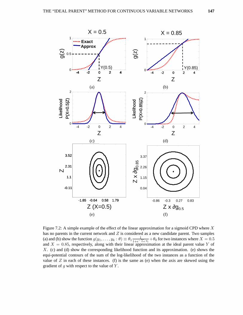
THE “IDEAL PARENT” METHOD FOR CONTINUOUS VARIABLE NETWORKS 147
X = 0.5
g(z)
Y(0.5)
ExactApprox
Z
0
1
0.5
-4 -2 0 2 4-4 -2 0 2 4-4 -2 0 2 4-4 -2 0 2 4
X = 0.85
g(z)
Y(0.85)-4 -2 0 2 4-4 -2 0 2 4
0
1
Z(a) (b)
Z
0
2
-4 -2 0 2 4
Like
lihoo
d
P(X
=0.
5|Z
)
Like
lihoo
d
P(X
=0.
5|Z
)
Z
0
2
-4 -2 0 2 4
P(X
=0.
85|Z
)
Like
lihoo
d
P(X
=0.
85|Z
)
Like
lihoo
d
(c) (d)
-1.85 -0.64 0.58 1.79-1.85 -0.64 0.58 1.79
-0.11
1.1
2.31
3.52
-0.11
1.1
2.31
3.52
Z (X=0.5)
Z
-0.86 -0.3 0.27 0.83
0.04
1.15
2.26
3.37
Z x ∂g0.5
Z x
∂g 0
.85
(e) (f)
Figure 7.2: A simple example of the effect of the linear approximation for a sigmoid CPD where Xhas no parents in the current network and Z is considered as a new candidate parent. Two samples(a) and (b) show the function g(y1, . . . , yk : θ) ≡ θ1
11+e−
P
i yi+θ0 for two instances where X = 0.5
and X = 0.85, respectively, along with their linear approximation at the ideal parent value Y ofX . (c) and (d) show the corresponding likelihood function and its approximation. (e) shows theequi-potential contours of the sum of the log-likelihood of the two instances as a function of thevalue of Z in each of these instances. (f) is the same as (e) when the axis are skewed using thegradient of g with respect to the value of Y .

148 THE “IDEAL PARENT” METHOD FOR CONTINUOUS VARIABLE NETWORKS
case, we consider a skewed version of Z · ∂g/∂y rather than Z directly. The result is shown in
Figure 7.2(f). We can generalize the example above to develop a similarity measure for the general
non-linear case
Theorem 7.5.1 Suppose that X has parents U with a set ~α of scaling factors. Let Y be the ideal
parent as described above, and Z be some candidate parent. Then the change in log-likelihood of X
in the data, when adding P as a parent of X , while freezing all other parameters, is approximately
C1(~y ◦ g′(~y), ~z ◦ g′(~y))−1
2σ2(k1 − k2). (7.13)
where g′(~y) is the vector whose m’th component is ∂g(~αu, y)/∂y |~u[m],y[m], and ◦ denotes component-
wise product. Similarly, if we also optimize the variance, then the change in log-likelihood is ap-
proximately
C2(~y ◦ g′(~y), ~z ◦ g′(~y))−M
2log
k1
k2(7.14)
In both cases,
k1 = (~y ◦ g′(~y)) · (~y ◦ g′(~y)) ; k2 = (~x− g(~u)) · (~x− g(~u))
do not depend on ~z.
Thus, we can use exactly the same measures as before, except that we “distort” the geometry with
the weight vector g′(y) that determines the importance of different instances. To approximate the
likelihood difference, we also add the correction term which is a function of k1 and k2. This cor-
rection is not necessary when comparing two candidates for the same family, but is required for
comparing candidates from different families, or when adding hidden values. Note that unlike the
linear case, our theorem now is approximate by definition due to the linear approximation of g.
Proof: Using the general form of the Taylor linear approximation for a non-linear link function g,
Eq. (7.4) can be written as
∆X|U(Z)
≈−M
2log
σ2z
σ2−
1
2
[1
σ2z
[~x− g(~u, ~y)− (αz~z − ~y) ◦ ∂g]2 −1
σ2[~x− g(~u)]2
]
=−M
2log
σ2z
σ2−
1
2σ2z
[α2
z(~z ◦ ∂g)2 − 2αz(~z ◦ ∂g) · (~y ◦ ∂g) + (~y∂g)2]+
1
2σ2[~x− g(~u)]2
=−M
2log
σ2z
σ2−
1
2σ2z
[α2
z~z? · ~z? − 2αz~z? · ~y? + ~y? · ~y?
]+
1
2σ2[~x− g(u)]2 (7.15)
where we use the fact that ~x−g(~u, ~y) = 0 by construction of ~y, and we denote for clarity ~y? ≡ ~y◦∂g

THE “IDEAL PARENT” METHOD FOR CONTINUOUS VARIABLE NETWORKS 149
and ~z? ≡ ~z ◦ ∂g. To optimize αz we use
∂∆X|U(Z)
∂αz≈ −
1
2σ[2αz~z? · ~z? − 2~z? · ~y?] ⇒ αz =
~z? · ~y?
~z? · ~z?
Plugging this into Eq. (7.15) we get
∆X|U(Z)≈1
2σ2
(~z? · ~y?)2
~z? · ~z?−
1
2σ2~y? · ~y? +
1
2σ2[~x− g(~u)]2
= C1(~y?, ~z?)−1
2σ2(k1 − k2)
which proves Eq. (7.13). When we also optimize that variance, as noted before, the variance terms
absorbs the sum of squared errors, so that
σz =1
M
[~y? · ~y? −
(~z? · ~y?)2
~z? · ~z?
]
Plugging this into Eq. (7.15) results in
∆X|U(Z)≈−M
2log
σ2
σ2z
=M
2log
[~x− g(u)]2
~y? · ~y? −(~z?·~y?)2
~z?·~z?
=M
2log
[~x− g(u)]2
~y? · ~y?
[1− (~z?·~y?)2
~z?·~z?~y?·~y?
]
=M
2log
1
1− (~z?·~y?)2
~z?·~z?~y?·~y?
+M
2log [~x− g(u)]2 −
M
2log(~y? · ~y?)
= C2(~y?, ~z?)−M
2log
k1
k2
As in the linear case, the above theorem allows us to efficiently evaluate promising candidates for
the add edge step in the structure step, and the replace edge step can also be approximated with
minor modifications. As before, the significant gain in speed is that we only perform few parameter
optimizations (that are expected to be costly as the number of parents grows), rather than O(N)
such optimizations.
Adding a new hidden variable with non-linear CPDs introduces further complications. We want
to use, similarly to the case of a linear model, the structure score of Eq. (7.10) with the distorted
C1 measure. Optimizing this measure has no closed form solution in this case and we need to
resort to an iterative procedure or an alternative approximation. We use an approximation where the
correction terms of Eq. (7.13) are omitted so that a form that is similar to the linear Gaussian case
is used, with the “distorted” geometry of ~y. Having made this approximation, the rest of the details

150 THE “IDEAL PARENT” METHOD FOR CONTINUOUS VARIABLE NETWORKS
are the same as in the linear Gaussian case.
7.6 Experiments
We now examine the impact of the ideal parent method in two settings. In the first setting, we use
this method for pruning the number of potential moves that are evaluated by greedy hill climbing
structure search. We apply this learning procedure to complete data (and data with some missing
values) to learn dependencies between the observed variables. In the second setting, we use the
ideal parent method as a way of introducing new hidden variables, and also as a guide to reduce the
number of evaluations when learning structure that involves hidden variables and observed ones,
using a Structural EM search procedure.
In the first setting, we applied standard greedy hill climbing search (Greedy) and greedy hill
climbing supplemented by the ideal parent method as discussed in Section 7.2 (Ideal). In using
the ideal parent method, we used the C2 similarity measure (Section 7.1) to rank candidate edge
additions and replacements, and then applied full scoring only to the top K ranking candidates per
variable.
To evaluate the impact of the method, we start with a synthetic experiment where we know the
true underlying network structure. In this setting we can evaluate the magnitude of the performance
cost that is the result of the approximation we use. (We examine the speedup gain of our method
on more interesting real-life examples below.) We used a network learned from real data (see be-
low) with 44 variables. From this network we can generate datasets of different sizes and apply
our method with different values of K . Figure 7.3 compares the ideal parent method and the stan-
dard greedy procedure for linear Gaussian CPDs (left column) and sigmoid CPDs (right column).
Using K = 5 is, as we expect, closer to the performance of the standard greedy method both in
terms of training set [(a),(e)] and test set [(b),(f)] performance then K = 2. For linear Gaussian
CPDs test performance is essentially the same for both methods. Using sigmoid CPDs we can see
a slight advantage for the standard greedy method. When considering the percent of true edges
recovered [(c),(g)], as before, the standard method shows some advantage over the ideal method
with K = 5. However, by looking at the total number of edges learned [(d),(h)], we can see that the
standard greedy method achieves this by using close to 50% more edges than the original structure
for sigmoid CPDs. Thus, advantage in performance comes at a high complexity price (and as we
demonstrate below, at a significant speed cost).
We now examine the effect of the method on learning from real-life datasets. We base our
datasets on a study that measures the expression of the baker’s yeast genes in 173 experiments
[Gasch et al., 2000]. In this study, researchers measured expression of 6152 yeast genes in its
response to changes in the environmental conditions, resulting in a matrix of 173 × 6152 measure-
ments. In the following, for practical reasons, we use two sets of genes. The first set consists of 639

THE “IDEAL PARENT” METHOD FOR CONTINUOUS VARIABLE NETWORKS 151
100 1000
−1.2
−1.1
−1
Tra
in
GreedyIdeal K=2Ideal K=5Gold
100 1000
−0.6
−0.4
−0.2
0
Tra
in
(a) (e)
100 1000−1.8
−1.6
−1.4
−1.2
−1
−0.8
Tes
t
100 1000−1
−0.8
−0.6
−0.4
−0.2
0
Tes
t
(b) (f)
100 10000
0.2
0.4
0.6
0.8
Rec
all
100 10000
0.2
0.4
0.6
0.8
Rec
all
(c) (g)
100 10000
0.5
1
1.5
To
tal
100 10000
0.5
1
1.5
To
tal
(d) (h)
Figure 7.3: Evaluation of Ideal search on synthetic data generated from a real-life like networkwith 44 variables. We compare Ideal search with K = 2 (dashed) and K = 5 (solid), against thestandard Greedy procedure (dotted). The figures show, as a function of the number of instances(x-axis), for linear Gaussian CPDs: (a) average training log likelihood per instance per variable;(b) same for test; (c) fraction of true edges obtained in learned structure; (d) total number of edgeslearned as fraction of true number of edges. (e)-(h) same for sigmoid CPDs.

152 THE “IDEAL PARENT” METHOD FOR CONTINUOUS VARIABLE NETWORKS
Ideal K = 2 vs Greedy Ideal K = 5 vs GreedyDataset vars inst train test edge move eval sp train test edge move eval sp
Linear Gaussian with complete dataAA 44 173 -0.024 0.006 87.1 96.5 3.6 2 -0.008 0.007 94.9 96.5 9.3 2AA Cond 173 44 -0.038 0.082 92.2 92.6 1.2 2 -0.009 0.029 96.9 98.2 2.9 2Met 89 173 -0.033 -0.024 88.7 91.5 1.6 3 -0.013 -0.016 94.5 96.9 4.4 2Met Cond 173 89 -0.035 -0.015 91.3 98.0 1.0 2 -0.007 -0.023 98.9 98.5 2.4 2
Linear Gaussian with missing valuesAA 354 173 -0.101 -0.034 81.3 95.2 0.4 5 -0.048 -0.022 90.7 96.0 0.9 5AA Cond 173 354 -0.066 -0.037 74.7 87.5 0.4 14 -0.033 -0.021 86.3 101.1 1.6 11
Sigmoid with complete dataAA 44 173 -0.132 -0.065 49.7 59.4 2.0 38 -0.103 -0.046 60.4 77.6 6.1 18AA Cond 173 44 -0.218 0.122 62.3 76.7 1.0 36 -0.150 0.103 73.7 79.4 2.3 21Met 89 173 -0.192 -0.084 47.9 58.3 0.9 65 -0.158 -0.059 56.6 69.8 2.6 29Met Cond 173 89 -0.207 -0.030 60.5 69.5 0.8 53 -0.156 -0.042 69.8 77.7 2.2 29
Table 7.1: Performance comparison of the Ideal parent search with K = 2, K = 5 and Greedy onreal data sets. vars - number of variables in the dataset; inst - the number of instances in the dataset;train - average difference in training set log-likelihood per instance per variable; test - same for testset; edges - percent of edges learned by Ideal with respect to those learned by Greedy. moves - per-cent of structure modifications taken during the search; eval - percent of moves evaluated; speedup- speedup of Ideal over greedy method. All numbers are averages over 5 fold cross validation sets.
genes that participate in general metabolic processes (Met), and the second is a subset of the first
with 354 genes which are specific to amino acid metabolism (AA). We choose these sets since part
of the response of the yeast to changes in its environment is in altering the activity levels of different
parts of its metabolism. For some of the experiments below, we focused on subsets of genes for
which there are no missing values, consisting of 89 and 44 genes, respectively). On these datasets
we can consider two tasks. In the first, we treat genes as variables and experiments as instances. The
learned networks indicate possible regulatory or functional connections between genes [Friedman
et al., 2000]. A complementary task is to treat the 173 experiments as variables (Cond). In this case
the network encodes relationships between different conditions.
In Table 7.1 we summarize differences between the Greedy search and the Ideal search with
K set to 2 and 5, for the linear Gaussian CPDs as well as sigmoid CPDs. Since the C2 similarity
is only a lower bound of the BIC score difference, we expect the candidate ranking of the two
to be different. As most of the difference comes from freezing some of the parameters, a possible
outcome is that the Ideal search is less prone to over-fitting. Indeed as we see, though the training
set log likelihood in most cases is lower for Ideal search, the test set performance is only marginally
different than that of the standard greedy method, and often surpasses it.
Of particular interest is the tradeoff between accuracy and speed when using the ideal parent
method. In Figure 7.4 we examine this tradeoff in four of the data sets described above using linear
Gaussian and sigmoid CPDs. For both types of CPDs, the performance of the ideal parent method
approaches that of Greedy as K is increased. As we can expect, in both types of CPDs the ideal

THE “IDEAL PARENT” METHOD FOR CONTINUOUS VARIABLE NETWORKS 153
0.1
0.2
1 2 3 4 5K
test
∆∆ ∆∆-l
og
-lik
elih
oo
d AminoMetabolismConditions (AA)Conditions (Met)
0
1 2 3 4 5K
0.1
0.2
1 2 3 4 5K
test
∆∆ ∆∆-l
og
-lik
elih
oo
d AminoMetabolismConditions (AA)Conditions (Met)
0
1 2 3 4 5K
0.1
0.2
1 2 3 4 5K
1 2 3 4 5K
test
∆∆ ∆∆-l
og
-lik
elih
oo
d AminoMetabolismConditions (AA)Conditions (Met)
AminoMetabolismConditions (AA)Conditions (Met)
AminoMetabolismConditions (AA)Conditions (Met)
0
1 2 3 4 5K
1 2 3 4 5K
greedy
0
1
2
3
4
spee
du
p
1 2 3 4 5K
0
1
2
3
4
spee
du
p
1 2 3 4 5K
0
1
2
3
4
spee
du
p
1 2 3 4 5K
1 2 3 4 5K
(a) Gaussian performance (b) Gaussian speedup
-0.1
0
0.1
test
∆∆ ∆∆-l
og
-lik
elih
oo
d
0 5 10 15 20K
AminoMetabolismConditions (AA)Conditions (Met)
greedy
-0.1
0
0.1
test
∆∆ ∆∆-l
og
-lik
elih
oo
d
0 5 10 15 20K
-0.1
0
0.1
-0.1
0
0.1
test
∆∆ ∆∆-l
og
-lik
elih
oo
d
0 5 10 15 20K
0 5 10 15 20K
AminoMetabolismConditions (AA)Conditions (Met)
AminoMetabolismConditions (AA)Conditions (Met)
greedy
20
60
100
spee
du
p
0 5 10 15 20K
20
60
100
spee
du
p
0 5 10 15 20K
20
60
100
20
60
100
spee
du
p
0 5 10 15 20K
0 5 10 15 20K
(c) sigmoid performance (d) sigmoid speedup
Figure 7.4: Evaluation of Ideal search on real-life data using 5-fold cross validation. (a) averagedifference in log likelihood per instance on test data when learning with linear Gaussian CPDsrelative to the Greedy baseline (y-axis) vs. the number of ideal candidates for each family K(x-axis). (b) Relative speedup over Greedy (y-axis) against K (x-axis). (c),(d) same for sigmoidCPDs.
parent method is faster even for K = 5. However, the effect on total run time is much more pro-
nounced when learning networks with non-linear CPDs. In this case, most of the computation is
spent in optimizing the parameters for scoring candidates. And so, reducing the number of candi-
dates evaluated results in a dramatic effect. This speedup in non-linear networks makes previously
“intractable” real-life learning problems (like gene regulation network inference) more accessible.
In the second experimental setting, we examine the ability of our algorithm to learn structures
that involve hidden variables and introduce new ones during the search. In this setting, we focus on
two layered networks where the first layer consists of hidden variables, all of which are assumed to
be roots, and the second layer consists of observed variables. Each of the observed variables is a

154 THE “IDEAL PARENT” METHOD FOR CONTINUOUS VARIABLE NETWORKS
(a)
10 100-60
-40
-20
trai
n lo
g-lik
elih
ood
Instances
GreedyIdeal K=2Ideal K=5Gold
GreedyIdeal K=2Ideal K=5Gold
10 100
-100
-60
-20
test
log-
likel
ihoo
d
Instances
GreedyIdeal K=2Ideal K=5Gold
10 100
-100
-60
-20
test
log-
likel
ihoo
d
Instances
GreedyIdeal K=2Ideal K=5Gold
GreedyIdeal K=2Ideal K=5Gold
(b) (c)
Figure 7.5: Evaluation of performance in two-layer network experiments using synthetic data gen-erated from the Gold structure with 141 variables shown in (a), which was curated by a biologicalexpert. (b) average log likelihood per instance on training data (y-axis) for Greedy , Ideal searchwith K = 2 and Ideal search with K = 5, when learning with linear Gaussian CPDs against thenumber of training samples (x-axis). (c) Same for test set.
leaf and can depend on one or more hidden variables. Learning such networks involves introducing
different hidden variables, and determining for each observed variable which hidden variables it
depends on.
To test the performance of our algorithm, we used a network topology that is curated [Nachman
et al., 2004] from biological literature for the regulation of cell-cycle genes in yeast. This network
involves 7 hidden variables and 141 observed variables. We learned the parameters for the network
from a cell cycle gene expression dataset [Spellman et al., 1998]. From the learned network we
then sampled datasets of varying sizes, and tried to recreate the regulation structure using either
greedy search or ideal parent search. In both search procedures we introduce hidden variables in a
gradual manner. We start with a network where a single hidden variable is connected as the only
parent to all observed variables. After parameter optimization, we introduce another hidden variable
- either as a parent of all observed variables (in greedy search), or to members of the highest scoring
cluster (in ideal parent search, as explained in Section 7.3). We then let the structure search modify

THE “IDEAL PARENT” METHOD FOR CONTINUOUS VARIABLE NETWORKS 155
max parents5 2 5 2 5
0
0.1
0.2
0.3
∆te
st lo
g-lo
ss /
inst
ance
/ va
riabl
e
2
Greedy
Full Ideal K=2Greedy + Ideal new varsFull Ideal K=2Greedy + Ideal new varsFull Ideal K=2Greedy + Ideal new vars
AA Sigmoid AA Gaussian AA Cond Gaussian
Figure 7.6: Structure learning of bipartite networks where the parents are new hidden variables andthe children are the observed variables. The different datasets of the baker’s Yeast include: AAwith 44 variables for both Gaussian and sigmoid Gaussian CPDs; AA Cond with 173 variables andGaussian CPDs. For each datasets a structure with up to 2 and 5 parents was considered. Shownare the test log-likelihood per instance per variable relative to the baseline of the standard greedystructure learning algorithm.
edges (subject to the two-layer constraints) until no beneficial moves are found, at which point we
introduce another hidden variable, and so on. The search terminates when it is no longer beneficial
to add a new variable.
Figure 7.5 shows the performance of the ideal parent search and the standard greedy procedure
as a function of the number of instances, for linear Gaussian CPDs. As can be seen, although
there are some differences in training set likelihood, the performance on test data is essentially the
same. Thus, as in the case of the yeast experiments considered above, there was no degradation of
performance due to the approximation made by our method.
We then considered the application of the algorithms to real-life datasets. Figure Figure 7.6
shows the test set results for several of the datasets of the baker’s yeast [Gasch et al., 2000] described
above, for both Gaussian and sigmoid Gaussian CPDs. The full ideal parent method (blue ’+’) with
K = 2 and the ideal method for adding new hidden variables is consistently better than the baseline
greedy procedure. To demonstrate that the improvement is in large part due to the guided method for
adding hidden variables we also ran the baseline greedy procedure for structure changes augmented

156 THE “IDEAL PARENT” METHOD FOR CONTINUOUS VARIABLE NETWORKS
with the ideal method for adding new hidden variables (red ’X’). As can be seen, the performance
of this method is typically slightly better than the full ideal method, since it does not approximate
the structural adaptation stage. In this setup, the only difference from the greedy baseline is the way
that new hidden variables are introduced. Thus, these results support our hypothesis that the ideal
method is able to introduce effective new hidden variables, that are preferable to a hidden variables
that are naively introduced into the network structure.
We also considered the application of our algorithm to the real-life cell-cycle gene expression
data described above with linear Gaussian CPDs. Although this data set contains only 17 samples,
it is of high interest from a biological perspective to try and infer from it as much as possible on
the structure of regulation. We performed leave-one-out cross validation and compared the ideal
parent method with K = 2 and K = 5 to the standard greedy method. To help avoid over-fitting,
we limited the number of hidden parents for each observed variable to 2. In terms of training
log-likelihood per instance per variable, the greedy method is better than the ideal method by 0.4
and 0.42 bits per instance, for K = 5 and K = 2, respectively. However, its test log-likelihood
performance is significantly worse as a result of high over-fitting of two particular instances, and
is worse by 0.72 bits per instance than the ideal method with K = 5 and by 0.88 bits per instance
than the ideal method with K = 2. As we have demonstrated in the synthetic example above, the
ability of the ideal method to avoid over-fitting via a guided search, does not come at the price of
diminished performance when data is more plentiful. When the observed variables were allowed
to have up to 5 parents, all methods demonstrated over-fitting, which for Greedy was by far more
severe.
The superiority of the sigmoid Gaussian over the Gaussian model for the AA dataset (in the
order of 1 bit per instance per variable) motivates us to pursue learning of models with non-linear
CPDs. We could not compare the different methods for the larger datasets as the greedy method did
not complete runs given several days of CPU time. We believe that the ability of the ideal method
to avoid over fitting will only increase its strength in these more challenging cases.
7.7 Discussion and Future Work
In this chapter we set out to learn continuous variable networks with hidden variables. Our con-
tribution is twofold: First, we showed how to speed up structure search, particularly for non-linear
conditional probability distributions. This speedup is essential as it makes structure learning feasi-
ble in many interesting real life problems. Second, we presented a principled way of introducing
new hidden variables into the network structure. We used the concept of an “ideal parent” for both
of these tasks and demonstrated its benefits on both synthetic and real-life biological domains. In
particular, we showed that our method is able to learn new hidden variables that improve the perfor-
mance. In addition, it allowed us to cope with domains where the greedy method proved too time

THE “IDEAL PARENT” METHOD FOR CONTINUOUS VARIABLE NETWORKS 157
consuming.
The unique aspect of the Ideal Parent approach is that it leverages on the parametric structure
of the conditional distributions. In here, we applied this approach in conjunction with a greedy
search algorithm. However, it can also be supplemented to many other search procedures, such as
simulated annealing, as a way of speeding up evaluation of candidate moves. Of particular interest
is how our method can help methods that inherently limit the search to promising candidates such
as the “Sparse Candidate” method of Friedman et al. [1999c].
Both of the CPDs we examined are specific instances of generalized linear models (GLMs)
[McCullagh and Nelder, 1989]. This class of CPDs uses a function g that is applied to the sum of
its arguments, called the link function in the GLM literature. However, we can also consider more
complex functions, as long as they are well defined for any desired number of parents. For example,
in [Nachman et al., 2004] models based on chemical reaction models are considered, where the
function g does not have a GLM form. An example of a two variable function of this type is:
g(y1, y2 : θ) = θy1y2
(1 + y1)(1 + y2)
We also note that GLM literature deals extensively with different forms of noise. While we focus
here on the case of additive Gaussian noise, the ideas we propose here can be extended to many of
these noise distributions.
Few works touched on the issue of when and how to add a hidden variable in the network
structure (e.g., [Elidan et al., 2001, Elidan and Friedman, 2003, Martin and VanLehn, 1995, Zhang,
2004]). Only some of these method are potentially applicable to continuous variable networks, and
none have been adapted to this context. To our knowledge, this is the first method to address this
issue in a general context of continuous variable networks.
Many challenges remain. First, we can further improve the speed of our method by considering
the K most promising candidates over all possible structure change rather than for each family inde-
pendently. This can potentially lead to another order of magnitude speedup in the search procedure.
Second, the Ideal Parent method can be combined as a plug-in for candidate selection with other
innovative search procedures. Third, we want to adapt our method for additional and more complex
conditional probability distributions (e.g., [Nachman et al., 2004]), and extending it to multi-modal
distributions. Fourth, we want to improve the approximation for adding new hidden variables in the
non-linear case. Finally, it might be possible to leverage on the connection to Generalized Linear
Models for handling more elaborate noise models.

Chapter 8
Discussion
8.1 Summary
In this dissertation we have addressed the challenge of learning new hidden variables in probabilistic
graphical models in general, and Bayesian network in particular. In doing so we were interested in
answering three main questions:
• Whether a new hidden variable is needed?
• How a hidden variable should be integrated into the network structure?
• What cardinality should be assigned to a discrete hidden variable?
In addition, we were also concerned with the problem of local maxima that is present in practically
any learning scenario of Bayesian networks, and that is particularly acute in the presence of hidden
variables.
We first presented an annealing like strategy for coping with local maxima in a general setting.
Our Weight Annealing method is based on re-weighting of samples in a gradually diminishing mag-
nitude, and is reminiscent both of boosting algorithms and the bootstrap method. The approach
is applicable for most sample based algorithms and its scope goes beyond probabilistic graphical
models. We demonstrated its effectiveness both for learning Bayesian network and for an unrelated
optimization problem.
In Chapter 4, we presented what is arguably the most straightforward approach for learning
new hidden variables. Our FindHidden approach reverse engineers structural signatures that are
potentially left by a hidden variable. We demonstrated how FindHidden is able to improve both
the quantitative prediction and the qualitative appeal of models learned from real-life data. This
approach was complemented in Chapter 5 by a simple agglomeration approach for automatically
determining the cardinality of a hidden variable. We showed that this method, in conjunction with
the basic FindHidden algorithm, is able to further improve the quality of the models learned.
158

DISCUSSION 159
A completely different approach for learning hidden variables is the Information Bottleneck
EM (IB-EM) algorithm presented in Chapter 6. This approach formally relates the Information
Bottleneck framework [Tishby et al., 1999] and the EM algorithm [Dempster et al., 1977]. This
facilitates an annealing like continuation approach for learning the parameters of a Bayesian network
with hidden variables. Furthermore, “information signatures” are used both to introduce new hidden
variables into the network structure and adapt their cardinality. We generalized our framework to
handle multiple hidden variables and variational approximations enabling us to cope with large scale
domains. The main benefit of our construction is that it deals with the problem of learning hidden
variables and local maxima concurrently. We assessed different aspects of our approach on several
challenging real-life datasets and showed its effectiveness in learning state-of-the-art models.
In the final chapter, we explored a framework specifically geared toward domains with contin-
uous variables. In this scenario, when dealing with interesting non-linear conditional probability
distributions, we also face the problem of computational complexity even for relatively small net-
works. Our Ideal Parent method is able to significantly speed up structure search in this scenario
by approximating the true score of candidates structures. We then allow the black-box search pro-
cedure to consider only the approximately best candidates. Importantly, the same construction also
offers a guided method for inserting new continuous hidden variables into the network structure, and
initializing their parameters. We demonstrated the effectiveness of the method on several complex
datasets.
8.2 The Method of Choice
The different characteristics of the methods presented in this dissertation make them applicable in
different scenarios. Thus, when approaching a new domain, we need to consider the method of
choice for the particular task at hand.
Once the decision to insert a hidden variable is made, and its initial placement in the network
is determined, we have several ways of proceeding to learn the best possible model. Aside from
standard methods for escaping local maxima (see Chapter 2), we can augment the search procedure
both with the Weight Annealing method of Chapter 3 and with the Information Bottleneck (IB-EM)
framework of Chapter 6. Both of these method are similar in that they manipulate the data distri-
bution, albeit in quite different forms. In Weight Annealing this is done directly by perturbing the
weight of the training instances. In the IB-EM framework, the data distribution is regularized by
an information-theoretic term that competes with the standard EM learning objective. In compar-
ing these methods on small domains, as discussed in Chapter 6, Weight Annealing was similar in
performance to IB-EM. However, the significantly slower running time of Weight Annealing made
it impossible to evaluate its effectiveness on large scale problems. The source of this difference
is rooted in the use of guided continuation in the IB-EM method, rather than an arbitrary cooling

160 DISCUSSION
policy in the case of Weight Annealing. In fact, in early experiments of the IB-EM method itself,
a naive annealing approach required significantly more cycles of learning to reach models that are
comparable with those learned using the continuation approach. Still, Weight Annealing has sev-
eral important merits: First, unlike IB-EM, it can be applied to the problem of structure learning of
Bayesian networks even when the data is complete with effective results. Second, it is applicable
to a wide range of learning problem beyond the scope of learning probabilistic graphical models.
Third, it is simple to implement and can be combined with most black-box optimization algorithms.
We also presented a few possible approach for learning new hidden variables. The FindHidden
approach of Chapter 4 is based on structural signatures and has two significant benefits: First, it can
be applied to any domain, be it discrete, continuous or hybrid. Second, it is simple to implement
and can be used as a modular “add-on” to the search procedure. However, there are also several
drawbacks: First, the approach is rigid in nature, and is thus sensitive to the presence or absence
of edges. Second, it is effective only when the structural signatures manifest. That is, the method
is expected to work only when the data is not too sparse. When the number of samples relative to
the number of parameters is small, we need to consider a more flexible measure for the presence of
hidden variables. This is likely to occur when our domain contains many variables. It is in this same
scenario that we can also expect the problem of local maxima to be more pronounced. The IB-EM
method of Chapter 6 offers a measure for detecting new hidden variables that is based on “soft”
information-theoretic signatures for the case of discrete hidden variables. It also copes explicitly
with the problem of local maxima, via a continuation approach, and can incorporate variational ap-
proximations such as mean field to facilitate learning in complex domains. Just as the information
bottleneck framework was recently generalized for Gaussian distributions [Chechik et al., 2003], the
IB-EM framework can be theoretically generalized to the case of linear Gaussian networks, as long
as we can bound the information and entropy terms. However, generalization of the Information
Bottleneck to additional types of distributions requires further research. The Ideal Parent method
of Chapter 7, is specifically geared toward networks with continuous variables, and in particular to
models that use a complex conditional probability distribution such as a sigmoid. In addition to of-
fering an appealing method for learning new hidden variables in continuous variable networks, this
method also offers a significant speedup in the search procedure. This can be extremely important in
complex continuous domains due to the non-linear nature of the parameter optimization procedure.
In summary, when the data is relatively plentiful, using FindHidden is a simple and effective choice.
In this scenario, we also expect the problem of local maxima to be less acute so that using standard
methods such as random restarts should be sufficient. When the number of variables is large and
the data is relatively sparse, we have to resort to more complex techniques such as IB-EM or Ideal
Parent, depending on the type of variables in the domain.
Another choice we have to make in the case of a discrete hidden variable is how to set its
cardinality. The agglomeration technique of Chapter 5, is straightforward, easy to implement, and

DISCUSSION 161
can be used independently of the search procedure or the method by which new hidden variables are
introduced. For example, it can be used in conjunction with the FindHidden algorithm for detecting
new hidden variables. While the agglomeration procedure can be potentially slow, we used Markov
blanket properties to significantly reduce its complexity in practice, making the procedure efficient
compared to the other components of the learning procedure. Unlike the bottom up agglomeration
approach, IB-EM can take advantage of the annealing process to adapt the cardinality in a top-down
fashion. Aside from this, the methods are similar and both use a likelihood vs. model complexity
score to determine if the cardinality of hidden variable should be changed. An important benefit that
the agglomeration method offers, is that it suggests a useful starting point for the parameterization
of the hidden variable. As was shown in Chapter 5, this is important in guiding the EM algorithm
toward superior models. The top-down approach, on the other hand has the benefit of an “add when
needed” approach offering greater robustness during the learning process. Limited experiments
with IB-EM, but when the agglomeration method was used to determine the cardinality of the hidden
variable, produced similar results to IB-EM’s top-down approach for determining the cardinality, but
at a greater computational cost. Further research is needed in order to characterize the differences
between these two approaches.
8.3 Previous Approaches for Learning Hidden Variables
Hidden variables can have a profound effect on how we interpret “cause” and “effect”. Consider an
extremely simplistic example of a cancer domain shown in Figure 8.1, where we want to determine
whether (a) smoking is a direct effect of cancer or, (b) there exists a hidden genetic tendency causing
both to appear correlated. The answer to this question has been debated endlessly in U.S. courts and
has monumental financial consequences. It is also of great importance in terms of our understanding
of the domain. Obviously, practically any causal and statistical treatment of a domain must account
for the possibility of unknown hidden variables that affect the observed entities. Consequently,
it is no surprise that the importance of hidden variables in influencing and often enabling causal
identifiability was recognized long before the ‘birth” of probabilistic graphical models in the 1980s.
Hidden, or latent variables play an important role in many statistical models, and in particular in
Structural Equation Models (SEM) [Wright, 1921], that have dominated causal analysis in the social
and behavioral sciences in the past decades. The basic ideas formulated by these models were later
extended into the more general setting of probabilistic graphical models, whether they are given a
causal interpretation or not (see [Pearl, 1998] on the relation between the two frameworks).
The importance of hidden variables was also widely recognized in early research of proba-
bilistic graphical model research [Pearl, 1988, Spirtes et al., 1993]. Pearl [2000] presents many
causal constructs in which hidden variables play an integral part, and these variable are the basis of
many common and empirically successful models such as Hidden Markov Models (e.g., [Rabiner,

162 DISCUSSION
Smoking C a nc e r Smoking C a nc e r
G e ne t ic T r a it
(a) (b)
Figure 8.1: Two plausible causal networks: In (a), a Smoking is a direct cause of Cancer. In (b), acommon hidden genetic trait influences the tendency both to smoke and to have cancer.
1990]), as well as various clustering models (e.g., [Duda and Hart, 1973]). As in statistics, it is
usually assumed that the decision of whether to include a hidden variable into the model or not, is
a preprocessing step that relies on expert prior knowledge. Techniques such as the Structural EM
algorithm [Friedman, 1997], allow manipulation of the structure with a hidden variable in such a
scenario. This can enable us to learn useful models even if the prior knowledge about the hidden
variable is not precise.
The fundamental question addressed in this dissertation, however, is more demanding. The
question of whether it is worthwhile to deal with hidden variables of which we have no knowledge,
has received little attention. Not surprisingly, the first works to tackle this challenge treat Bayesian
networks as causal models. In our work we have taken a more pragmatic approach to hidden vari-
ables, and refrain from causal interpretation of the graph structure. Yet, it is worthwhile to note
some of these works, several of which can be applied directly to a Bayesian network, whether it
is interpreted causally, or solely as an independence map. The question of determining the car-
dinality of a hidden variable has been given significantly more attention as it inherently arises in
common tasks such as clustering. We discussed the most relevant of these methods in Chapter 5,
and elaborate here only on methods for learning new hidden variables.
In theory, the full Bayesian framework (e.g., [Cooper and Herskovits, 1992, Heckerman et al.,
1995a]) is all we need for learning networks with hidden variables: We can consider a probability
distribution over all possible sets of parameters and structures, as well as the number of hidden
variables and their cardinality. Unfortunately, computations within the full Bayesian framework are
typically intractable, due to the need to integrate over all possible models. To compute the poste-
rior of a model, two major schemes are typically used. First, Markov Chain Monte Carlo methods
(e.g., [Gilks et al., 1996]) potentially achieve exact results and can offer an anytime solution. For
non trivial models, however, these methods require vast computational resources to achieve reason-
able accuracy. This is particularly true in the presence of hidden variables and if the number of such
variables and their cardinality is unknown (e.g., [Green, 1995]). Second, the Laplace approximation
and its variants (see [Chickering and Heckerman, 1997] for a comparison of different methods), of-
fer efficient closed form posterior computations. However, these methods assume that the posterior

DISCUSSION 163
is a normal distribution, and are only asymptotically accurate. In practice, both scheme are used
for relatively simple cases, such as mixture models. More recently, Attias [1999] has suggested a
theoretically elegant approach for learning new hidden variables and estimating their cardinality.
He suggests a Variational Bayes approach that draws on variational algorithms in graphical models
(e.g., [Jordan et al., 1998]) and Bayesian methods for mixture models [Waterhouse et al., 1996]. The
idea is to assume independence of the posterior of the hidden variables and the unknown parameters,
and use an EM like algorithm for iteratively and analytically estimate the full posterior. Thus, the
approach assumes a decomposition of the distribution rather than choosing a specific (e.g., normal)
functional form. The method is successfully applied to mixture models and the source separation
problem when the number of sources is unknown, but it is still limited to relatively simple mod-
els with few variables. Unfortunately, all of the above attempts to approximate the full Bayesian
approach are still limited by the computational needs of the algorithm when applied to real-life
network. Thus, practical heuristic methods were developed in order to cope with the challenge of
learning new hidden variables in practice.
Spirtes et al. [1993] suggest an approach that is based on constraint-based model selection.
Their algorithm defines a set of conditional independencies that (above some significance threshold)
hold in the data. They then try to find a structure consistent with these constrains, and are able to
detects patterns of conditional independencies that can only be generated in the presence of hidden
variables. A hidden variable is then introduced to account for these independencies, and parameters
of the augmented structure are estimated. This approach suffers from several limitations. First,
as for all constraint-based techniques, the dependencies in the data that are going to be used are
selected using a fixed a priori threshold. Second, the approach is sensitive to failure in few of the
multiple independence tests it uses. In contrast, score based methods allow a smoother trade-off
between fit to the data and model complexity. Third, their method only detects hidden variables that
are forced by the qualitative independence constraints. It cannot detect situations where the hidden
variable provides a more succinct model of a distribution that can be described by a network without
a hidden variable as in the example of Figure 1.1.
Later, in a series of works, Spirtes et al. [1995] suggested an alternative framework for learn-
ing with hidden variables. Rather than learning structure in the space of Directed Acyclic Graphs
(DAGs), where there are infinitely many possibilities to incorporate hidden variables, they use a
representation called a Partial Ancestral Graph (PAG). Briefly, a PAG represents a subset of an
equivalence class of DAGs that may include (infinitely many) hidden variables and selection bias
variables. All DAGs represented by a PAG share a common characteristics: they are d-separation
equivalent over the observed set of variables. Unlike DAGs with hidden variables, the number of
PAGs is finite, and like DAGs they facilitate a relatively efficient search. PAGs are used mostly
to learn causal ancestor-descendant relations and to estimate the effect of interventions. The main
drawback becomes evident when we want to treat graphical models as probabilistic independence
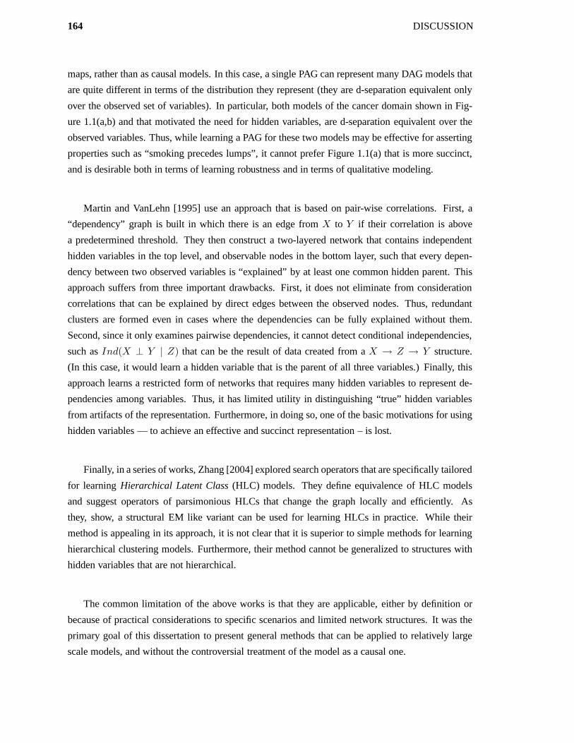
164 DISCUSSION
maps, rather than as causal models. In this case, a single PAG can represent many DAG models that
are quite different in terms of the distribution they represent (they are d-separation equivalent only
over the observed set of variables). In particular, both models of the cancer domain shown in Fig-
ure 1.1(a,b) and that motivated the need for hidden variables, are d-separation equivalent over the
observed variables. Thus, while learning a PAG for these two models may be effective for asserting
properties such as “smoking precedes lumps”, it cannot prefer Figure 1.1(a) that is more succinct,
and is desirable both in terms of learning robustness and in terms of qualitative modeling.
Martin and VanLehn [1995] use an approach that is based on pair-wise correlations. First, a
“dependency” graph is built in which there is an edge from X to Y if their correlation is above
a predetermined threshold. They then construct a two-layered network that contains independent
hidden variables in the top level, and observable nodes in the bottom layer, such that every depen-
dency between two observed variables is “explained” by at least one common hidden parent. This
approach suffers from three important drawbacks. First, it does not eliminate from consideration
correlations that can be explained by direct edges between the observed nodes. Thus, redundant
clusters are formed even in cases where the dependencies can be fully explained without them.
Second, since it only examines pairwise dependencies, it cannot detect conditional independencies,
such as Ind(X ⊥ Y | Z) that can be the result of data created from a X → Z → Y structure.
(In this case, it would learn a hidden variable that is the parent of all three variables.) Finally, this
approach learns a restricted form of networks that requires many hidden variables to represent de-
pendencies among variables. Thus, it has limited utility in distinguishing “true” hidden variables
from artifacts of the representation. Furthermore, in doing so, one of the basic motivations for using
hidden variables — to achieve an effective and succinct representation – is lost.
Finally, in a series of works, Zhang [2004] explored search operators that are specifically tailored
for learning Hierarchical Latent Class (HLC) models. They define equivalence of HLC models
and suggest operators of parsimonious HLCs that change the graph locally and efficiently. As
they, show, a structural EM like variant can be used for learning HLCs in practice. While their
method is appealing in its approach, it is not clear that it is superior to simple methods for learning
hierarchical clustering models. Furthermore, their method cannot be generalized to structures with
hidden variables that are not hierarchical.
The common limitation of the above works is that they are applicable, either by definition or
because of practical considerations to specific scenarios and limited network structures. It was the
primary goal of this dissertation to present general methods that can be applied to relatively large
scale models, and without the controversial treatment of the model as a causal one.

DISCUSSION 165
8.4 Future Prospects
The task of learning new hidden variables in probabilistic graphical model in general, and Bayesian
networks in particular, is a central and elusive challenge. This dissertation offers the first step
toward methods that treat this problem in a general context (e.g., Bayesian networks) without posing
restrictive constraints on the model.
The next natural step is to consider the application of the methods presented here for a wider
variety of models. This includes extensions to both undirected models (e.g., [Pearl, 1998]) and
Probabilistic Relational Models (PRMs) [Friedman et al., 1999a]. In the case of IB-EM, such ex-
tensions appear more subtle than for the other methods presented in this dissertation. Specifically,
in relational models, the instance identity takes on a different meaning: each object of each class
has an identity value and the data involves a single instance. This requires some adaptations to the
framework that change the semantics of the hidden variable. For undirected models we can use a
Chain Graph [Buntine, 1995] for Gout to encode the independencies of the target model and those
required by the IB-EM framework. This somewhat complicates computations but may lead to an
effective way of learning challenging undirected models using continuation.
— as a compression mechanism for the instance identity. The Information Bottleneck frame-
work, on which this method relies, is inherently directed in its construction, and need to be revisited
for undirected models.
Less clear, but of significant importance, is the extension to the hybrid models that allows both
discrete and continuous variables. Despite recent progress in learning methods for these networks
(e.g., [Lerner, 2002]), our understanding of how such a domain should be approached remains
limited. Adapting methods for learning new hidden variables in this scenario remains an important
challenge.
Several drawbacks of the different methods discussed in Section 8.2, may be overcome with
further investigations: Instead of the rigid structural signature currently used by FindHidden to
detect new hidden variables, we might be able to use soft confidence measures of edges and a
weighted measure for clique like structures. This will potentially result in an algorithm that is still
simple and easy to implement and that at the same time can be applied in the case of sparse data.
Another direction is to extend our Weight Annealing approach to utilize continuation. This will rid
the algorithm of an arbitrary cooling policy and will potentially results in comparable running times
to IB-EM. This can have important ramifications as Weight Annealing is already used successfully
in various learning problems [Friedman et al., 2001, Barash and Friedman, 2002].
Another important avenue of research is to improve our theoretical understanding of the methods
presented in the dissertation. The Weight Annealing toy problem presented in Chapter 3, hints of a
possibility of characterizing families of distributions for which the algorithm provably works; The
IB-EM framework offers the potential of adapting the theory to relational models; The Ideal Parent

166 DISCUSSION
approach can be extended to encompass a wider family of conditional probability distributions, such
as those that use multiplicative Gaussian noise.
Today, numerous challenging applications of graphical models use manually constructed hidden
variables to augment the expressiveness of the model. It is our belief that the methods presented
in this dissertation will pave the way to learning flexible probabilistic models with effective hidden
variables. It is our hope, that in this process, the hidden variables learned will not only increase
measurable qualitative performance, but also shed light on new and interesting domains.

Notation
X,Y,Z . . . random variables or their corresponding nodes in the network
X,Y,Z . . . sets of random variables or their corresponding nodes in the network
Val(X) the set of possible values of a discrete variable X
x, y, z . . . assignments to random variables
x,y, z . . . joint assignments to sets of random variables
(X ⊥ Y) independence of (sets of) random variables
Ind(X ⊥ Y | Z) conditional independence of (sets of) random variables
P (X) probability density of (sets of) random variables (P is used to denote P (X ))
P (X,Y,Z . . .) joint probability density of several (sets of) random variables
P (X | Y) conditional probability density of X given Y
B a Bayesian network
X the set of all variables in the network {X1, . . . ,XN}
G the graph structure of a network
θ the parameters of a network
θXi|Paiparameter of the CPD of Xi
θxi|paiparameter corresponding to the values xi and pai in the CPD of Xi
PaGi the parents variables of the variable Xi in G
ChGi the children variables of the variable Xi in G
FamGi the family of Xi in G (itself and its parents)
AdjGi the adjacent variables to Xi in G (its parent and children)
MBGi
the Markov blanket variables of Xi in G (its parent, children and their parents)
paGi an assignment to parents of Xi
N number of variables in the network
D the training data set
M number of instances in training set
S[xi,pai] the sufficient statistics count of xi and pai in D
H hidden variables
O observed variables
x[m] the value of x in the m’th sample
o[m] the m’th partially observed instance
L(θ,G : D) likelihood of the data given θ and G
`(θ,G : D) log-likelihood of the data given θ and G
LXi(θ,G : D) local likelihood of Xi’s family
`Xi(θ,G : D) local log-likelihood of Xi’s family
θ estimated parameters
αj hyper-parameters corresponding to the jth value in a multinomial distribution
αx
ji
hyper-parameters corresponding to the jth value of Xi
Score(G : D) score of G given D
167

Bibliography
J. Adachi and M. Hasegawa. Molphy version 2.3, programs for molecular phylogenetics based on
maximum likelihood. Technical report, The Institute of Statistical Mathematics, Tokyo, Japan,
1996.
H. Attias. Inferring parameters and structure of latent variable models by variational bayes. In
K. Laskey and H. Prade, editors, Proc. Fifteenth Conference on Uncertainty in Artificial Intelli-
gence (UAI ’99), pages 21–30, San Francisco, 1999. Morgan Kaufmann.
Y. Barash, G. Bejerano, and N. Friedman. A simple hyper-geometric approach for discovering
putative transcription factor binding sites. In O. Gascuel and B. M. E. Moret, editors, Algorithms
in Bioinformatics: Proceedings of the First International Workshop, number 2149 in LNCS,
pages 278–293. Springer, 2001.
Y. Barash and N. Friedman. Context-specific Bayesian clustering for gene expression data. Journal
of Computational Biology, 9:169–191, 2002.
R. Bareiss and B. Porter. Protos: An exemplar-based learning apprentice. Proc. 4th International
Workshop on Machine Learning, pages 12–23, 1987.
M. Behr, M. Wilson, W. Gill, H. Salamon, G. Schoolnik, S. Rand, and P. Small. Comparative
genomics of bcg vaccines by whole genome dna microarray. Science, 284:1520–1523, 1999.
I. Beinlich, G. Suermondt, R. Chavez, and G. Cooper. The ALARM monitoring system: A case
study with two probabilistic inference techniques for belief networks. In Proc. 2’nd European
Conference on AI and Medicine, volume 38, pages 247–256. Springer-Verlag, Berlin, 1989.
J. Binder, D. Koller, S. Russell, and K. Kanazawa. Adaptive probabilistic networks with hidden
variables. Machine Learning, 29:213–244, 1997.
C. M. Bishop. Neural Networks for Pattern Recognition. Oxford University Press, Oxford, United
Kingdom, 1995.
168

BIBLIOGRAPHY 169
C. Boutilier, N. Friedman, M. Goldszmidt, and D. Koller. Context-specific independence in
Bayesian networks. In E. Horvitz and F. Jensen, editors, Proc. Twelfth Conference on Uncertainty
in Artificial Intelligence (UAI ’96), pages 115–123, San Francisco, 1996. Morgan Kaufmann.
X. Boyen, N. Friedman, and D. Koller. Discovering the hidden structure of complex dynamic sys-
tems. In K. Laskey and H. Prade, editors, Proc. Fifteenth Conference on Uncertainty in Artificial
Intelligence (UAI ’99), pages 91–100, San Francisco, 1999. Morgan Kaufmann.
W. Buntine. Learning classification trees. In D. J. Hand, editor, Artificial Intelligence Frontiers in
Statistics, number III in AI and Statistics, pages 182–201. Chapman & Hall, London, 1993.
W. Buntine. Chain graphs for learning. In P. Besnard and S. Hanks, editors, Proc. Eleventh Con-
ference on Uncertainty in Artificial Intelligence (UAI ’95), pages 46–54, San Francisco, 1995.
Morgan Kaufmann.
K. Chang and R. Fung. Refinement and coarsening of bayesian networks. In P. P. Bonissone,
M. Henrion, L. N. Kanal, and J. F. Lemmer, editors, Proc. Sixth Annual Conference on Uncer-
tainty Artificial Intelligence (UAI ’90), pages 475–482, San Francisco, 1990. Morgan Kaufmann.
G. Chechik, A. Globerson, N. Tishby, and Y.Weiss. Gaussian information bottleneck. In S. Thrun,
L. K. Saul, and B. Scholkopf, editors, Advances in Neural Information Processing Systems 16,
Cambridge, Mass., 2003. MIT Press.
P. Cheeseman, J. Kelly, M. Self, J. Stutz, W. Taylor, and D. Freeman. Autoclass: a Bayesian
classification system. In Proc. Fifth International Workshop on Machine Learning, pages 54–64.
Morgan Kaufmann, San Francisco, 1988.
D. M. Chickering. A transformational characterization of equivalent Bayesian network structures.
In P. Besnard and S. Hanks, editors, Proc. Eleventh Conference on Uncertainty in Artificial Intel-
ligence (UAI ’95), pages 87–98, San Francisco, 1995. Morgan Kaufmann.
D. M. Chickering. Learning Bayesian networks is NP-complete. In D. Fisher and H. J. Lenz,
editors, Learning from Data: Artificial Intelligence and Statistics V, pages 121–130. Springer-
Verlag, New York, 1996a.
D. M. Chickering. Learning equivalence classes of Bayesian network structures. In E. Horvitz and
F. Jensen, editors, Proc. Twelfth Conference on Uncertainty in Artificial Intelligence (UAI ’96),
pages 150–157, San Francisco, 1996b. Morgan Kaufmann.
D. M. Chickering and D. Heckerman. Efficient approximations for the marginal likelihood of in-
complete data given a Bayesian network. In E. Horvitz and F. Jensen, editors, Proc. Twelfth
Conference on Uncertainty in Artificial Intelligence (UAI ’96), pages 158–168, San Francisco,
1996. Morgan Kaufmann.

170 BIBLIOGRAPHY
D. M. Chickering and D. Heckerman. Efficient approximations for the marginal likelihood of
Bayesian networks with hidden variables. Machine Learning, 29:181–212, 1997.
C. K. Chow and C. N. Liu. Approximating discrete probability distributions with dependence trees.
IEEE Trans. on Info. Theory, 14:462–467, 1968.
B. Codenotti, G. Manzini, L. Margara, and G. Resta. Perturbation: An efficient technique for the
solution of very large instances of the TSP. INFORMS Journal on Computing, 8(2):125–133,
1996.
G. F. Cooper. The computational complexity of probabilistic inference using Bayesian belief net-
works. Artificial Intelligence, 42:393–405, 1990.
G. F. Cooper and E. Herskovits. A Bayesian method for the induction of probabilistic networks
from data. Machine Learning, 9:309–347, 1992.
A. Corduneanu and T. Jaakkola. Continuation methods for mixing heterogeneous sources. In
A. Darwich and N. Friedman, editors, Proc. Eighteenth Conference on Uncertainty in Artificial
Intelligence (UAI ’02), pages 111–118, San Francisco, 2002. Morgan Kaufmann.
T. H. Cormen, C. E. Leiserson, and R. L. Rivest. Introduction to Algorithms. MIT Press, Cambridge,
Massachusetts, 1990.
T. M. Cover and J. A. Thomas. Elements of Information Theory. John Wiley & Sons, New York,
1991.
P. Dagum and M. Luby. An optimal approximation algorithm for Baysian inference. Artificial
Intelligence, 93(1–2):1–27, 1997.
T. Dean and K. Kanazawa. A model for reasoning about persistence and causation. Computational
Intelligence, 5:142–150, 1989.
R. Dechter. Bucket elimination: A unifying framework for probabilistic inference. In E. Horvitz
and F. Jensen, editors, Proc. Twelfth Conference on Uncertainty in Artificial Intelligence (UAI
’96), pages 211–219, San Francisco, 1996. Morgan Kaufmann.
M. H. DeGroot. Probability and Statistics. Addison Wesley, Reading, MA, 1989.
A. P. Dempster, N. M. Laird, and D. B. Rubin. Maximum likelihood from incomplete data via the
EM algorithm. Journal of the Royal Statistical Society, B 39:1–39, 1977.
F. J. Diez. Parameter adjustment in Bayes networks: The generalized noisy or-gate. In D. Hecker-
man and A. Mamdani, editors, Proc. Ninth Conference on Uncertainty in Artificial Intelligence
(UAI ’93), pages 99–105, San Francisco, 1993. Morgan Kaufmann.

BIBLIOGRAPHY 171
R. O. Duda and P. E. Hart. Pattern Classification and Scene Analysis. John Wiley & Sons, New
York, 1973.
R. Durbin, S. Eddy, A. Krogh, and G. Mitchison. Biological Sequence Analysis : Probabilistic
Models of Proteins and Nucleic Acids. Cambridge University Press, 1998.
B. Efron and R. J. Tibshirani. An Introduction to the Bootstrap. Chapman & Hall, London, 1993.
T. El-Hay and N Friedman. Incorporating expressive graphical models in variational approxima-
tions: Chain-graphs and hidden variables. In J.S. Breese and D. Koller, editors, Proc. Seventeenth
Conference on Uncertainty in Artificial Intelligence (UAI ’01), pages 136–143, San Francisco,
2001. Morgan Kaufmann.
G. Elidan and N. Friedman. Learning the dimensionality of hidden variables. In J.S. Breese and
D. Koller, editors, Proc. Seventeenth Conference on Uncertainty in Artificial Intelligence (UAI
’01), pages 144–151, San Francisco, 2001. Morgan Kaufmann.
G. Elidan and N. Friedman. The information bottleneck EM algorithm. In C. Meek and U. Kjærulff,
editors, Proc. Nineteenth Conference on Uncertainty in Artificial Intelligence (UAI ’03), pages
200–208, San Francisco, 2003. Morgan Kaufmann.
G. Elidan, N. Lotner, N. Friedman, and D. Koller. Discovering hidden variables: A structure-based
approach. In T. K. Leen, T. G. Dietterich, and V. Tresp, editors, Advances in Neural Information
Processing Systems 13, pages 479–485, Cambridge, Mass., 2001. MIT Press.
G. Elidan, M. Ninio, N. Friedman, and D. Schuurmans. Data perturbation for escaping local maxima
in learning. In Proc. National Conference on Artificial Intelligence (AAAI ’02), pages 132–139.
AAAI Press, Menlo Park, CA, 2002.
N. Friedman. Learning belief networks in the presence of missing values and hidden variables. In
D. Fisher, editor, Proc. Fourteenth International Conference on Machine Learning, pages 125–
133. Morgan Kaufmann, San Francisco, 1997.
N. Friedman. The Bayesian structural EM algorithm. In G. F. Cooper and S. Moral, editors,
Proc. Fourteenth Conference on Uncertainty in Artificial Intelligence (UAI ’98), pages 129–138,
San Francisco, 1998. Morgan Kaufmann.
N. Friedman, D. Geiger, and M. Goldszmidt. Bayesian network classifiers. Machine Learning, 29:
131–163, 1997.
N. Friedman, L. Getoor, D. Koller, and A. Pfeffer. Learning probabilistic relational models. In
Proc. Sixteenth International Joint Conference on Artificial Intelligence (IJCAI ’99), pages 1300–
1309. Morgan Kaufmann, San Francisco, 1999a.

172 BIBLIOGRAPHY
N. Friedman and M. Goldszmidt. Discretization of continuous attributes while learning Bayesian
networks. In L. Saitta, editor, Proc. Thirteenth International Conference on Machine Learning,
pages 157–165. Morgan Kaufmann, San Francisco, 1996a.
N. Friedman and M. Goldszmidt. Learning Bayesian networks with local structure. In E. Horvitz
and F. Jensen, editors, Proc. Twelfth Conference on Uncertainty in Artificial Intelligence (UAI
’96), pages 252–262, San Francisco, 1996b. Morgan Kaufmann.
N. Friedman, M. Goldszmidt, and A. Wyner. Data analysis with Bayesian networks: A bootstrap
approach. In K. Laskey and H. Prade, editors, Proc. Fifteenth Conference on Uncertainty in
Artificial Intelligence (UAI ’99), pages 196–205, San Francisco, 1999b. Morgan Kaufmann.
N. Friedman and D. Koller. Being Bayesian about Bayesian network structure: A Bayesian approach
to structure discovery in Bayesian networks. Machine Learning, 50:95–126, 2003.
N. Friedman, M. Linial, I. Nachman, and D. Pe’er. Using Bayesian networks to analyze expression
data. Computational Biology, 7:601–620, 2000.
N. Friedman, O. Mosenzon, N. Slonim, and N. Tishby. Multivariate information bottleneck. In
J.S. Breese and D. Koller, editors, Proc. Seventeenth Conference on Uncertainty in Artificial
Intelligence (UAI ’01), pages 152–161, San Francisco, 2001. Morgan Kaufmann.
N. Friedman, I. Nachman, and D. Pe’er. Learning bayesian network structure from massive datasets:
The “sparse candidate” algorithm. In K. Laskey and H. Prade, editors, Proc. Fifteenth Conference
on Uncertainty in Artificial Intelligence (UAI ’99), pages 206–215, San Francisco, 1999c. Morgan
Kaufmann.
N. Friedman, M. Ninio, I. Peer, and T. Pupko. A structural EM algorithm for phylogentic inference.
Journal of Computational Biology, 9:331–353, 2002.
A. P. Gasch, P. T. Spellman, C. M. Kao, O. Carmel-Harel, M. B. Eisen, G. Storz, D. Botstein,
and P. O. Brown. Genomic expression program in the response of yeast cells to environmental
changes. Molecular Biology of the Cell, 11:4241–4257, 2000.
D. Geiger and D. Heckerman. Learning gaussian networks. In R. Lopez de Mantaras and D. Poole,
editors, Proc. Tenth Conference on Uncertainty in Artificial Intelligence (UAI ’94), pages 235–
243, San Francisco, 1994. Morgan Kaufmann.
D. Geiger and D. Heckerman. Knowledge representation and inference in similarity networks and
Bayesian multinets. Artificial Intelligence, 82:45–74, 1996.

BIBLIOGRAPHY 173
D. Geiger, D. Heckerman, and C. Meek. Asymptotic model selection for directed networks with
hidden variables. In E. Horvitz and F. Jensen, editors, Proc. Twelfth Conference on Uncertainty
in Artificial Intelligence (UAI ’96), pages 283–290, San Francisco, 1996. Morgan Kaufmann.
D. Geiger and C. Meek. Graphical models and exponential families. In G. F. Cooper and S. Moral,
editors, Proc. Fourteenth Conference on Uncertainty in Artificial Intelligence (UAI ’98), pages
156–165, San Francisco, 1998. Morgan Kaufmann.
D. Geiger, T. S. Verma, and J. Pearl. Identifying independence in bayesian networks. Networks, 20:
507–534, 1990.
A. Gelman, J. B. Carlin, H. S. Stern, and D. B. Rubin. Bayesian Data Analysis. Chapman & Hall,
London, 1995.
W.R. Gilks, S. Richardson, and D.J. Spiegelhalter. Markov Chain Monte Carlo Methods in Practice.
CRC Press, 1996.
F. Glover and M. Laguna. Tabu search. In C. Reeves, editor, Modern Heuristic Techniques for
Combinatorial Problems, Oxford, England, 1993. Blackwell Scientific Publishing.
P.J. Green. Reversible jump Markov chain Monte Carlo computation and Bayesian model determi-
nation. Biometrika, 82:711–732, 1995.
D. Heckerman. A tutorial on learning with Bayesian networks. In M. I. Jordan, editor, Learning in
Graphical Models. Kluwer, Dordrecht, Netherlands, 1998.
D. Heckerman and D. Geiger. Learning Bayesian networks: a unification for discrete and Gaussian
domains. In P. Besnard and S. Hanks, editors, Proc. Eleventh Conference on Uncertainty in
Artificial Intelligence (UAI ’95), pages 274–284, San Francisco, 1995. Morgan Kaufmann.
D. Heckerman, D. Geiger, and D. M. Chickering. Learning Bayesian networks: The combination
of knowledge and statistical data. In R. Lopez de Mantaras and D. Poole, editors, Proc. Tenth
Conference on Uncertainty in Artificial Intelligence (UAI ’94), pages 293–301, San Francisco,
1994. Morgan Kaufmann.
D. Heckerman, D. Geiger, and D. M. Chickering. Learning Bayesian networks: The combination
of knowledge and statistical data. Machine Learning, 20:197–243, 1995a.
D. Heckerman, A. Mamdani, and M. P. Wellman. Real-world applications of Bayesian networks.
Communications of the ACM, 38, 1995b.
T. Hofmann and J. M. Buhmann. Pairwise data clustering by deterministic annealing. IEEE Trans-
actions on Pattern Analysis and Machine Intelligence, 19:1–14, 1997.

174 BIBLIOGRAPHY
T. R. Hughes, M. J. Marton, A. R. Jones, C. J. Roberts, R. Stoughton, C. D. Armour, H. A. Bennett,
E. Coffey, H. Dai, Y. D. He, M. J. Kidd, A. M. King, M. R. Meyer, D. Slade, P. Y. Lum, S. B.
Stepaniants, D. D. Shoemaker, D. Gachotte, K. Chakraburtty, J. Simon, M. Bard, and S. H. Friend.
Functional discovery via a compendium of expression profiles. Cell, 102(1):109–26, 2000.
E. T. Jaynes. Information theory and statistical mechanics. Physical Review, 106:620–630, 1957.
F. V. Jensen. An introduction to Bayesian Networks. University College London Press, London,
1996.
F. V. Jensen, S. L. Lauritzen, and K. G. Olesen. Bayesian updating in causal probabilistic networks
by local computations. Computational Statistics Quarterly, 5(4):269–282, 1990.
M. I. Jordan, Z. Ghahramani, T. Jaakkola, and L. K. Saul. An introduction to variational approx-
imations methods for graphical models. In M. I. Jordan, editor, Learning in Graphical Models.
Kluwer, Dordrecht, Netherlands, 1998.
S. Kirkpatrick, C. D. Gelatt, and M. P. Vecchi. Optimization by simulated annealing. Science, 220
(4598):671–680, 1983.
S. Kirpatrick, C.D. Gelatt, Jr., and M.P. Vecchi. Optimization by simulated annealing. Science, 220:
671–680, May 1994.
J. Kivinen and M. Warmuth. Exponentiated gradient versus gradient descent for linear predictors.
Information and Computation, 132:1–63, 1997.
T. Kocka and N. L. Zhang. Dimension correction for hierarchical latent class models. In A. Darwich
and N. Friedman, editors, Proc. Eighteenth Conference on Uncertainty in Artificial Intelligence
(UAI ’02), pages 267–274, San Francisco, 2002. Morgan Kaufmann.
S. Kullback and R. A. Leibler. On information and sufficiency. Annals of Mathematical Statistics,
22:76–86, 1951.
P. Laarhoven and E. Aarts. Simulated Annealing: Theory and Applications. John Wiley & Sons,
New York, 1987.
W. Lam and F. Bacchus. Learning Bayesian belief networks: An approach based on the MDL
principle. Computational Intelligence, 10:269–293, 1994.
K. Lang. Learning to filter netnews. In 12th International Conference on Machine Learning, pages
331–339. Morgan Kaufmann, San Francisco, California, 1995.
S. L. Lauritzen. The EM algorithm for graphical association models with missing data. Computa-
tional Statistics and Data Analysis, 19:191–201, 1995.

BIBLIOGRAPHY 175
S. L. Lauritzen and D. J. Spiegelhalter. Local computations with probabilities on graphical structures
and their application to expert systems. Journal of the Royal Statistical Society, B 50(2):157–224,
1988.
S. L. Lauritzen and N. Wermuth. Graphical models for associations between variables, some of
which are qualitative and some quantitative. Annals of Statistics, 17:31–57, 1989.
U. N. Lerner. Hybrid Bayesian Networks for Reasoning about Complex Systems. PhD thesis,
Dept. of Computer Science, Stanford University, 2002.
J. Martin and K. VanLehn. Discrete factor analysis: Learning hidden variables in Bayesian net-
works. Technical report, Department of Computer Science, University of Pittsburgh, 1995.
L. Mason, J. Baxter, P. Bartlett, and M. Frean. Functional gradient techniques for combining hy-
potheses. In Advances in Large Margin Classifiers. MIT Press, 2000.
P. McCullagh and J.A. Nelder. Generalized Linear Models. Chapman & Hall, London, 1989.
M. Meila and M. I. Jordan. Estimating dependency structure as a hidden variable. In M. I. Jordan,
M. J. Kearns, and S. A. Solla, editors, Advances in Neural Information Processing Systems 10,
pages 584–590, Cambridge, Mass., 1998. MIT Press.
N. Metropolis, A.W. Rosenbluth, M.N. Rosenbluth, A.H. Teller, and E. Teller. Equation of state
calculation by fast computing machines. Journal of Chemical Physics, 21:1087–1092, 1953.
R. Michalski and R. Chilausky. Learning by being told and learning from examples: An exper-
imental comparison of the two methods of knowledge acquisition in the context of developing
an expert system for soybean disease diagnosis. International Journal of Policy Analysis and
Information Systems, 4(2), 1980.
G. W. Milligan and M. C. Cooper. An examination of procedures for determining the number of
clusters in a data set. Psychometrika, 50:159–179, 1985.
K. Murphy and Y. Weiss. Loopy belief propagation for approximate inference: An empirical study.
In K. Laskey and H. Prade, editors, Proc. Fifteenth Conference on Uncertainty in Artificial Intel-
ligence (UAI ’99), pages 467–475, San Francisco, 1999. Morgan Kaufmann.
I. Nachman, A. Regev, and N. Friedman. Inferring quantitative models of regulatory networks from
expression data. Bioinformatics, 20(Suppl 1):S1248–1256, 2004.
R. M. Neal. Connectionist learning of belief networks. Artificial Intelligence, 56:71–113, 1992.
R. M. Neal. Probabilistic inference using Markov chain Monte Carlo methods. Technical Report
CRG-TR-93-1, Department of Computer Science, University of Toronto, 1993.

176 BIBLIOGRAPHY
R. M. Neal and G. E. Hinton. A new view of the EM algorithm that justifies incremental and other
variants. In M. I. Jordan, editor, Learning in Graphical Models. Kluwer, Dordrecht, Netherlands,
1998.
K. C. Nixon. The parsimony ratchet, a new method for rapid parsimony analysis. Cladistics, 15:
407–414, 1999.
J. Pearl. Probabilistic Reasoning in Intelligent Systems. Morgan Kaufmann, 1988.
J. Pearl. Graphs, causality, and structural equation models. Socioligical Methods and Research,
1998.
J. Pearl. Causality: Models, Reasoning, and Inference. Cambridge Univ. Press, 2000.
D. Pe’er, A. Regev, G. Elidan, and N. Friedman. Inferring subnetworks from perturbed expression
profiles. Bioinformatics, 17(Suppl 1):S215–24, 2001.
Fernando Pereira, Naftali Tishby, and Lillian Lee. Distributional clustering of English words. In
31st Annual Meeting of the ACL, pages 183–190, 1993.
Kim Leng Poh and Eric J. Horvitz. Reasoning about the value of decision-model refinement: Meth-
ods and application. In D. Heckerman and A. Mamdani, editors, Proc. Ninth Conference on
Uncertainty in Artificial Intelligence (UAI ’93), pages 174–182, San Francisco, 1993. Morgan
Kaufmann.
W. H. Price. Numerical Recipes in C. Cambridge University Press, Cambridge, 1992.
J. R. Quinlan. C4.5: Programs for Machine Learning. Morgan Kaufmann, San Francisco, Califor-
nia, 1993.
L. R. Rabiner. A tutorial on hidden Markov models and selected applications in speech recognition.
Proc. IEEE, 77(2):257–286, 1990.
K. Rose. Deterministic annealing for clustering, compression, classification, regression, and related
optimization problems. Proc. IEEE, 86:2210–2239, 1998.
D. R. Rubin. Inference and missing data. Biometrica, 63:581–592, 1976.
S. Russell and P. Norwig. Artificial Intelligence: A Modern Approach. Parentice Hall, 1995.
L. Saul, T. Jaakkola, and M. Jordan. Mean field theory for sigmoid belief networks. Journal of
Artificial Intelligence Research, 4:61–76, 1996.
R. E. Schapire and Y. Singer. Improved boosting algorithms using confidence-rated predictions.
Machine Learning, 37(3):297–336, 1999.

BIBLIOGRAPHY 177
D. Schuurmans, F. Southey, and R. Holte. The exponentiated subgradient algorithm for heuristic
Boolean programming. In Proc. Seventeenth International Joint Conference on Artificial Intelli-
gence (IJCAI ’01), pages 334–341, San Francisco, 2001. Morgan Kaufmann.
G. Schwarz. Estimating the dimension of a model. Annals of Statistics, 6:461–464, 1978.
E. Segal, Y. Barash, I. Simon, N. Friedman, and D. Koller. From promoter sequence to expression:
A probabilistic framekwork. In Gene Myers, Sridhar Hannenhalli, Sorin Istrail, Pavel Pevzner,
and Michael Waterman, editors, Proceedings of the Sixth Annual International Conference on
Computational Biology (RECOMB ’02), pages 263–272. ACM Press, New York, 2002.
R. Settimi and J. Q. Smith. On the geometry of bayesian graphical models with hidden variables.
In G. F. Cooper and S. Moral, editors, Proc. Fourteenth Conference on Uncertainty in Artificial
Intelligence (UAI ’98), pages 472–479, San Francisco, 1998. Morgan Kaufmann.
M.A. Shwe, B. Middleton, D.E. Heckerman, M. Henrion, E.J. Horvitz, H.P. Lehmann, and G.F.
Cooper. Probabilistic diagnosis using a reformulation of the INTERNIST-1/QMR knowledge
base. I. The probabilistic model and inference algorithms. Methods of Information in Medicine,
30:241–55, 1991.
I. Simon, J. Barnett, N. Hannett, C.T. Harbison, N.J. Rinaldi, T.L. Volkert, J.J. Wyrick, J. Zeitlinger,
D.K. Gifford, T.S. Jaakkola, and R.A. Young. Serial regulation of transcriptional regulators in
the yeast cell cycle. Cell, 106:697–708, 2001.
N. Slonim, N.Friedman, and T.Tishby. Agglomerative multivariate information bottleneck. In T. G.
Dietterich, S. Becker, and Z. Ghahramani, editors, Advances in Neural Information Processing
Systems 14, pages 929–936, Cambridge, Mass., 2002. MIT Press.
N. Slonim and N. Tishby. Agglomerative information bottleneck. In S. A. Solla, T. K. Leen,
and K. Muller, editors, Advances in Neural Information Processing Systems 12, pages 617–623,
Cambridge, Mass., 2000. MIT Press.
N. Slonim and N. Tishby. Data clustering by markovian relaxation and the information bottleneck
method. In T. K. Leen, T. G. Dietterich, and V. Tresp, editors, Advances in Neural Information
Processing Systems 13, pages 640–646, Cambridge, Mass., 2001. MIT Press.
N. Slonim and Y. Weiss. Maximum likelihood and the information bottleneck. In S. Becker,
S. Thrun, and K. Obermayer, editors, Advances in Neural Information Processing Systems 15,
pages 351–358, Cambridge, Mass., 2002. MIT Press.
N. A. Smith and J. Eisner. Annealing techniques for unsupervised statistical language learning. In
Proc. 42nd Annual Meeting of the Association for Computational Linguistics, 2004.

178 BIBLIOGRAPHY
P. T. Spellman, G. Sherlock, M. Q. Zhang, V. R. Iyer, K. Anders, M. B. Eisen, P. O. Brown, D. Bot-
stein, and B. Futcher. Comprehensive identification of cell cycle-regulated genes of the yeast
saccharomyces cerevisiae by microarray hybridization. Molecular Biology of the Cell, 9(12):
3273–97, 1998.
D. J. Spiegelhalter and S. L. Lauritzen. Sequential updating of conditional probabilities on directed
graphical structures. Networks, 20:579–605, 1990.
P. Spirtes, C. Glymour, and R. Scheines. Causation, Prediction and Search. Number 81 in Lecture
Notes in Statistics. Springer-Verlag, New York, 1993.
P. Spirtes, C. Meek, and T. Richardson. Causal inference in the presence of latent variables and
selection bias. In P. Besnard and S. Hanks, editors, Proc. Eleventh Conference on Uncertainty in
Artificial Intelligence (UAI ’95), pages 499–506, San Francisco, 1995. Morgan Kaufmann.
A. Stolcke and S. Omohundro. Hidden Markov Model induction by bayesian model merging. In
Stephen Jose Hanson, Jack D. Cowan, and C. Lee Giles, editors, Advances in Neural Information
Processing Systems, volume 5, pages 11–18. Morgan Kaufmann, San Mateo, CA, 1993.
A. Stolcke and S. Omohundro. Inducing probabilistic grammars by bayesian model merging. In
Proc. Second International Conference on Grammatical Inference, pages 106–118, New York,
1994. Springer-Verlag.
M. Szummer and T. Jaakkola. Information regularization with partially labeled data. In S. Becker,
S. Thrun, and K. Obermayer, editors, Advances in Neural Information Processing Systems 15,
pages 640–646, Cambridge, Mass., 2002. MIT Press.
B. Thiesson, C. Meek, D. M. Chickering, and D. Heckerman. Learning mixtures of Bayesian
networks. In G. F. Cooper and S. Moral, editors, Proc. Fourteenth Conference on Uncertainty in
Artificial Intelligence (UAI ’98), pages 504–513, San Francisco, 1998. Morgan Kaufmann.
N. Tishby, F. Pereira, and W. Bialek. The information bottleneck method. In B. Hajek and R. S.
Sreenivas, editors, Proc. 37th Allerton Conference on Communication, Control and Computation,
pages 368–377. University of Illinois, 1999.
R. Parr U. Lerner and D. Koller. Bayesian fault detection and diagnosis in dynamic systems. In
Proc. of the Seventeenth National Conference on Artificial Intelligence (AAAI), pages 531–537,
2000.
N. Ueda and R. Nakano. Deterministic annealing EM algorithm. Neural Networks, 11(2):271–282,
1998.
BIBLIOGRAPHY 179
S. Waterhouse, D. Mackay, and T. Robinson. Bayesian methods for mixtures of experts. In D. S.
Touretzky, M. Mozer, and M. E. Hasselmo, editors, Advances in Neural Information Processing
Systems 8, pages 351–357, Cambridge, Massachusetts, 1996. MIT Press.
L. T. Watson. Theory of globally convergent probability-one homotopies for non-linear program-
ming. Technical Report TR-00-04, Department of Computer Science, Virginia Tech, 2000.
M. P. Wellman and C.-L. Liu. State-space abstraction for anytime evaluation of probabilistic net-
works. In R. Lopez de Mantaras and D. Poole, editors, Proc. Tenth Conference on Uncertainty in
Artificial Intelligence (UAI ’94), pages 567 – 574, San Francisco, 1994. Morgan Kaufmann.
M. Whiley and D. M. Titterington. Applying the deterministic annealing expectation maximization
algorithm to Naive Bayes networks. Technical Report 02-5, Department of Statistics, University
of Glasgow, 2002.
J. Wilkinson. The algebric eigenvalue problem. Claderon Press, Oxford, 1965.
S. Wright. Correlation and causation. Journal of Agricultural Research, 20:557–585, 1921.
N.L. Zhang. Hierarchical latent class models for cluster analysis. Journal of Machine Learning
Research, 5:697–723, 2004.