learning image representations tied to egomotion...
TRANSCRIPT
IJCV Special Issue (Best Papers from ICCV 2015) manuscript No.(will be inserted by the editor)
Learning image representations tied to egomotionfrom unlabeled video
Dinesh Jayaraman · Kristen Grauman
Received: 16 June 2016 / Accepted: Feb 10, 2017
Abstract Understanding how images of objects and scenes behave in responseto specific egomotions is a crucial aspect of proper visual development, yet ex-isting visual learning methods are conspicuously disconnected from the phys-ical source of their images. We propose a new “embodied” visual learningparadigm, exploiting proprioceptive motor signals to train visual representa-tions from egocentric video with no manual supervision. Specifically, we enforcethat our learned features exhibit equivariance i.e., they respond predictablyto transformations associated with distinct egomotions. With three datasets,we show that our unsupervised feature learning approach significantly outper-forms previous approaches on visual recognition and next-best-view predictiontasks. In the most challenging test, we show that features learned from videocaptured on an autonomous driving platform improve large-scale scene recog-nition in static images from a disjoint domain.
1 Introduction
How is visual learning shaped by egomotion? In their famous “kitten carousel”experiment, psychologists Held and Hein examined this question in 1963 [18].To analyze the role of self-produced movement in perceptual development, theydesigned a carousel-like apparatus in which two kittens could be harnessed.For eight weeks after birth, the kittens were kept in a dark environment, ex-cept for one hour a day on the carousel. One kitten, the “active” kitten, couldmove freely of its own volition while attached. The other kitten, the “passive”
D. JayaramanThe University of Texas at AustinE-mail: [email protected]
K. GraumanThe University of Texas at AustinE-mail: [email protected]
2 Dinesh Jayaraman, Kristen Grauman
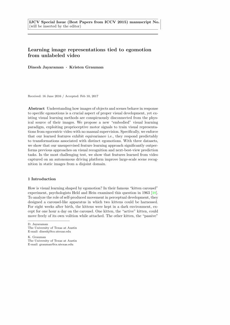
Fig. 1 Schematic figure from [18] showing the apparatus for the kitten carousel study. Theactive kitten ’A’ was free to move itself in both directions around the three axes of rotationa-a, b-b and c-c, while pulling the passive kitten ’P’ through the equivalent movementsaround a-a, b-b and d-d by means of the mechanical linkages in the carousel setup.
kitten, was carried along in a basket and could not control his own movement;rather, he was forced to move in exactly the same way as the active kitten.Fig 1 shows a schematic of the apparatus. Thus, both kittens had identical vi-sual experiences. However, while the active kitten simultaneously experiencedsignals about his own motor actions, the passive kitten was simply along forthe ride. It saw what the active kitten saw, but it could not simultaneouslylearn from self-generated motion signals.
The outcome of the experiment is remarkable. After eight weeks, the activekitten’s visual perception was indistinguishable from kittens raised normally,whereas the passive kitten suffered fundamental problems. The implication isclear: proper perceptual development requires leveraging self-generated move-ment in concert with visual feedback. Specifically, the active kitten had twoadvantages over the passive kitten: (i) it had proprioceptive knowledge of thespecific motions of its body that were causing the visual responses it was ob-serving, and (ii) it had the ability to select those motions in the first place.The results of this experiment establish that these advantages are critical tothe development of visual perception.
We contend that today’s visual recognition algorithms are crippled muchlike the passive kitten. The culprit: learning from “bags of images”. Ever sincestatistical learning methods emerged as the dominant paradigm in the recog-nition literature, the norm has been to treat images as i.i.d. draws from an un-derlying distribution. Whether learning object categories, scene classes, bodyposes, or features themselves, the idea is to discover patterns within a collec-tion of snapshots, blind to their physical source. So is the answer to learn fromvideo? Only partially. As we can see from the kitten carousel experiment, or
Learning image representations tied to egomotion from unlabeled video 3
in general from observing biological perceptual systems, vision develops in thecontext of acting and moving in the world. Without leveraging the accompa-nying motor signals initiated by the observer, learning from video data doesnot escape the passive kitten’s predicament.
Inspired by this concept, we propose to treat visual learning as an embodiedprocess, where the visual experience is inextricably linked to the motor activitybehind it.1 In particular, our goal is to learn representations that exploit theparallel signals of egomotion and pixel appearance. As we will explain below,we hypothesize that downstream processing will benefit from access to suchrepresentations.
To this end, we attempt to learn the connection between how an observermoves, and how its visual surroundings change. We do this by exploiting motorsignals accompanying unlabeled egocentric video, of the sort that one couldobtain from a wearable platform like Google Glass, a self-driving car, or evena mobile phone camera.
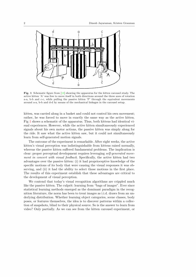
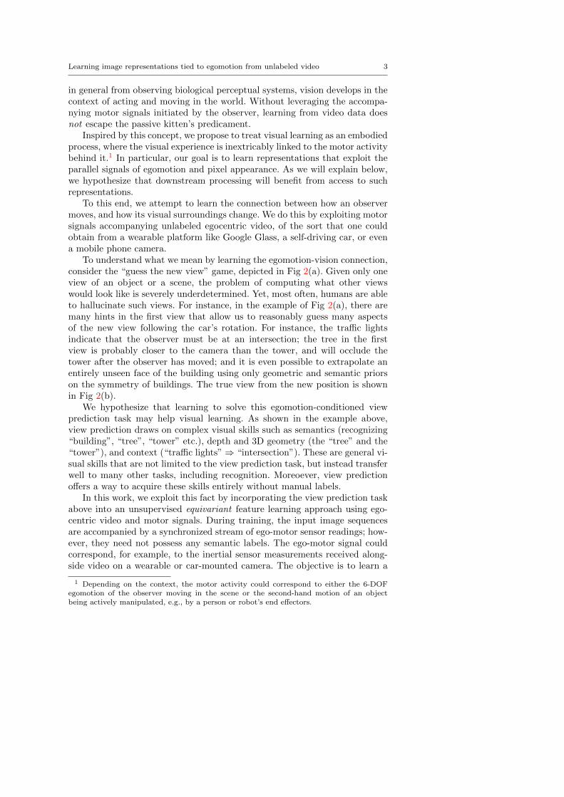
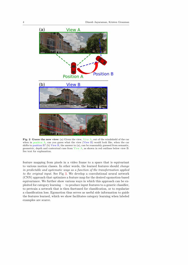
To understand what we mean by learning the egomotion-vision connection,consider the “guess the new view” game, depicted in Fig 2(a). Given only oneview of an object or a scene, the problem of computing what other viewswould look like is severely underdetermined. Yet, most often, humans are ableto hallucinate such views. For instance, in the example of Fig 2(a), there aremany hints in the first view that allow us to reasonably guess many aspectsof the new view following the car’s rotation. For instance, the traffic lightsindicate that the observer must be at an intersection; the tree in the firstview is probably closer to the camera than the tower, and will occlude thetower after the observer has moved; and it is even possible to extrapolate anentirely unseen face of the building using only geometric and semantic priorson the symmetry of buildings. The true view from the new position is shownin Fig 2(b).
We hypothesize that learning to solve this egomotion-conditioned viewprediction task may help visual learning. As shown in the example above,view prediction draws on complex visual skills such as semantics (recognizing“building”, “tree”, “tower” etc.), depth and 3D geometry (the “tree” and the“tower”), and context (“traffic lights” ⇒ “intersection”). These are general vi-sual skills that are not limited to the view prediction task, but instead transferwell to many other tasks, including recognition. Moreoever, view predictionoffers a way to acquire these skills entirely without manual labels.
In this work, we exploit this fact by incorporating the view prediction taskabove into an unsupervised equivariant feature learning approach using ego-centric video and motor signals. During training, the input image sequencesare accompanied by a synchronized stream of ego-motor sensor readings; how-ever, they need not possess any semantic labels. The ego-motor signal couldcorrespond, for example, to the inertial sensor measurements received along-side video on a wearable or car-mounted camera. The objective is to learn a
1 Depending on the context, the motor activity could correspond to either the 6-DOFegomotion of the observer moving in the scene or the second-hand motion of an objectbeing actively manipulated, e.g., by a person or robot’s end effectors.
4 Dinesh Jayaraman, Kristen Grauman
View A
Position APosition B
View B
(a)
(b)
Fig. 2 Guess the new view: (a) Given the view, View A, out of the windshield of the carwhen in position A, can you guess what the view (View B) would look like, when the carshifts to position B? (b) View B, the answer to (a), can be reasonably guessed from semantic,geometric, depth and contextual cues from View A, as shown in red outlines below view B.See text for explanation.
feature mapping from pixels in a video frame to a space that is equivariantto various motion classes. In other words, the learned features should changein predictable and systematic ways as a function of the transformation appliedto the original input. See Fig 3. We develop a convolutional neural network(CNN) approach that optimizes a feature map for the desired egomotion-basedequivariance. We further show various ways in which this approach can be ex-ploited for category learning — to produce input features to a generic classifier,to pretrain a network that is then finetuned for classification, or to regularizea classification loss. Egomotion thus serves as useful side information to guidethe features learned, which we show facilitates category learning when labeledexamples are scarce.
Learning image representations tied to egomotion from unlabeled video 5
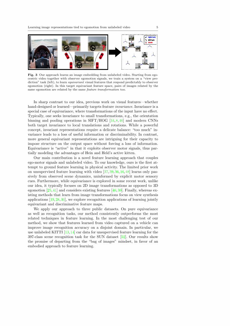
Fig. 3 Our approach learns an image embedding from unlabeled video. Starting from ego-centric video together with observer egomotion signals, we train a system on a “view pre-diction” task (left), to learn equivariant visual features that respond predictably to observeregomotion (right). In this target equivariant feature space, pairs of images related by thesame egomotion are related by the same feature transformation too.
In sharp contrast to our idea, previous work on visual features—whetherhand-designed or learned—primarily targets feature invariance. Invariance is aspecial case of equivariance, where transformations of the input have no effect.Typically, one seeks invariance to small transformations, e.g., the orientationbinning and pooling operations in SIFT/HOG [34,8,46] and modern CNNsboth target invariance to local translations and rotations. While a powerfulconcept, invariant representations require a delicate balance: “too much” in-variance leads to a loss of useful information or discriminability. In contrast,more general equivariant representations are intriguing for their capacity toimpose structure on the output space without forcing a loss of information.Equivariance is “active” in that it exploits observer motor signals, thus par-tially modeling the advantages of Hein and Held’s active kitten.
Our main contribution is a novel feature learning approach that couplesego-motor signals and unlabeled video. To our knowledge, ours is the first at-tempt to ground feature learning in physical activity. The limited prior workon unsupervised feature learning with video [37,39,36,16,48] learns only pas-sively from observed scene dynamics, uninformed by explicit motor sensorycues. Furthermore, while equivariance is explored in some recent work, unlikeour idea, it typically focuses on 2D image transformations as opposed to 3Degomotion [25,41] and considers existing features [46,30]. Finally, whereas ex-isting methods that learn from image transformations focus on view synthesisapplications [19,28,36], we explore recognition applications of learning jointlyequivariant and discriminative feature maps.
We apply our approach to three public datasets. On pure equivarianceas well as recognition tasks, our method consistently outperforms the mostrelated techniques in feature learning. In the most challenging test of ourmethod, we show that features learned from video captured on a vehicle canimprove image recognition accuracy on a disjoint domain. In particular, weuse unlabeled KITTI [13,14] car data for unsupervised feature learning for the397-class scene recognition task for the SUN dataset [52]. Our results showthe promise of departing from the “bag of images” mindset, in favor of anembodied approach to feature learning.
6 Dinesh Jayaraman, Kristen Grauman
2 Related work
Invariant features Invariance is a special case of equivariance, wherein a trans-formed output remains identical to its input. Invariance is known to be valu-able for visual representations. Descriptors like SIFT [34], HOG [8], and as-pects of CNNs like pooling and convolution, are hand-designed for invarianceto small shifts and rotations. Feature learning work aims to learn invariancesfrom data [42,43,47,44,11]. Strategies include augmenting training data byperturbing image instances with label-preserving transformations [43,47,11],and inserting linear transformation operators into the feature learning algo-rithm [44].
Most relevant to our work are feature learning methods based on temporalcoherence and “slow feature analysis” [50,17,37]. The idea is to require thatlearned features vary slowly over continuous video, since visual stimuli canonly gradually change between adjacent frames. Temporal coherence has beenexplored for unsupervised feature learning with CNNs [37,55,16,5,33,48,12],with applications to dimensionality reduction [17], object recognition [37,55],and metric learning [16]. Temporal coherence of inferred body poses in unla-beled video is exploited for invariant recognition in [6]. These methods exploitvideo as a source of free supervision to achieve invariance, analogous to the im-age perturbations idea above. In contrast, our method exploits video coupledwith ego-motor signals to achieve the more general property of equivariance.
Equivariant representations Equivariant features can also be hand-designedor learned. For example, equivariant or “co-variant” operators are designedto detect repeatable interest points [46]. Recent work explores ways to learndescriptors with in-plane translation/rotation equivariance [25,41]. While thelatter does perform feature learning, its equivariance properties are crafted forspecific 2D image transformations. In contrast, we target more complex equiv-ariances arising from natural observer motions (3D egomotion) that cannoteasily be crafted, and our method learns them from data.
Methods to learn representations with disentangled latent factors [19,28]aim to sort properties like pose and illumination into distinct portions of thefeature space. For example, the transforming auto-encoder learns to explicitlyrepresent instantiation parameters of object parts in equivariant hidden layerunits [19]. Such methods target equivariance in the limited sense of inferringpose parameters, which are appended to a conventional feature space designedto be invariant. In contrast, our formulation encourages equivariance over thecomplete feature space; we show the impact as an unsupervised regularizerwhen training a recognition model with limited training data.
It has been shown to be possible to predict poses of objects using de-scriptors learned for classification tasks [45]. The work of [30] quantifies theinvariance/equivariance of various standard representations, including CNNfeatures, in terms of their responses to specified in-plane 2D image transforma-tions (affine warps, flips of the image). We adopt the definition of equivarianceused in that work, but our goal is entirely different. While these works demon-
Learning image representations tied to egomotion from unlabeled video 7
strate and/or quantify the equivariance of existing descriptors, our approachfocuses on learning a feature space that is equivariant.
Learning transformations Other methods train with pairs of transformed im-ages and infer an implicit representation for the transformation itself. In [35],bilinear models with multiplicative interactions are used to learn content-independent “motion features” that encode only the transformation betweenimage pairs. One such model, the “gated autoencoder” is extended to per-form sequence prediction for video in [36]. Recurrent neural networks com-bined with a grammar model of scene dynamics can also predict future framesin video [39]. Whereas these methods learn a representation for image pairs(or tuples) related by some transformation, we learn a representation for in-dividual images in which the behavior under transformations is predictable.Furthermore, whereas these prior methods abstract away the image content,our method preserves it, making our features relevant for recognition.
Egocentric vision There is renewed interest in egocentric computer visionmethods, though none perform feature learning using motor signals and pix-els in concert as we propose. Recent methods use egomotion cues to separateforeground and background [40,53] or infer the first-person gaze [54,32]. Whilemost work relies solely on apparent image motion, the method of [53] exploitsa robot’s motor signals to detect moving objects and [38] uses reinforcementlearning to form robot movement policies by exploiting correlations betweenmotor commands and observed motion cues.
Vision from/for motion Very recently, concurrently with our work, and inde-pendent of it, a growing body of work [7,26,49,2,3,31] studies the interactionbetween high-level visual tasks and agent actions or motions. Among these, [31,26,49,3] focus on end-to-end learning of visual representations targeting ac-tion tasks such as driving. Some work also studies the theoretical propertiesof visual representations that vary linearly with observer motion [7], a formof equivariance, or learns a visual representation space in which control taskssimplify to linear operations [49]. Of all these recent works, the closest toours is [2], which uses a different approach to ours to learn visual represen-tations from video with associated egomotion sensor streams. Rather thanlearn to predict a new view given the starting view and the egomotion aswe do, their method learns to predict the egomotion, given the original andfinal views. Conceptually, while our approach explicitly targets a desired prop-erty, egomotion-equivariance, in the learned feature space, the method of [2]treats their egomotion-regression task as a generic proxy task for representa-tion learning. We compare against their method in our experiments in Sec 4.
Finally, this manuscript builds upon our previous work published in ICCV2015 [21]. Specifically, we make the following additional contributions in thiswork: (i) we conceptually extend our equivariant feature learning formulationto handle non-discrete motions and more general definitions of equivariance
8 Dinesh Jayaraman, Kristen Grauman
(Sec 3.4), (ii) we empirically verify that our method scales up to much largerimages than in previous tests (Sec 4.4), (iii) we study the impact of the equiv-ariance objective on multiple layers of features in a deep neural network ar-chitecture (Sec 4.4), (iv) we show that features trained purely for equivariancein our formulation, entirely without manual supervision, may be used as in-puts to a generic classifier for recognition tasks (Sec 4.4), (v) we empiricallyverify that the network weights corresponding to such purely unsupervisedequivariant features may be finetuned for recognition tasks (Sec 4.4), (vi) weperform new experiments allowing the direct comparison of features learned ina neural network classifier with unsupervised egomotion-equivariance regular-ization, and features trained purely for egomotion-equivariance (Sec 4.5) (vii)we present alternative intuitions supporting our equivariance formulation interms of new view prediction (Sec 1), (viii) we compare our approach againsta new baseline, lsm [2], and (ix) we significantly extend all sections of the pa-per, including our descriptions of the method, its motivations and experiments,with additional illustrations for the sake of clarity and completeness.
3 Approach
Our goal is to learn an image representation that is equivariant with respectto egomotion transformations. Let xi ∈ X be an image in the original pixelspace, and let yi ∈ Y be its associated ego-pose representation. The ego-posecaptures the available motor signals, and could take a variety of forms. Forexample, Y may encode the complete observer camera pose (its position in 3Dspace, pitch, yaw, roll), some subset of those parameters, or any reading froma motor sensor paired with the camera.
As input to our learning algorithm, we have a training set U ofNu unlabeledimage pairs and their associated ego-poses, U = {〈(xi,xj), (yi,yj)〉}Nu
(i,j)=1}.The image pairs originate from video sequences, though they need not beadjacent frames in time. The set may contain pairs from multiple videos andcameras. Note that this training data does not have any semantic labels (objectcategories, etc.); they are “labeled” only in terms of the ego-motor sensorreadings. Since our method relies on freely available motion sensor readingsassociated with video streams (e.g., from Google glass, self-driving cars, oreven hand-held mobile devices), rather than on expensive manually suppliedlabels, it is effectively unsupervised.2
In the following, we first explain how to translate ego-pose informationinto pairwise “motion pattern” annotations (Sec 3.1). Then, Sec 3.2 definesthe precise nature of the equivariance we seek, and Sec 3.3 defines our learning
2 One could attempt to apply our idea using camera poses inferred from the video itself(i.e., with structure from motion). However, there are conceptual and practical advantagesto relying instead on external sensor data capturing egomotion. First, the sensor data, whenavailable, is much more efficient to obtain and can be more reliable. Second, the use ofan external sensor parallels the desired effect of the agent learning from its proprioceptionmotor signals, as opposed to bootstrapping the visual learning process from a previouslydefined visual odometry module based on the same visual input stream.
Learning image representations tied to egomotion from unlabeled video 9
objective. We define a variant of our approach using non-discrete egomotionpatterns and non-linear equivariance maps in Sec 3.4. Then, in Sec 3.5, weshow how a feedforward neural network architecture may be trained to pro-duce the desired equivariant feature space. Finally, Sec 3.6 shows how ourequivariant feature learning scheme may be used to enhance recognition withlimited training data.
3.1 Mining discrete egomotion patterns
First we want to organize training sample pairs into a discrete set of egomotionpatterns G. For instance, one egomotion pattern might correspond to “tiltdownwards by approximately 20◦”. As we will see in Sec 3.3, translating rawegomotion signals into a few discrete motion patterns helps to simplify thedesign of our system. While one could collect new data explicitly controllingfor the patterns (e.g., with a turntable and camera rig), we prefer a data-drivenapproach that can leverage video and ego-pose data collected “in the wild”.
To this end, we discover clusters among pose difference vectors yi − yj forpairs (i, j) of temporally close frames from video (typically less than 1 secondapart; see Sec 4.1 for details). For simplicity we apply k-means to find Gclusters, though other methods are possible. Let pij ∈ P = {1, . . . , G} denotethe motion pattern ID, i.e., the cluster to which (yi,yj) belongs. We can nowreplace the ego-pose vectors in U with motion pattern IDs: 〈(xi,xj), pij〉. 3
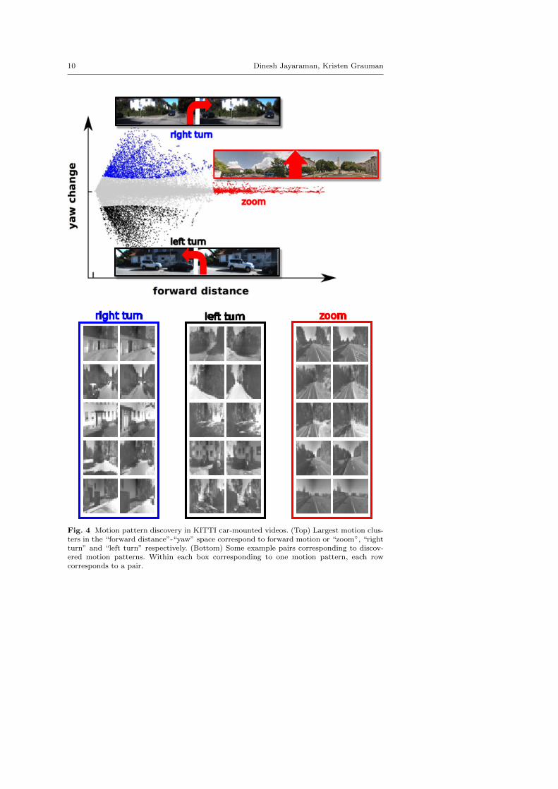
Fig 4 illustrates motion pattern discovery on frame pairs from the KITTIdataset [13,14] videos, which are captured from a moving car. Here Y consistsof the position and yaw angle of the camera. So, we are clustering a 2D spaceconsisting of forward distance and change in yaw. As shown in the bottompanel, the largest clusters correspond to the car’s three primary egomotions:turning left, turning right, and going forward.
In Sec 3.4 we discuss a variant of our approach that operates with non-discrete motion patterns.
3.2 Definition of egomotion equivariance
Given U , we wish to learn a feature mapping function zθ(.) : X → RD param-eterized by θ that maps a single image to a D-dimensional vector space thatis equivariant to egomotion.
To define equivariance, it is convenient to start with the notion of fea-ture invariance, which is the standard property that visual representationsfor recognition are designed to exhibit. Invariant features are unresponsive tocertain classes of so-called “nuisance transformations” such as observer ego-motions, pose change, or illumination change. For images xi and xj with
3 For movement with d degrees of freedom, setting G ≈ d should suffice (cf. Sec 3.2).Sec 3.3 discusses tradeoffs involved in selecting G. We chose a small value for G for efficiencyand did not vary it in experiments.
10 Dinesh Jayaraman, Kristen Grauman
right turn zoomleft turn
Fig. 4 Motion pattern discovery in KITTI car-mounted videos. (Top) Largest motion clus-ters in the “forward distance”-“yaw” space correspond to forward motion or “zoom”, “rightturn” and “left turn” respectively. (Bottom) Some example pairs corresponding to discov-ered motion patterns. Within each box corresponding to one motion pattern, each rowcorresponds to a pair.
Learning image representations tied to egomotion from unlabeled video 11
associated ego-poses yi and yj respectively, an egomotion-invariant featuremapping function zθ satisfies:
zθ(xj) ≈ zθ(xi). (1)
Recall that this is the form representation sought by many existing featurelearning methods, including those that learn representations from video [37,55,16,5,33,48,12].
Rather than being unresponsive as above, equivariant functions are pre-dictably responsive to transformations, i.e., an egomotion-equivariant functionzθ must respond systematically and predictably to egomotions:
zθ(xj) ≈ f(zθ(xi),yi,yj), (2)
for some simple function f ∈ F , where again yi denotes the ego-pose meta-data associated with video frame xi. Note that f must be simple; as the spaceof allowed functions F grows larger, the requirement in Eq (2) above is satisfiedby more feature mapping functions zθ. In other words, as F grows large, theequivariance constraint on zθ grows weak.
We will first consider equivariance for linear functions f(.), following [30].Later, in Sec 3.4, we will show how to extend this to the non-linear case. In thelinear case, zθ is said to be equivariant with respect to some transformation gif there exists a D ×D matrix4 Mg such that:
∀x ∈ X : zθ(gx) ≈ Mgzθ(x). (3)
Such an Mg is called the “equivariance map” of g on the feature space zθ(.).It represents the affine transformation in the feature space that correspondsto transformation g in the pixel space. For example, suppose a motion patterng corresponds to a yaw turn of 20◦, and x and gx are the images observedbefore and after the turn, respectively. Equivariance demands that there issome matrix Mg that maps the pre-turn image to the post-turn image, oncethose images are expressed in the feature space zθ. Hence, zθ “organizes”the feature space in such a way that movement in a particular direction in thefeature space (here, as computed by matrix-vector multiplication withMg) hasa predictable outcome. The linear case, as also studied in [30], ensures thatthe structure of the mapping has a simple form — the space F of possibleequivariance maps is suitably restricted so that the equivariance constraintis significant, as discussed above. It is also convenient for learning since Mg
can be encoded as a fully connected layer in a neural network. In Sec 4, weexperiment with both linear and simple non-linear equivariance maps.
3.2.1 Equivariance in dynamic 3D scenes
While prior work [25,41] focuses on equivariance where g is a 2D image warp,we explore the case where g ∈ P is an egomotion pattern (cf. Sec 3.1) reflecting
4 bias dimension assumed to be included in D for notational simplicity
12 Dinesh Jayaraman, Kristen Grauman
the observer’s 3D movement in the world. In theory, appearance changes of animage in response to an observer’s egomotion are not determined completelyby the egomotion alone. They also depend on the depth map of the sceneand the motion of dynamic objects in the scene. One could easily augmenteither the frames xi or the ego-pose yi with depth maps, when available.Non-observer motion appears more difficult, especially in the face of changingocclusions and newly appearing objects. Even accounting for everything, afuture frame may never be fully predictable purely from egomotion alone,due to changing occlusions/ newly visible elements in the scene. However, ourexperiments indicate we can learn effective representations even with dynamicobjects and changing occlusions. In our implementation, we train with pairsrelatively close in time, so as to avoid some of these pitfalls.
3.2.2 Equivariance to composite motions
While during training we target equivariance for the discrete set of G egomo-tions, if we use linear equivariance maps as above, the learned feature spacewill not be limited to preserving equivariance for pairs originating from thesame egomotions. This is because the linear equivariance maps are compos-able. If we are operating in a space where every egomotion can be composedas a sequence of “atomic” motions, equivariance to those atomic motions issufficient to guarantee equivariance to all motions.
To see this, suppose that the maps for “turn head right by 10◦” (egomotionpattern r) and “turn head up by 10◦” (egomotion pattern u) are respectivelyMr and Mu, i.e, z(rx) = Mrz(x) and z(ux) = Muz(x) for all x ∈ X . Now fora novel diagonal motion d that can be composed from these atomic motionsas d = r ◦ u (“turn head up by 10◦, then right by 10◦”), we have:
z(dx) = z((r ◦ u)x)= Mrz(ux)
= MrMuz(x), (4)
so that, setting Md := MrMu, we have:
z(dx) = Mdz(x). (5)
Comparing this against the definition of equivariance in Eq (3), we see thatMd = MrMu is the equivariance map for the novel egomotion d = r ◦ u,even though d was not among 1, . . . , G. This property lets us restrict ourattention to a relatively small number of discrete egomotion patterns duringtraining, and still learn features equivariant with respect to new egomotions.Sec 3.4 presents a variant of our method that operates without discretizingegomotions.
Learning image representations tied to egomotion from unlabeled video 13
3.3 Equivariant feature learning objective
We now design a loss function that encourages the learned feature space zθto exhibit equivariance with respect to each egomotion pattern. Specifically,we would like to learn the optimal feature space parameters θ∗ jointly withits equivariance maps M∗ = {M∗
1 , . . . ,M∗G} for the motion pattern clusters 1
through G (cf. Sec 3.1).To achieve this, a naive translation of the definition of equivariance in
Eq (3) into a minimization problem over feature space parameters θ and theD×D equivariance map candidate matrices M (assuming linear maps) wouldbe as follows:
(θ∗,M∗) = argminθ,M
∑g
∑{(i,j):pij=g}
d (Mgzθ(xi), zθ(xj)) , (6)
where d(., .) is a distance measure. This problem can be decomposed into Gindependent optimization problems, one for each motion, corresponding onlyto the inner summation above, and dealing with disjoint data. The g-th suchproblem requires only that training frame pairs annotated with motion patternpij = g approximately satisfy Eq (3).
However, such a formulation admits problematic solutions that perfectlyoptimize it. For example, for the trivial all-zero feature space zθ(x) = 0,∀x ∈X with Mg set to the all-zeros matrix for all g, the loss above evaluates to zero.To avoid such solutions, and to force the learned Mg’s to be different from oneanother (since we would like the learned representation to respond differentlyto different egomotions), we simultaneously account for the “negatives” of eachmotion pattern. Our learning objective is:
(θ∗,M∗) = argminθ,M
∑g,i,j
dg (Mgzθ(xi), zθ(xj), pij) , (7)
where dg(., ., .) is a “contrastive loss” [17] specific to motion pattern g:
dg(a, b, c) = 1(c = g)d(a, b) + 1(c 6= g)max(δ − d(a, b), 0), (8)
where 1(.) is the indicator function. This contrastive loss penalizes distancebetween a and b in “positive” mode (when c = g), and pushes apart pairs in“negative” mode (when c 6= g), up to a minimum margin distance specified bythe constant δ. We use the `2 norm for the distance d(., .).
In our objective in Eq (7), the contrastive loss operates in the latent fea-ture space. For pairs belonging to cluster g, the contrastive loss dg penalizesfeature space distance between the first image and its transformed pair, sim-ilar to Eq (6) above. For pairs belonging to clusters other than g, the loss dgrequires that the transformation defined by Mg must not bring the image rep-resentations close together. In this way, our objective learns the Mg’s jointly.It ensures that distinct egomotions, when applied to an input zθ(x), map itto different locations in feature space. We discuss how the feature mappingfunction parameters are optimized below in Sec 3.5.
14 Dinesh Jayaraman, Kristen Grauman
Note that the objective of Eq (8) depends on the choice G of the number ofdiscovered egomotion patterns from Sec 3.1. As remarked earlier, for movementwith d degrees of freedom, setting G ≈ d should suffice (cf. Sec 3.2). There areseveral tradeoffs involved in selecting G: (i) The more the clusters, the fewerthe training samples in each. This could lead to overfitting of equivariancemaps Mg, so that optimizing Eq (8) may no longer produce truly equivariantfeatures. (ii) The more the clusters, the more the number of parameters tobe held in memory during training — each cluster has a corresponding equiv-ariance map module. (iii) The fewer the clusters, the more noisy the trainingsample labels. Fewer clusters lead to larger clusters with more lossy quantiza-tion of egomotions in the training data. This might adversely affect the qualityof training. In practice, for our experiments in Sec 4, we observed that thisdependence on G is not a problem — a small value for G is both efficient andproduces good features. We did not vary G in experiments.
We now highlight the important distinctions between our objective ofEq (8) and the “temporal coherence” objective of [37], which is representativeof works learning representations from video through slow feature analysis [55,16,5,33,48,12]. Written in our notation, the objective of [37] may be statedas:
θ∗ = argminθ
∑i,j
d1(zθ(xi), zθ(xj),1(|ti − tj | ≤ T )), (9)
where ti, tj are the video time indices of xi, xj and T is a temporal neighbor-hood size hyperparameter. This loss encourages the representations of nearbyframes to be similar to one another, learning invariant representations. To seethis, note how this loss directly optimizes representations to exhibit the in-variance property defined in Eq (1). However, crucially, it does not accountfor the nature of the egomotion between the frames. Accordingly, while tem-poral coherence helps learn invariance to small image changes, it does nottarget a (more general) equivariant space. Like the passive kitten from Heinand Held’s experiment, the temporal coherence constraint watches video topassively learn a representation; like the active kitten, our method registersthe observer motion explicitly with the video to learn more effectively, as wewill demonstrate in results.
3.4 Equivariance in non-discrete motion spaces with non-linear equivariancemaps
Thus far, we have dealt with a discrete set of motions G. When using linearequivariance maps, due to the composability of the maps, equivariance to allmotions is guaranteed by equivariance to only the discrete set of motions inG, so long as those discrete motions span the full motion space (Sec 3.2).
Still, the discrete motion solution has two limitations. First, it only gen-eralizes to all egomotions for the restricted notion of equivariance relying on
Learning image representations tied to egomotion from unlabeled video 15
linear maps, defined in Eq (3). In particular, for non-linear equivariance map-ping functions f(.) in the more general definition of equivariance in Eq (2), itdoes not guarantee equivariance to all egomotions. While linear maps nonethe-less may be preferable for injecting stronger equivariance regularization effects,it is worth considering more general function families. Secondly, it is lossy, as itrequires discretizing the continuous space of all motions into specific clusters.More specifically, image pairs assigned to the same cluster may be related byslightly different observer motions. This information is necessarily ignored bythis motion discretization solution.
On the other hand, directly learning an infinite number of equivariancemapsMg, one corresponding to each motion g in the training set, is intractable.In this section, we develop a variant of our approach that implicitly learns theseinfinite equivariance maps and allows it to naturally transcend the linearityconstraint on equivariance maps.
We now describe this non-discrete variant of our method. The set of ego-motions G may now be an infinite, uncountable set of motions. As an example,we will assume the set of all motions in the training set:
G = {yi − yj ; i, j are temporally nearby frames in training video}, (10)
where yi is the ego-pose associated with frame xi, as defined before.Now, rather than attempting to learn separate equivariant maps Mg for
each motion g ∈ G, we may parameterize the entire family of Mg’s througha single matrix function M, as: Mg = M(g). Substituting this in Eq (3), wenow want:
zθ(xj) ≈ M(yi − yj)zθ(xi). (11)
At a high level, this may be thought of as similar to forming G = ∞ egomotionclusters for use with the discrete egomotions approach developed above (ormore precisely, as many clusters as the number of egomotion-labeled trainingpairs i.e., G = Nu). Until this stage, our equivariance maps remain linear, as inEq (3). However, since we are no longer restricted to a discrete set of motionsG, we need no longer rely on the composability of linear equivariance maps.Instead, we can further generalize our maps as follows:
zθ(xj) ≈ M(zθ(xi),yi − yj), (12)
where M is now a function that produces a vector in the learned feature spaceas output. Note how this compares against the general notion of equivariancefirst defined in Eq (2).
Our general “non-discrete” equivariance objective may now be stated as:
(θ∗,M∗) = argminθ,M
∑i,j
d (M(zθ(xi),yi − yj), zθ(xj)) , (13)
where d(., .) is a distance measure. Note that the objective in Eq (13) parallelsthe alternative objective in Eq (7) for the discrete motion case.5 The architec-
5 However, while the loss of Eq (7) is contrastive, Eq (13) specifies a non-contrastive loss.To overcome this deficiency in our experiments, we optimize this non-discrete equivarianceloss only in conjunction with an auxiliary contrastive loss, such as drlim [17].
16 Dinesh Jayaraman, Kristen Grauman
moti
on-p
att
ern
image p
air
scla
ss-
labelled O
vera
ll loss
Overa
ll L
oss
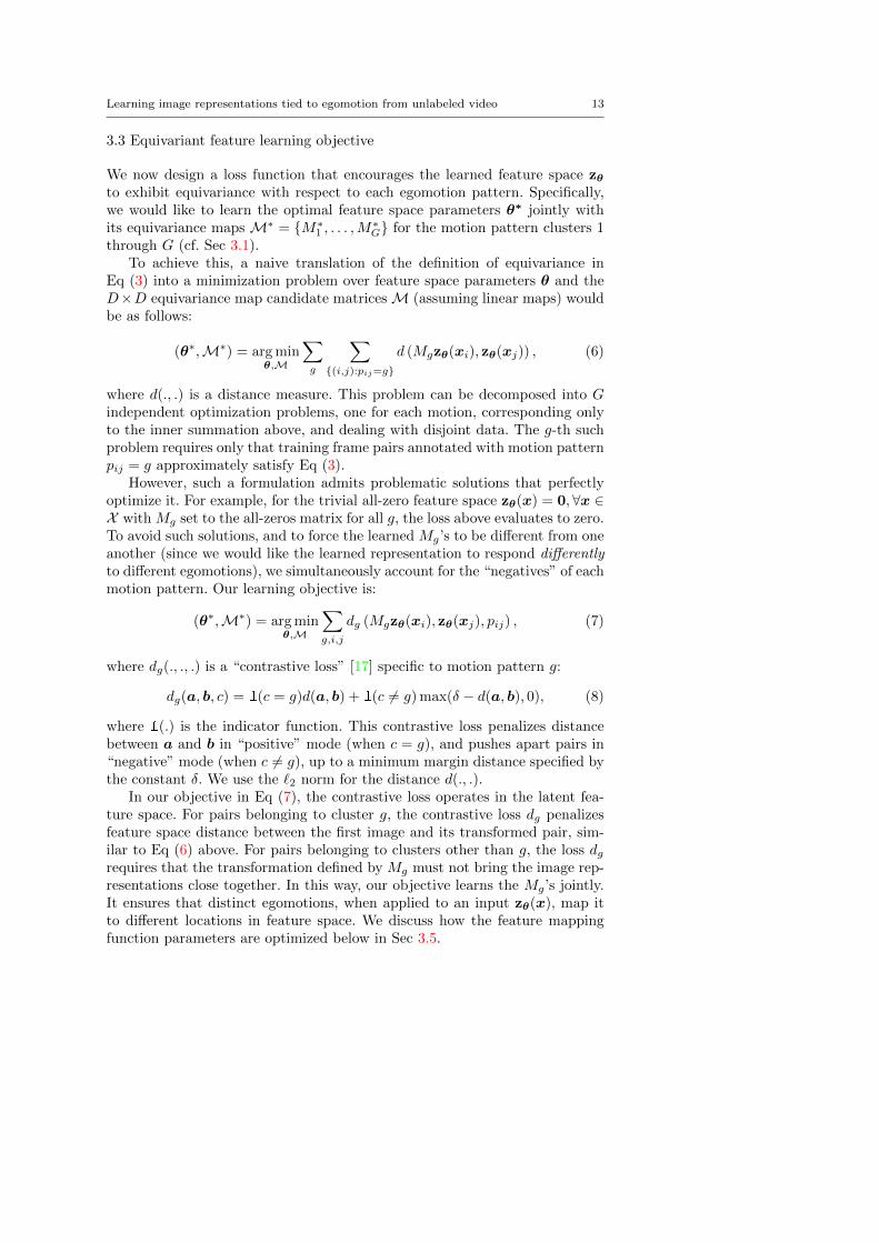
Fig. 5 Training setup for discrete egomotions: (top) a two-stack “Siamese network” pro-cesses video frame pairs identically before optimizing the equivariance loss of Eq (7), and(bottom) a third layer stack simultaneously processes class-labeled images to optimize thesupervised recognition softmax loss as in Eq (14). See Sec 4.1 for exact network specifica-tions.
moti
on-p
att
ern
image p
air
s
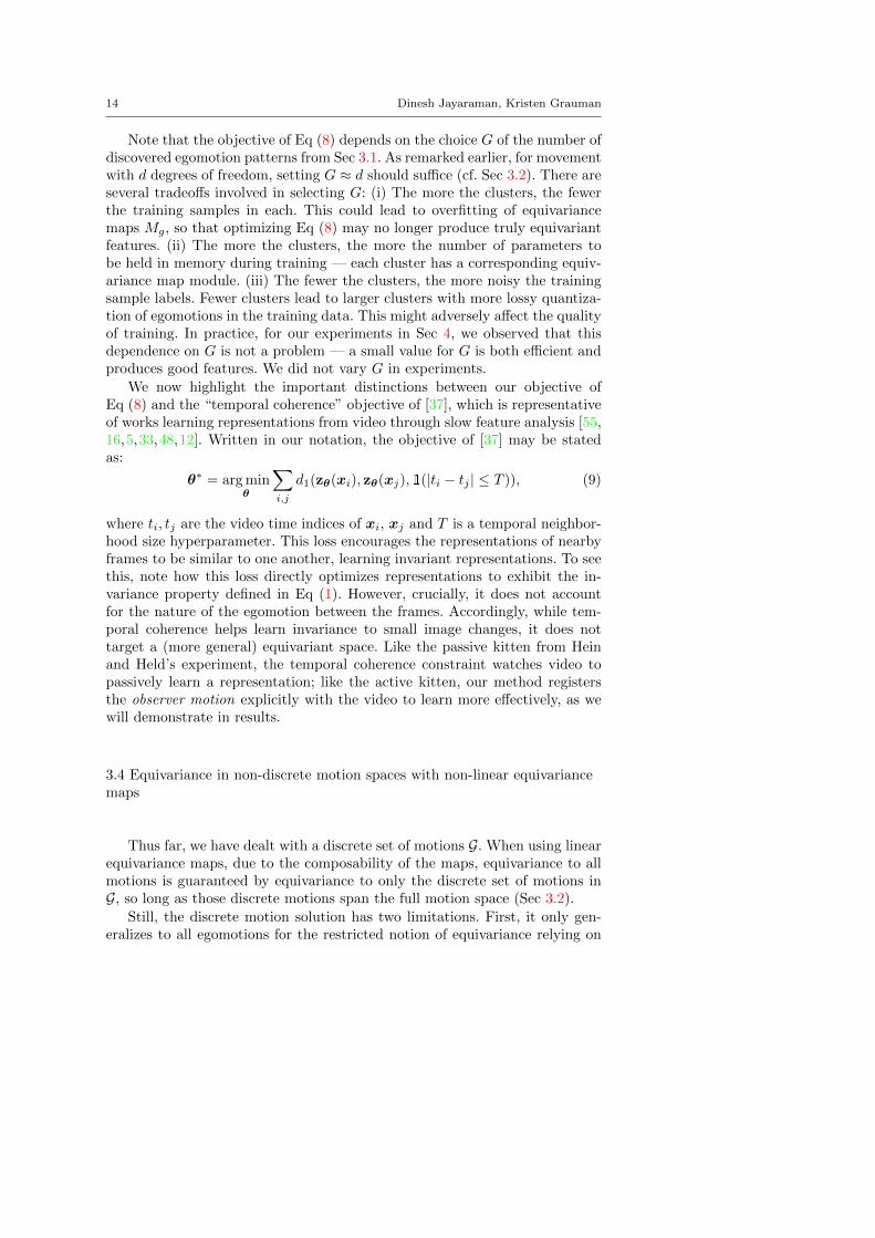
Fig. 6 Unsupervised training setup for the “non-discrete” variant Eq (13) of the equivari-ance objective. First, layer stacks with tied weights, representing the feature mapping zθ tobe learned, process video frame pairs identically to embed them into a feature space. In thisspace, an equivariance mapping function M(.) acts on the first frame and camera egomotionvector g to attempt to predict the second frame. See Fig 7 for the architecture of M(.), andSec 4.1 for further details. When used in a regularization setup with labeled data L, a thirdstack of layers may be added as in Fig 5 to compute the classification loss.
ture of the function M(.) and how it is trained, are specified in Sec 3.5 andSec 4.1.
This non-discretized motion and non-linear equivariance formulation allowsan easy way to control the strength of the equivariance objective. The morecomplex the class of functions modeled by M(.), the weaker the notion ofequivariance that is imposed upon the learned feature space. Moreover, it doesnot require discarding fine-grained information among the egomotion labels,as in the discrete motion case. We evaluate the impact of these conceptualdifferences, in experiments (Sec 4.4).
3.5 Form of the feature mapping function zθ(.)
For the mapping zθ(.), we use a convolutional neural network architecture, sothat the parameter vector θ now represents the layer weights. We start with thediscrete egomotions variant of our method. Let Led denote the equivarianceloss of Eq (7) based on discretized egomotions. Led is optimized by sharingthe weight parameters θ among two identical stacks of layers in a “Siamese”network [4,17,37], as shown in the top two rows of Fig 5. Video frame pairsfrom U are fed into these two stacks. Both stacks are initialized with identicalrandom weights, and identical gradients are passed through them in every
Learning image representations tied to egomotion from unlabeled video 17
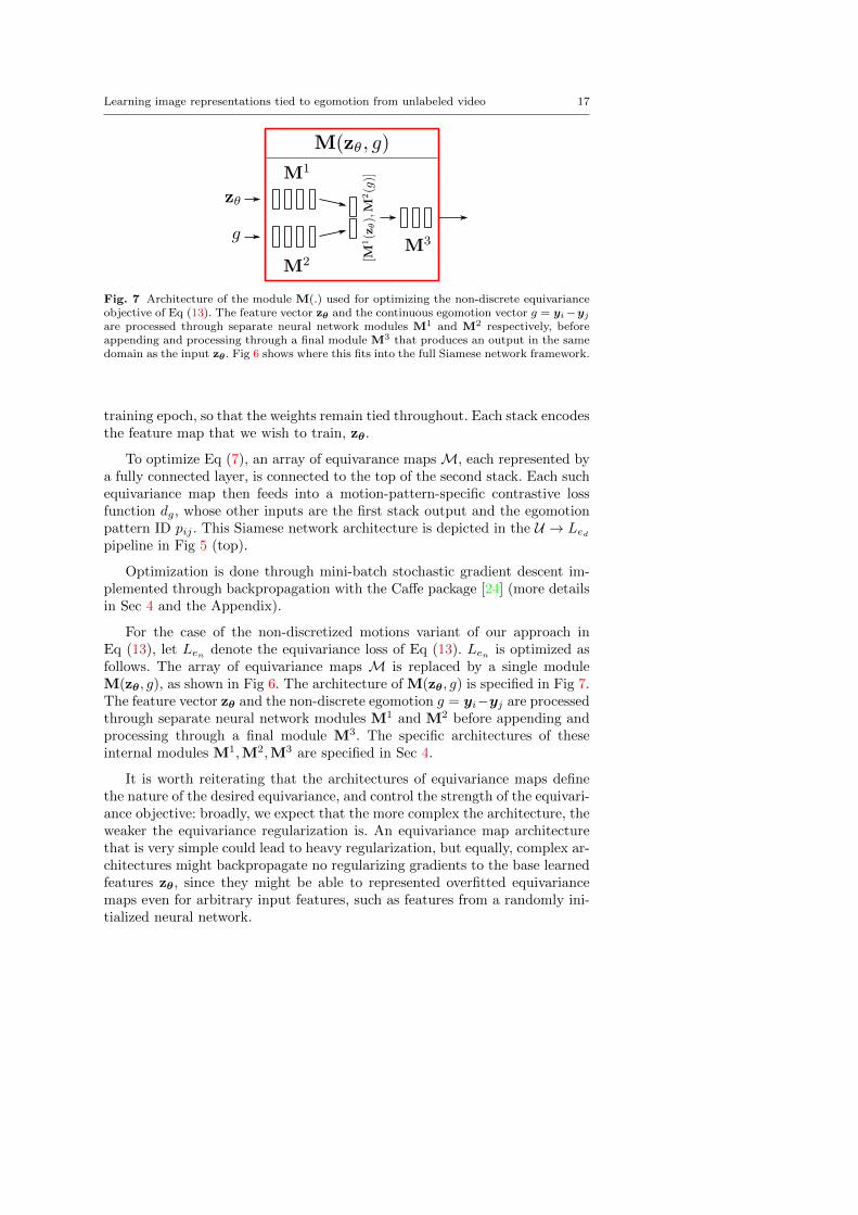
Fig. 7 Architecture of the module M(.) used for optimizing the non-discrete equivarianceobjective of Eq (13). The feature vector zθ and the continuous egomotion vector g = yi−yjare processed through separate neural network modules M1 and M2 respectively, beforeappending and processing through a final module M3 that produces an output in the samedomain as the input zθ . Fig 6 shows where this fits into the full Siamese network framework.
training epoch, so that the weights remain tied throughout. Each stack encodesthe feature map that we wish to train, zθ.
To optimize Eq (7), an array of equivarance maps M, each represented bya fully connected layer, is connected to the top of the second stack. Each suchequivariance map then feeds into a motion-pattern-specific contrastive lossfunction dg, whose other inputs are the first stack output and the egomotionpattern ID pij . This Siamese network architecture is depicted in the U → Led
pipeline in Fig 5 (top).
Optimization is done through mini-batch stochastic gradient descent im-plemented through backpropagation with the Caffe package [24] (more detailsin Sec 4 and the Appendix).
For the case of the non-discretized motions variant of our approach inEq (13), let Len denote the equivariance loss of Eq (13). Len is optimized asfollows. The array of equivariance maps M is replaced by a single moduleM(zθ, g), as shown in Fig 6. The architecture of M(zθ, g) is specified in Fig 7.The feature vector zθ and the non-discrete egomotion g = yi−yj are processedthrough separate neural network modules M1 and M2 before appending andprocessing through a final module M3. The specific architectures of theseinternal modules M1,M2,M3 are specified in Sec 4.
It is worth reiterating that the architectures of equivariance maps definethe nature of the desired equivariance, and control the strength of the equivari-ance objective: broadly, we expect that the more complex the architecture, theweaker the equivariance regularization is. An equivariance map architecturethat is very simple could lead to heavy regularization, but equally, complex ar-chitectures might backpropagate no regularizing gradients to the base learnedfeatures zθ, since they might be able to represented overfitted equivariancemaps even for arbitrary input features, such as features from a randomly ini-tialized neural network.
18 Dinesh Jayaraman, Kristen Grauman
3.6 Applying learned equivariant representations to recognition tasks
While we have thus far described our formulation for generic equivariant im-age representation learning, our hypothesis is that representations trained asabove will facilitate high-level visual tasks such as recognition. One way tosee this is by observing that equivariant representations expose camera andobject pose-related parameters to a recognition algorithm, which may thenaccount for this critical information while making predictions. For instance,a feature space that embeds knowledge of how objects change under differentviewpoints/manipulations may allow a recognition system to hallucinate newviews (in that feature space) of an object to improve performance.
More generally, recall the intuitions gained from the view prediction taskillustrated in Fig 2. As discussed in Sec 1, acquiring the ability to hallucinatefuture views in severely underdetermined situations requires mastery of com-plex visual skills like depth, 3D geometry, semantics, and context. Therefore,our equivariance formulation of this view prediction task within the learnedfeature space induces the development of these ancillary high-level skills, whichare transferable to other high-level tasks like object or scene recognition.
Suppose that in addition to the ego-pose annotated pairs U we are alsogiven a small set of Nl class-labeled static images, L = {(xk, ck}Nl
k=1, whereck ∈ {1, . . . , C}. We may now adapt our equivariance formulation to enable thetraining of a recognition pipeline on L. In our experiments, we do this in twosettings, purely unsupervised feature extraction (Sec 4.4), and unsupervisedregularization of the supervised recognition task (Sec 4.5). We now describethe approaches for these two settings in detail.
In both of the scenarios below, note that neither the supervised trainingdata L nor the testing data for recognition are required to have any associatedsensor data. Thus, our features are applicable to standard image recognitiontasks.
3.6.1 Adapting unsupervised equivariant features for recognition
In the unsupervised setting, we first train representations by optimizing theequivariance objective of Eq (7) (or Eq (13) for the non-discrete case). We thendirectly represent the class-labeled images from L in our learned equivariantfeature space. These features may then be input to a generic machine learn-ing pipeline, such as a k-nearest neighbor classifier, that is to be trained forrecognition using labeled data L. Alternatively, the weights learned in the net-work may be finetuned using the labeled data L, producing a neural networkclassifier.
This setting allows us to test if optimizing neural networks only for equiv-ariant representations, with no explicit discriminative component in the lossfunction, still produces discriminative representations. Aside from testing thepower of our equivariant feature learning objective in isolation, this setting al-lows a nice modularity between the feature learning step and category learningstep. In particular, when learned prior to any recognition task, our features
Learning image representations tied to egomotion from unlabeled video 19
can be used for easy “off-the shelf” testing of the unsupervised neural net-work directly as a feature extractor for new tasks. The user does not need tosimultaneously optimize the embedding parameters and classifier parametersspecific to his task. Moreoever, it requires no more computational resourcesthan for the Siamese paired network scheme described in Sec 3.5 for learningequivariant representations.
3.6.2 Unsupervised equivariance regularization for recognition
Alternatively, we may jointly train representations for equivariance, as wellas for discriminative ability geared towards a target recognition task. Let Led
denote the unsupervised equivariance loss of Eq (7). We can integrate ourunsupervised feature learning scheme with the recognition task, by optimizinga misclassification loss together with Led . Let W be a C×D matrix of classifierweights. We solve jointly for W and the maps M:
(θ∗,W ∗,M∗) = argminθ,W,M
Lc(θ,W,L) + λLe(θ,M,U), (14)
where Lc denotes the softmax loss over the learned features:
Lc(W,L) = − 1
Nl
Nl∑i=1
log(σck(Wzθ(xi)), (15)
and σck(.) is the softmax probability of the correct class.
σci(pi) = exp(pci)/
C∑c=1
exp(pc). (16)
The regularizer weight λ in Eq (14) is a hyperparameter.
In this setting, the unsupervised egomotion equivariance loss encodes aprior over the feature space that can improve performance on the supervisedrecognition task with limited training examples.
To optimize Eq (14), in addition to the Siamese net that minimizes Le asabove, the supervised softmax loss is minimized through a third replica of thezθ layer stack with weights tied to the two Siamese networks stacks. Labelledimages from L are fed into this stack, and its output is fed into a softmax layerwhose other input is the class label. So while this is a more complete frameworkfor applying our equivariant representations to recognition tasks, it is alsomore computationally intensive; it requires more memory, more computationper iteration, and more iterations for convergence due to the more complexobjective function. The complete scheme is depicted in Fig 5.
20 Dinesh Jayaraman, Kristen Grauman
ObjectGuesses Guesses
View 1
View 2
Object
cup?
bowl?
pan?
cup
cup?
bowl?
pan?
pan
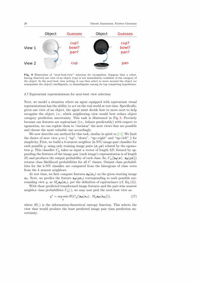
Fig. 8 Illustration of “next-best-view” selection for recognition. Suppose that a robot,having observed one view of an object (top) is not immediately confident of the category ofthe object. In the next-best view setting, it can then select to move around the object (ormanipulate the object) intelligently, to disambiguate among its top competing hypotheses.
3.7 Equivariant representations for next-best view selection
Next, we model a situation where an agent equipped with equivariant visualrepresentations has the ability to act on the real world at test time. Specifically,given one view of an object, the agent must decide how to move next to helprecognize the object, i.e., which neighboring view would best reduce objectcategory prediction uncertainty. This task is illustrated in Fig 8. Preciselybecause our features are equivariant (i.e., behave predictably) with respect toegomotion, we can exploit them to “envision” the next views that are possibleand choose the most valuable one accordingly.
We now describe our method for this task, similar in spirit to [51]. We limitthe choice of next view g to { “up”, “down”, “up+right” and “up+left” } forsimplicity. First, we build a k-nearest neighbor (k-NN) image-pair classifier foreach possible g, using only training image pairs (x, gx) related by the egomo-tion g. This classifier Cg takes as input a vector of length 2D, formed by ap-pending the features of the image pair (each image’s representation is of lengthD) and produces the output probability of each class. So, Cg([zθ(x), zθ(gx)])returns class likelihood probabilities for all C classes. Output class probabil-ities for the k-NN classifier are computed from the histogram of class votesfrom the k nearest neighbors.
At test time, we first compute features zθ(x0) on the given starting imagex0. Next, we predict the feature zθ(gx0) corresponding to each possible sur-rounding view g, as Mgzθ(x0), per the definition of equivariance (cf. Eq (3)).
With these predicted transformed image features and the pair-wise nearestneighbor class probabilities Cg(.), we may now pick the next-best view as:
g∗ = argming
H(Cg([zθ(x0), Mgzθ(x0)])), (17)
where H(.) is the information-theoretical entropy function. This selects theview that would produce the least predicted image pair class prediction un-certainty.
Learning image representations tied to egomotion from unlabeled video 21
4 Experiments
We validate our approach on three public datasets and compare to multipleexisting methods. The main questions we address in the experiments are: (i)quantitatively, how well is equivariance preserved in our learned embedding?(Sec 4.2); (ii) qualitatively, can we see the egomotion consistency of embeddedimage pairs? (Sec 4.3); (iii) when learned entirely without supervision, howuseful are our method’s features for recognition tasks? (Sec 4.4); (iv) whenused as a regularizer for a classification loss, how effective are our method’sfeatures for recognition tasks? (Sec 4.5); and (v) how effective are the learnedequivariant features for next-best view selection in an active recognition sce-nario? (Sec 4.6).
Throughout, we compare the following methods:
– clsnet: A neural network trained only from the supervised samples witha softmax loss.
– temporal: The temporal coherence approach of [37], which regularizes theclassification loss with Eq (9) setting the distance measure d(.) to the `1distance in d1. This method aims to learn invariant features by exploitingthe fact that adjacent video frames should not change too much.
– drlim: The approach of [17], which also regularizes the classification losswith Eq (9), but setting d(.) to the `2 distance in d1.
– lsm: The “learning to see by moving” (LSM) approach of [2], proposedindependently and concurrently with our method, which also exploits videowith accompanying egomotion for unsupervised representation learning.lsm uses egomotion in an alternative approach to ours; it trains a neuralnetwork to predict the observer egomotion g, given views x and gx, beforeand after the motion. In our experiments, we use the publicly availableKITTI-trained model provided by the authors.
– equiv: Our egomotion equivariant feature learning approach, as definedby the objective of Eq (7).
– equiv+drlim: Our approach augmented with temporal coherence regu-larization ([17]).
– equiv+drlim (non-discrete): The non-discrete motion variant of our ap-proach as defined by the objective of Eq (12), augmented with temporalcoherence regularization.6
All of these baselines are identically augmented with a classification loss forthe regularization-based experiments in Sec 4.2, 4.5 and 4.6. temporal anddrlim are the most pertinent baselines for validating our idea of exploitingegomotion for visual learning, because they, like us, use contrastive loss-based
6 Note that we do not test equiv (non-discrete) i.e., the non-discrete formulation of Eq (13)in isolation. This is because Eq (13) specifies a non-contrastive loss that would result incollapsed feature spaces (such as zθ = 0∀x) if optimized in isolation. To overcome thisdeficiency, we optimize this non-discrete equivariance loss only in conjunction with thecontrastive drlim loss in the equiv+drlim (non-discrete) approach.
22 Dinesh Jayaraman, Kristen Grauman
formulations, but represent the popular “slowness”-based family of techniques([55,5,16,33,12]) for unsupervised feature learning from video, which, unlikeour approach, are passive. In addition, our results against lsm evaluate thestrength of our egomotion-equivariance formulation against the alternativeapproach of [2].
4.1 Experimental setup details
Recall that in the fully unsupervised mode, our method trains with pairsof video frames annotated only by their ego-poses in U . In the supervisedmode, when applied to recognition, our method additionally has access to aset of class-labeled images in L. Similarly, the baselines all receive a pool ofunsupervised data and supervised data. We now detail the data composingthese two sets.
Unsupervised datasets We consider two unsupervised datasets, NORB andKITTI, to compose the unlabeled video pools U augmented with egomotion.
– NORB [29]: This dataset has 24,300 96×96-pixel images of 25 toys cap-tured by systematically varying camera pose. We generate a random 67%-33% train-validation split and use 2D ego-pose vectors y consisting of cam-era elevation and azimuth. Because this dataset has discrete ego-pose varia-tions, we consider two egomotion patterns, i.e, G = 2 (cf. Sec 3.1): one stepalong elevation and one step along azimuth. For equiv, we use all avail-able positive pairs for each of the two motion patterns from the trainingimages, yielding a Nu = 45, 417-pair training set. For drlim and tempo-ral, we create a 50,000-pair training set (positives to negatives ratio 1:3).Pairs within one step (elevation and/or azimuth) are treated as “temporalneighbors”, as in the turntable results of [17,37].
– KITTI [13,14]: This dataset contains videos with registered GPS/IMUsensor streams captured on a car driving around four types of areas (loca-tion classes): “campus”, “city”, “residential”, “road”. We generate a ran-dom 67%-33% train-validation split and use 2D ego-pose vectors consistingof “yaw” and “forward position” (integral over “forward velocity” sensoroutputs) from the sensors. We discover egomotion patterns pij (cf. Sec 3.1)on frame pairs ≤ 1 second apart. We compute 6 clusters and automati-cally retain the G = 3 with the largest motions, which upon inspectioncorrespond to “forward motion/zoom”, “right turn”, and “left turn” (seeFig 4). For equiv, we create a Nu = 47, 984-pair training set with 11,996positives. For drlim and temporal, we create a 98,460-pair training setwith 24,615 “temporal neighbor” positives sampled ≤2 seconds apart.7
Of the various KITTI cameras that simultaneously capture video, we usethe feed from “camera 0” (see [14] for details) in our expriments. For our
7 For fairness, the training frame pairs for each method are drawn from the same startingset of KITTI training videos.
Learning image representations tied to egomotion from unlabeled video 23
SUN imagesStatic web images
397 scene categories
NORB imagesOrbits of toy images
Egomotions:
elevation, azimuth
KITTI videoCar platform
Egomotions:
yaw,
forward motion
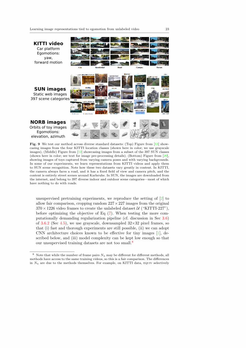
Fig. 9 We test our method across diverse standard datasets: (Top) Figure from [13] show-casing images from the four KITTI location classes (shown here in color; we use grayscaleimages), (Middle) Figure from [52] showcasing images from a subset of the 397 SUN classes(shown here in color; see text for image pre-processing details). (Bottom) Figure from [29],showing images of toys captured from varying camera poses and with varying backgrounds.In some of our experiments, we learn representations from KITTI videos and apply themto SUN scene recognition. Note how these two datasets vary greatly in content. In KITTI,the camera always faces a road, and it has a fixed field of view and camera pitch, and thecontent is entirely street scenes around Karlsruhe. In SUN, the images are downloaded fromthe internet, and belong to 397 diverse indoor and outdoor scene categories—most of whichhave nothing to do with roads.
unsupervised pretraining experiments, we reproduce the setting of [2] toallow fair comparison, cropping random 227×227 images from the original370× 1226 video frames to create the unlabeled dataset U (“KITTI-227”),before optimizing the objective of Eq (7). When testing the more com-putationally demanding regularization pipeline (cf. discussion in Sec 3.6)of 3.6.2 (Sec 4.5), we use grayscale, downsampled 32×32 pixel frames, sothat (i) fast and thorough experiments are still possible, (ii) we can adoptCNN architecture choices known to be effective for tiny images [1], de-scribed below, and (iii) model complexity can be kept low enough so thatour unsupervised training datasets are not too small.8
8 Note that while the number of frame pairs Nu may be different for different methods, allmethods have access to the same training videos, so this is a fair comparison. The differencesin Nu are due to the methods themselves. For example, on KITTI data, equiv selectively
24 Dinesh Jayaraman, Kristen Grauman
Supervised datasets In our recognition experiments, we consider three super-vised datasets L. These datasets allow us to test our approach’s impact forthree distinct recognition tasks for static images: object instance recognition,location recognition, and scene recognition. The supervised datasets are:
– NORB: We select six images from each of the C = 25 object trainingsplits at random to create instance recognition training data.
– KITTI: We select four images from each of the C = 4 location classtraining splits at random to create location recognition training data.
– SUN [52]: We select six images for each of C = 397 scene categoriesat random from the standard training dataset to create scene recognitiontraining data, unless otherwise stated. We preprocess them identically tothe KITTI images above for all experiments. For the purely unsupervisedexperiments, we follow the setting of [2], resizing images to 256×256 beforecropping random 227× 227 regions (“SUN-227”).
We keep all the supervised datasets small, since unsupervised feature learn-ing should be most beneficial when labeled data is scarce. This corresponds tohandling categorization problems in the “long tail”. Note that while the videoframes of the unsupervised datasets U are associated with ego-poses, the staticimages of L have no such auxiliary data.
Network architectures and optimization We now discuss the neural networkarchitectures used for the base network zθ and the equivariance maps in variousexperimental settings.
For NORB, zθ is a fully connected network: 20 full-ReLU→ D =100 fullfeature units. Mg is a single fully connected layer Linear(100,100). These areschematically depicted in Fig 10 (top row).
For KITTI, the base neural network zθ closely follows the cuda-convnet [1]recommended CIFAR-10 architecture: 32 Conv(5x5)-MaxPool(3x3)-ReLU →32 Conv(5x5)-ReLU-AvgPool(3x3) → 64 Conv(5x5)-ReLU-AvgPool(3x3) →D =64 full feature units. The equivariance map Mg is a single fully con-nected layer Linear(64,64), which takes in 64-dimensional zθ(x) as input, andproduces 64-dimensional Mgzθ(x) as output. Fig 10 (middle row) presentsschematics of these architectures.
For experiments with KITTI-227 and SUN-227, we follow the standardAlexNet architecture, augmented for fast training with batch normalization [20](before every layer with learnable weights - conv1-5, fc6 ). We truncate theAlexNet architecture at the first fully connected layer, fc6, treating its outputas the feature representation zθ. For equiv+drlim(discrete), the equivariancemap modules Mg have the architecture: input → Linear(4096,128) → ReLU→ Linear(128,4096), that produces a feature in the original 4096-dim featurespace.9 For equiv+drlim(non-discrete), the architecture of the equivariancemap module M(.) follows the outline in Sec 3.5 and Fig 7. Specifically,
uses frame pairs corresponding to large motions (Sec 3.1), so even given the same startingvideos, it is restricted to using a smaller number of frame pairs than drlim and temporal.
9 We do not use a straightforward fully connected layer Linear(4096,4096) as this woulddrastically increase the number of network parameters, and possibly cause overfitting of Mg ,
Learning image representations tied to egomotion from unlabeled video 25K
ITTI-
227
SU
N-2
27
4096128
fully connected
ReLU
fully connected
conv1
conv2
conv3
conv4
conv5
fc6
128
128
2564096
fully connected
ReLU
fully connected
ReLU
fully connectedconcatenate
KIT
TI
SU
N
max-pool
(3x3, stride2)
ReLU
ReLU
avg-pool
(3x3, stride2)
5
5
1 32
32
32
32
15
15
7
7
5
5
64
64
3
3
64
fully
connected
ReLU
avg-pool
(3x3)
5
5
64
fully
connected
NO
RB
96
96
20 100
204096
fully connected
ReLU
fully connected
100
fully
connected
(AlexNet architecture)
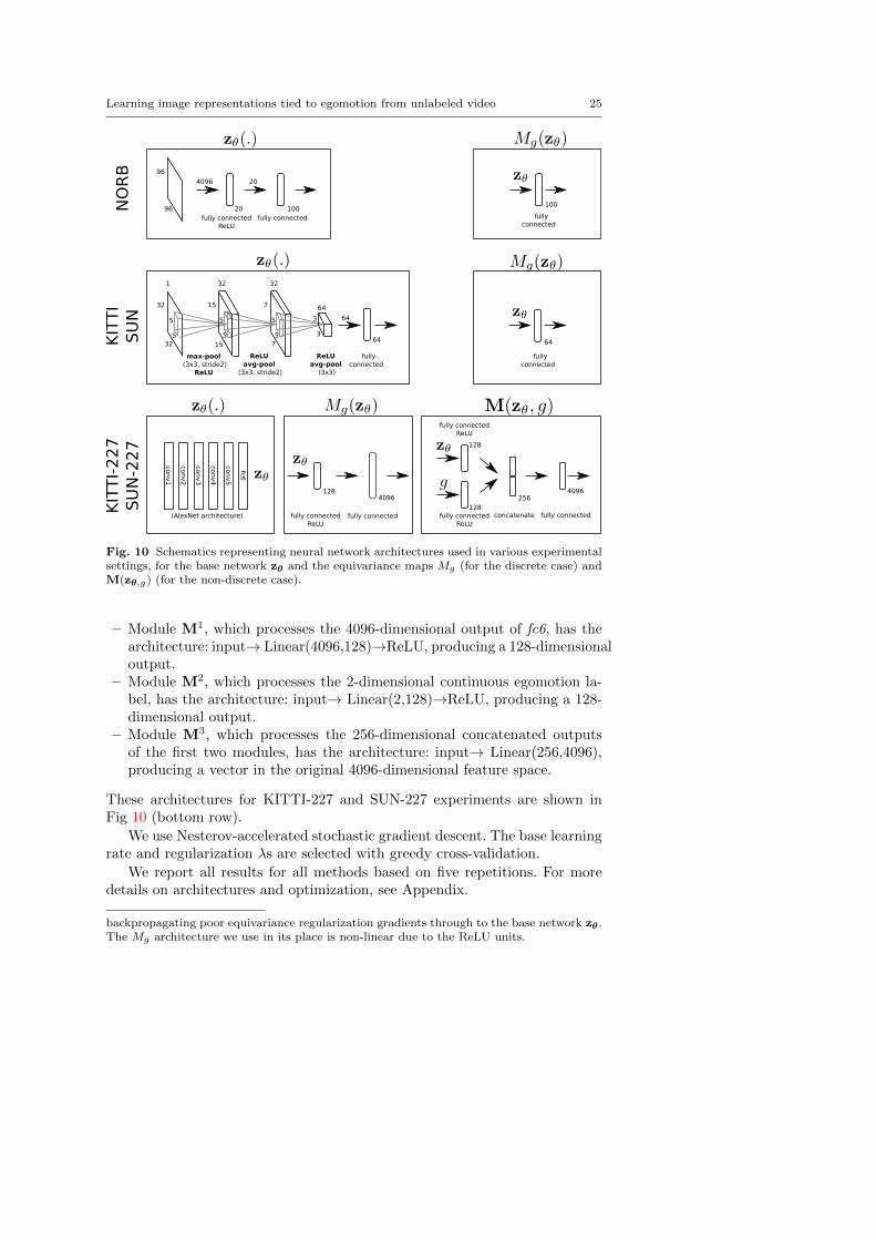
Fig. 10 Schematics representing neural network architectures used in various experimentalsettings, for the base network zθ and the equivariance maps Mg (for the discrete case) andM(zθ,g) (for the non-discrete case).
– Module M1, which processes the 4096-dimensional output of fc6, has thearchitecture: input→ Linear(4096,128)→ReLU, producing a 128-dimensionaloutput.
– Module M2, which processes the 2-dimensional continuous egomotion la-bel, has the architecture: input→ Linear(2,128)→ReLU, producing a 128-dimensional output.
– Module M3, which processes the 256-dimensional concatenated outputsof the first two modules, has the architecture: input→ Linear(256,4096),producing a vector in the original 4096-dimensional feature space.
These architectures for KITTI-227 and SUN-227 experiments are shown inFig 10 (bottom row).
We use Nesterov-accelerated stochastic gradient descent. The base learningrate and regularization λs are selected with greedy cross-validation.
We report all results for all methods based on five repetitions. For moredetails on architectures and optimization, see Appendix.
backpropagating poor equivariance regularization gradients through to the base network zθ .The Mg architecture we use in its place is non-linear due to the ReLU units.
26 Dinesh Jayaraman, Kristen Grauman
4.2 Quantitative analysis: equivariance measurement
First, we test the learned features for equivariance. Equivariance is measuredseparately for each egomotion g through the normalized error ρg:
ρg = E
[‖M ′
gzθ(x)− zθ(gx)‖2‖zθ(x)− zθ(gx)‖2
], (18)
where E[.] denotes the empirical mean, M′
g is the equivariance map, andρg = 0 would signify perfect equivariance. To understand this error measure,we start by noting that the numerator is directly related to the definition ofequivariance in Eq (3): zθ(gx) ≈ Mgzθ(x). Thus, the numerator alone consti-tutes the most straightforward measure of equivariance error. However, thisterm depends on the scale of the feature representation, which may vary be-tween methods. So, rather than measure the distance between the transformedand ground truth features directly, ρg measures the ratio by which M ′
g reducesthe distance between zθ(gx) and zθ(x). The denominator and numerator inEq (18) are therefore the distance between the representations of original andtransformed images, respectively before and after applying the equivariancemap. The normalized error ρg is the empirical mean of this distance reductionratio across all samples.
We closely follow the equivariance evaluation approach of [30] to solvefor the equivariance maps of features produced by each compared methodon held-out validation data, before computing ρg. Such maps are producedexplicitly by our method, but not the baselines. Thus, as in [30], we computetheir maps10 by solving a least squares minimization problem based on thedefinition of equivariance in Eq (3):
M ′g = argmin
M
∑m(yi,yj)=g
‖zθ(xi)−Mzθ(xj)‖2. (19)
The equivariance maps M ′g computed as above are used to compute the nor-
malized errors ρg as in Eq (18). M ′g and ρg are computed on disjoint subsets
of the validation image pairs.We test both (i) “atomic” egomotions matching those provided in the
training pairs (i.e, “up” 5◦and “down” 20◦) and (ii) composite egomotions(“up+right”, “up+left”, “down+right”). The latter lets us verify that ourmethod’s equivariance extends beyond those motion patterns used for train-ing (cf. Sec 3.2).
First, as a sanity check, we quantify equivariance for the unsupervised lossof Eq (7) in isolation, i.e, learning with only U . Our equiv method’s aver-age ρg error is 0.0304 and 0.0394 for atomic and composite egomotions inNORB, respectively. In comparison, drlim—which promotes invariance, not
10 For uniformity, we do the same recovery of M ′g for our method; our results are similar
either way.
Learning image representations tied to egomotion from unlabeled video 27
Motion types → atomic compositeMethods ↓ “up (u)” “right (r)” avg. “u+r” “u+l” “d+r” avg.
random 1.0000 1.0000 1.0000 1.0000 1.0000 1.0000 1.0000clsnet 0.9276 0.9202 0.9239 0.9222 0.9138 0.9074 0.9145temporal [37] 0.7140 0.8033 0.7587 0.8089 0.8061 0.8207 0.8119drlim [17] 0.5770 0.7038 0.6404 0.7281 0.7182 0.7325 0.7263
equiv 0.5328 0.6836 0.6082 0.6913 0.6914 0.7120 0.6982equiv+drlim 0.5293 0.6335 0.5814 0.6450 0.6460 0.6565 0.6492
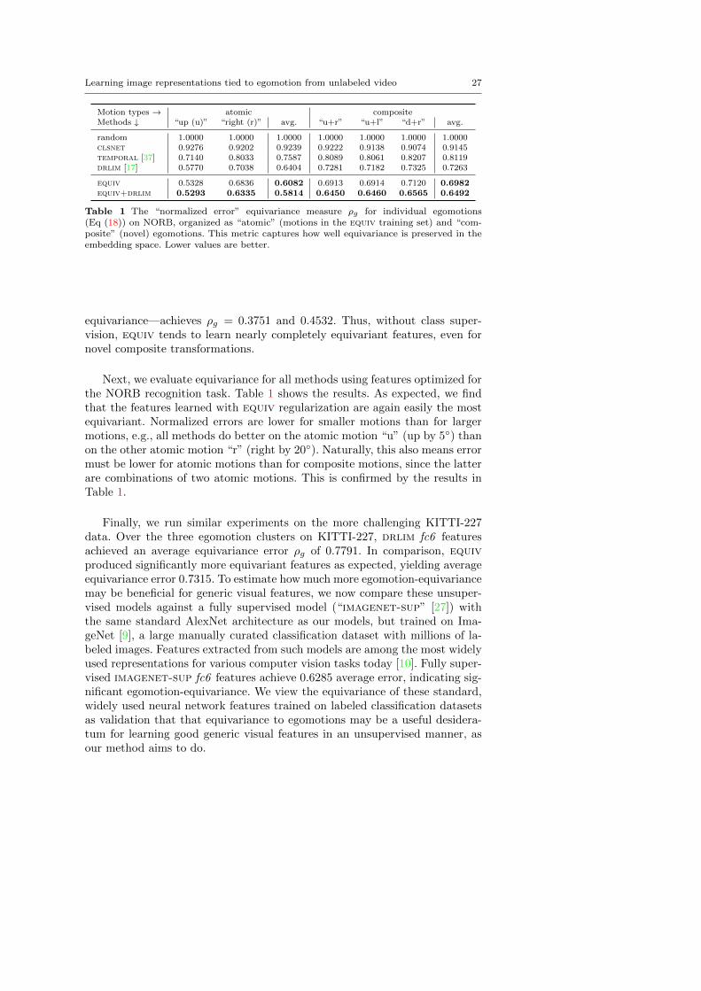
Table 1 The “normalized error” equivariance measure ρg for individual egomotions(Eq (18)) on NORB, organized as “atomic” (motions in the equiv training set) and “com-posite” (novel) egomotions. This metric captures how well equivariance is preserved in theembedding space. Lower values are better.
equivariance—achieves ρg = 0.3751 and 0.4532. Thus, without class super-vision, equiv tends to learn nearly completely equivariant features, even fornovel composite transformations.
Next, we evaluate equivariance for all methods using features optimized forthe NORB recognition task. Table 1 shows the results. As expected, we findthat the features learned with equiv regularization are again easily the mostequivariant. Normalized errors are lower for smaller motions than for largermotions, e.g., all methods do better on the atomic motion “u” (up by 5◦) thanon the other atomic motion “r” (right by 20◦). Naturally, this also means errormust be lower for atomic motions than for composite motions, since the latterare combinations of two atomic motions. This is confirmed by the results inTable 1.
Finally, we run similar experiments on the more challenging KITTI-227data. Over the three egomotion clusters on KITTI-227, drlim fc6 featuresachieved an average equivariance error ρg of 0.7791. In comparison, equivproduced significantly more equivariant features as expected, yielding averageequivariance error 0.7315. To estimate how much more egomotion-equivariancemay be beneficial for generic visual features, we now compare these unsuper-vised models against a fully supervised model (“imagenet-sup” [27]) withthe same standard AlexNet architecture as our models, but trained on Ima-geNet [9], a large manually curated classification dataset with millions of la-beled images. Features extracted from such models are among the most widelyused representations for various computer vision tasks today [10]. Fully super-vised imagenet-sup fc6 features achieve 0.6285 average error, indicating sig-nificant egomotion-equivariance. We view the equivariance of these standard,widely used neural network features trained on labeled classification datasetsas validation that that equivariance to egomotions may be a useful desidera-tum for learning good generic visual features in an unsupervised manner, asour method aims to do.
28 Dinesh Jayaraman, Kristen Grauman
+
query pair NN (ours) NN (pixel)+
+
KITTI frame pairs
query pair NN (ours) NN (pixel)
NORB frame pairs
query pair NN (ours) NN (pixel)
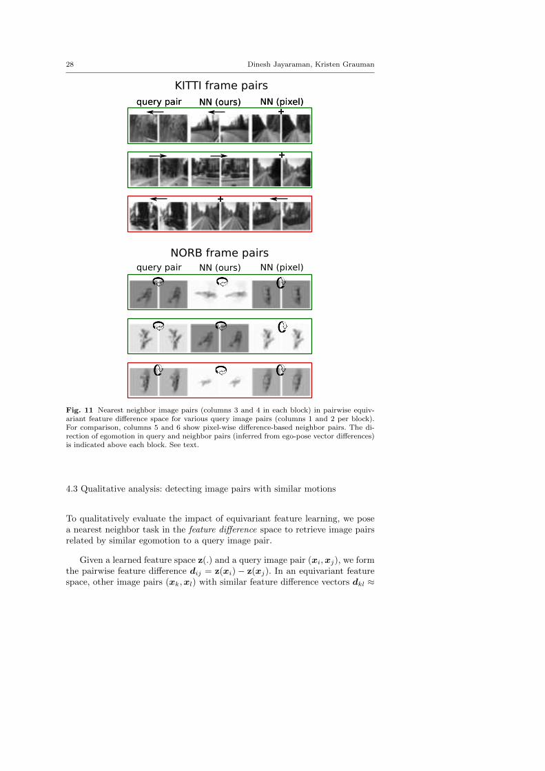
Fig. 11 Nearest neighbor image pairs (columns 3 and 4 in each block) in pairwise equiv-ariant feature difference space for various query image pairs (columns 1 and 2 per block).For comparison, columns 5 and 6 show pixel-wise difference-based neighbor pairs. The di-rection of egomotion in query and neighbor pairs (inferred from ego-pose vector differences)is indicated above each block. See text.
4.3 Qualitative analysis: detecting image pairs with similar motions
To qualitatively evaluate the impact of equivariant feature learning, we posea nearest neighbor task in the feature difference space to retrieve image pairsrelated by similar egomotion to a query image pair.
Given a learned feature space z(.) and a query image pair (xi,xj), we formthe pairwise feature difference dij = z(xi) − z(xj). In an equivariant featurespace, other image pairs (xk,xl) with similar feature difference vectors dkl ≈
Learning image representations tied to egomotion from unlabeled video 29
dij would be likely to be related by similar egomotion to the query pair.11 Thiscan also be viewed as an analogy completion task, xi : xj = xk :?, where theright answer xl must be computed by applying the unknown transformationpij to xk.
Fig 11 shows examples from KITTI (top) and NORB (bottom). For avariety of query pairs, we show the top neighbor pairs in the equiv space, aswell as in pixel-difference space for comparison. Overall they visually confirmthe desired equivariance property: neighbor-pairs in equiv’s difference spaceexhibit a similar transformation (turning, zooming, etc.), whereas those in theoriginal image space often do not. Consider the first NORB example (firstrow among NORB examples), where pixel distance, perhaps dominated bythe lighting, identifies a wrong egomotion match, whereas our approach findsa correct match, despite the changed object identity, starting azimuth, lightingetc. The red boxes show failure cases. For instance, in the last KITTI example(third row), large foreground motion of a truck in the query image pair causesour method to wrongly miss the rotational motion.
4.4 Unsupervised feature extraction and finetuning for classification
Next, we present experiments to test whether useful visual features may betrained in neural networks by minimizing only the unsupervised equivarianceloss of Eq (7), using no labeled samples. We follow the approach described inSec 3.6.1.
As discussed before, this setting tests the power of our equivariant featurelearning objective in isolation, and offers several advantages: (i) It has lowermemory and computational requirements, since there is no need for a thirdstack of layers dedicated to classification (Sec 3.5, Fig 5). (ii) It allows easyoff-the-shelf testing of the unsupervised neural network either directly as a fea-ture extractor for new tasks, or as a “pretrained” network to be fine-tuned fornew tasks (iii) It gets rid of the regularization λ of Eq (14), thus leaving fewerhyperparameters to optimize. These advantages allow relatively fast experi-mentation with large neural networks to test our purely supervised pipeline.We therefore perform experiments on large 227 × 227 images for most of theremainder of this section.
For these experiments, each layer stack follows the standard AlexNet ar-chitecture [27] for the layer stacks in these experiments, treating the output ofthe first fully connected layer, fc6, as the feature representation zθ (as shownin Fig 10). Both the 227×227 image resolution and network architecture allowus to test our method with identical settings against a concurrent and inde-pendently proposed approach for unsupervised representation learning fromvideo+egomotion [2], lsm. We compare the features produced by our methodagainst baselines under two conditions: nearest neighbor classification, and
11 Note that in our model of equivariance, this is not strictly true, since the pair-wisedifference vector Mgzθ(x)−zθ(x) need not actually be consistent across images x. However,for small motions and linear maps Mg , this still holds approximately, as we show empirically.
30 Dinesh Jayaraman, Kristen Grauman
finetuning for classification. In the rest of this subsection, we first presentboth these settings in Sec 4.4.1 and Sec 4.4.2, before discussing their resultstogether in Sec 4.4.3.
4.4.1 Nearest neighbor classifiers with unsupervised features
We first test our unsupervised features for the task of k-nearest neighborscene recognition on SUN images (“SUN-227” as described in Sec 4.1). Near-est neighbor tasks are useful to directly analyze the effectiveness of the learnedfeatures; such tasks are also used in prior work for unsupervised feature learn-ing [48,16]. Our nearest neighbor training set has 50 class-labeled trainingsamples per class (50×397 = 19850 total training samples), and we set k = 1.To evaluate the effect of the equivariance loss on features learned at variouslayers in the neural network, we perform these nearest neighbor experimentsseparately on features from conv3, conv4, conv5, and fc6 layers of the AlexNetarchitecture used in our experiments.
In addition to the passive slow feature analysis baseline drlim, we alsocompare against the egomotion-based feature learning baseline, lsm, trainedwith identical settings to our method. We also report the performance when(i) using the pixel space itself as the feature vector (“pixel”), and (ii) us-ing a randomly initialized neural network with identical architecture to oursand baselines (“random weights”). Note that this “random weights” baselinebenefits from inductive biases specifically designed and encoded into the ar-chitecture of neural networks, such as through convolutions and pooling etc.,same as our methods, which should enable it to produce better representationsthan its input pixel space (“pixel”), even without any training.
4.4.2 Finetuning unsupervised network weights for classification
In our second setting for testing the effectiveness of purely unsupervised train-ing with our approach, we finetune the unsupervised network weights for aclassification task.
Specifically, we build a new neural network classifier from the unsuper-vised network by attaching a small neural network “TopNet” with randomweights to the layer that is to be evaluated. The architecture for TopNet isLinear(D,500)-ReLU-Linear(500,C)-Softmax Loss, where D is the dimension-ality of the output at the layer under evaluation, and C = 397 is the numberof classes in SUN. We finetune all models on 5 class-labeled training samplesper class (5× 397 = 1985 total training samples). We used identical, standardfinetuning settings for all models: learning rate 0.001 and momentum 0.9 withminibatch size 128 for 100 epochs with standard stochastic gradient descent.As before, we test all networks at various layers: conv3, conv4, conv5, and fc6.Once again, we compare our methods against drlim and lsm.
Learning image representations tied to egomotion from unlabeled video 31
4.4.3 Unsupervised feature evaluation results
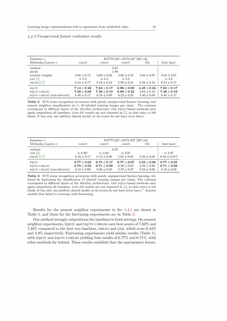
Datasets→ KITTI-227→SUN-227 [397 cls]Methods↓/Layers→ conv3 conv4 conv5 fc6 best layer
random 0.25pixels 1.80random weights 3.66± 0.12 3.60± 0.06 3.68± 0.25 4.04± 0.07 4.04± 0.07lsm [2] ≈ 4.9 ≈ 4.3 ≈ 4.3 - ≈ 4.9drlim [17] 6.44± 0.17 6.42± 0.23 5.80± 0.21 3.46± 0.10 6.44± 0.17
equiv 7.14± 0.22 7.62± 0.17 6.96± 0.09 4.48± 0.22 7.62± 0.17equiv+drlim 7.38± 0.08 7.48± 0.19 6.88± 0.22 3.84± 0.18 7.48± 0.19equiv+drlim (non-discrete) 6.46± 0.17 6.16± 0.09 6.22± 0.20 3.40± 0.08 6.46± 0.17
Table 2 SUN scene recognition accuracies with purely unsupervised feature learning, andnearest neighbor classification (k=1, 50 labeled training images per class) . The columnscorrespond to different layers of the AlexNet architecture. Our equiv-based methods onceagain outperform all baselines. (lsm fc6 results are not reported in [2], so that entry is leftblank. It has only one publicly shared model, so its scores do not have error bars.)
Datasets→ KITTI-227→SUN-227 [397 cls]Methods↓/Layers→ conv3 conv4 conv5 fc6 best layer
random 0.25lsm [2] ≈ 0.26∗ ≈ 1.04∗ ≈ 3.97 - ≈ 3.97drlim [17] 6.16± 0.17 6.12± 0.08 5.61± 0.05 3.32± 0.05 6.16± 0.017
equiv 6.77± 0.05 6.75± 0.17 6.77± 0.07 4.22± 0.06 6.77± 0.05equiv+drlim 6.70± 0.05 6.71± 0.08 6.36± 0.05 3.93± 0.06 6.71± 0.08equiv+drlim (non-discrete) 6.10± 0.08 6.00± 0.03 5.37± 0.07 3.53± 0.06 6.10± 0.08
Table 3 SUN scene recognition accuracies with purely unsupervised feature learning, fol-lowed by finetuning for classification (5 labeled training images per class). The columnscorrespond to different layers of the AlexNet architecture. Our equiv-based methods onceagain outperform all baselines. (lsm fc6 results are not reported in [2], so that entry is leftblank. It has only one publicly shared model, so its scores do not have error bars.) ∗ denotesmodels that failed to converge with finetuning.
Results for the nearest neighbor experiments in Sec 4.4.1 are shown inTable 2, and those for the finetuning experiments are in Table 3.
Our method strongly outperforms the baselines in both settings. On nearestneighbor experiments, equiv and equiv+drlim earn best scores of 7.62% and7.48% compared to the best two baselines, drlim and lsm, which score 6.44%and 4.9% respectively. Finetuning experiments yield similar results (Table 3),with equiv and equiv+drlim yielding best results of 6.77% and 6.71%, withother methods far behind. These results establish that the equivariance formu-
32 Dinesh Jayaraman, Kristen Grauman
lation more effectively exploits egomotion than the motion-regression approachof [2] for this data, and succeeds in learning generic image features.12
As expected, the pixel space baseline “pixels”, and the randomly initializedneural network “random weights” perform significantly worse than all othermethods on the nearest neighbor task in Table 2. The results also confirm theeffect of the inductive bias of the network architecture; the “random weights”baseline builds stronger representations than its input pixel space.
Finally, we also test the non-discrete variant of our approach, equiv+dr-lim (non-discrete). Recall from Sec 3.4, that this approach has an importantadvantage over equiv+drlim: it does not discretize the space of motions, soit may be able to more effectively exploit egomotion information. This varianttherefore allows us to evaluate whether this advantage is important empiricallyfor this dataset.
As shown in Table 2 and Table 3, equiv+drlim (non-discrete) is onceagain stronger than the baselines. However, it falls short of our standardequiv+drlim variant. This may be due to (i) the non-linear equivariancemap (cf. Sec 4.1) being too complex and thus weakening the constraint onthe learned feature space (cf. the discussion in Sec 3.2), (ii) the formulation ofEq (13) lacking the contrastive property of the loss of Eq (7); the feature spaceis held up from collapsing only by the contrastive term within drlim (Eq (9)),and (iii) the difficulty of learning a single effective function M in Eq (13), toencode feature transformations corresponding to all possible motions. Giventhe success of the discretized motion variant of our approach, we focus on itfor all subsequent experiments.
Interestingly, representations learned by all methods are most discrimina-tive at conv3 and conv4, and drop off at higher layers, especially fc6, wherefor nearest neighbor classification in Table 2, “random weights” performs bet-ter or on par with most methods. This suggests that model complexity ofthe networks may be too high in this setting (reproduced from [2]), given therelatively modest size of the KITTI dataset(≈20,500 video frames). Despitethis, equiv features perform reasonably well even at conv5 — in both Table 2and Table 3, equiv conv5 features are better than all baseline features at anylayer, suggesting that our egomotion-equivariance idea exploits unsupervisedKITTI data more efficiently than the baselines. In particular, the temporalcoherence objective of drlim appears to induce a loss of discriminativenessin feature layers close to fc6, the layer to which the loss is applied. drlim isbest at conv3, and while equiv+drlim performs similarly to equiv at lowerlayers, its performance significantly drops at higher layers compared to equiv.This is in keeping with our intuitions outlined in Sec 1; the drlim slow fea-ture analysis objective targets invariance, too much of which can lead to a lossof useful information for class discrimination. lsm too shows similar trends,falling off steadily in feature discriminativeness from conv3 to conv5, as seenin Table 2.
12 For fairness, Table 3 uses identical finetuning settings for all models (see Sec 4.4.2).Compared to its results in Table 3, the lsm baseline achieves higher scores on a relatedexperiment in [2], possibly due to differences in finetuning settings and train-test splits.
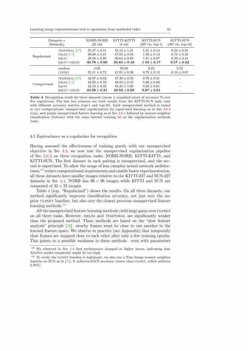
Learning image representations tied to egomotion from unlabeled video 33
Datasets→ NORB-NORB KITTI-KITTI KITTI-SUN KITTI-SUNMethods↓ [25 cls] [4 cls] [397 cls, top-1] [397 cls, top-10]
Regularized
temporal [37] 35.47± 0.51 45.12± 1.21 1.21± 0.14 8.24± 0.25drlim [17] 36.60± 0.41 47.04± 0.50 1.02± 0.12 6.78± 0.32equiv 38.48± 0.89 50.64± 0.88 1.31± 0.07 8.59± 0.16equiv+drlim 40.78± 0.60 50.84± 0.43 1.58± 0.17 9.57± 0.32
random 4.00 25.00 0.25 2.52clsnet 25.11± 0.72 41.81± 0.38 0.70± 0.12 6.10± 0.67
Unsupervised
temporal [37] 42.97± 0.62 47.39± 0.53 0.79± 0.01 -drlim [17] 42.83± 0.76 46.83± 0.45 0.86± 0.03 -equiv 42.18± 0.32 43.25± 1.00 0.56± 0.01 -equiv+drlim 44.08± 0.31 49.59± 0.66 0.87± 0.01 -
Table 4 Recognition result for three datasets (mean ± standard error) of accuracy % overfive repetitions. The last two columns are both results from the KITTI-SUN task, onlywith different accuracy metrics (top-1 and top-10). Each unsupervised method is testedin two configurations: unsupervised regularization for supervised learning as in Sec 3.6.2(top), and purely unsupervised feature learning as in Sec 3.6.1 followed by nearest neighborclassification (bottom) with the same labeled training set as the regularization methods(top).
4.5 Equivariance as a regularizer for recognition
Having assessed the effectiveness of training purely with our unsupervisedobjective in Sec 4.4, we now test the unsupervised regularization pipelineof Sec 3.6.2 on three recognition tasks: NORB-NORB, KITTI-KITTI, andKITTI-SUN. The first dataset in each pairing is unsupervised, and the sec-ond is supervised. To allow the usage of less complex neural network architec-tures,13 reduce computational requirements and enable faster experimentation,all these datasets have smaller images relative to the KITTI-227 and SUN-227datasets in Sec 4.4. NORB has 96 × 96 images while KITTI and SUN arecomposed of 32× 32 images.
Table 4 (top, “Regularized”) shows the results. On all three datasets, ourmethod significantly improves classification accuracy, not just over the no-prior clsnet baseline, but also over the closest previous unsupervised featurelearning methods.14
All the unsupervised feature learning methods yield large gains over clsneton all three tasks. However, drlim and temporal are significantly weakerthan the proposed method. Those methods are based on the “slow featureanalysis” principle [50]—nearby frames must be close to one another in thelearned feature space. We observe in practice (see Appendix) that temporallyclose frames are mapped close to each other after only a few training epochs.This points to a possible weakness in these methods—even with parameters
13 We observed in Sec 4.4 that performance dropped at higher layers, indicating thatAlexNet model complexity might be too high.14 To verify the clsnet baseline is legitimate, we also ran a Tiny Image nearest neighborbaseline on SUN as in [52]. It achieves 0.61% accuracy (worse than clsnet, which achieves0.70%).
34 Dinesh Jayaraman, Kristen Grauman
(temporal neighborhood size, regularization λ) cross-validated for recognition,the slowness prior is too weak to regularize feature learning effectively, sincestrengthening it causes loss of discriminative information. In contrast, ourmethod requires systematic feature space responses to egomotions, and offersa stronger prior.
The most exciting result is KITTI-SUN (the two rightmost columns in Ta-ble 4). The KITTI data itself is vastly more challenging than NORB due toits noisy ego-poses from inertial sensors, dynamic scenes with moving traffic,depth variations, occlusions, and objects that enter and exit the scene. Fur-thermore, the fact we can transfer equiv features learned without class labelson KITTI (street scenes from Karlsruhe, road-facing camera with fixed pitchand field of view) to be useful for a supervised task on the very different do-main of SUN (“in the wild” web images from 397 categories mostly unrelatedto streets) indicates the generality of our approach. Note that our method wasalso validated with larger images in this same KITTI-SUN setting in Sec 4.4.
Our best recognition accuracy of 1.58% on SUN is achieved with only 6labeled examples per class. It is ≈30% better than the nearest competingbaseline temporal and over 6 times better than chance. We also compute“Top-10” accuracy (last column) for SUN. This corresponds to the likelihoodof the true class being among the top-10 most likely classes according to theclassifier. Top-10 accuracy trends closely follow the standard top-1 accuracyresult, with equiv+drlim scoring 9.57% compared to 8.24% for the bestbaseline, temporal.
Comparison with purely unsupervised training: Finally, while the broad trendsobserved above are similar to those observed for the unsupervised training eval-uation in Sec 4.4, individual accuracies are not directly comparable with thosereported in Table 2 and 3, due to the differences in image sizes and networkarchitectures. To address this, we now repeat the experiments of Sec 4.4.1for these new datasets, performing nearest neighbor classification with purelyunsupervised features. Networks are trained with purely unsupervised losses.Features are then extracted and used in a nearest neighbor classifier (k = 1)using the target task training set (6, 4, and 6 labeled training images per classrespectively for NORB, KITTI, and SUN).
The results of these experiments, shown in Table 4 (bottom, “Unsuper-vised”), allow us to observe several trends. In general, we should expect thatregularization yields higher accuracies than purely unsupervised feature learn-ing followed by nearest neighbors — the regularization setting allows targetdomain and target task knowledge to influence the learning of the featuresthemselves. From Table 4, KITTI-SUN and KITTI-KITTI both follow theseexpected trends. Of these, KITTI-SUN results in particular are consistentlysignificantly poorer with purely unsupervised training, compared to regular-ization. We believe this is due to the large domain differences between KITTIand SUN, which mean that networks produced by purely unsupervised train-ing on KITTI may be less well-suited to processing SUN image inputs. This issupported by the fact that accuracies on KITTI-KITTI, where only the target
Learning image representations tied to egomotion from unlabeled video 35
dataset is changed and domains are matched, are only marginally better withregularization than with unsupervised training.
NORB-NORB accuracies are an exception in which purely unsupervisedtraining consistently performs slightly better than regularization. We believethat the toy neural network architecture employed in our NORB experiments(see Sec 4.1 and Fig 10) could prevent effective training, allowing a simplenearest neighbor classifier to be more effective. Finally, on both the “regu-larized” and “unsupervised” accuracies in Table 4, equiv+drlim featuresimprove significantly over equiv. This trend is thus consistent among exper-iments with small image datasets, but not observed in our experiments withlarger images in Sec 4.4. This suggests that the performance of equiv+drlimmay especially depend significantly on network architectures and/or featuredimensionality.
Varying training set sizes: We are especially interested in the impact of ourfeature learning idea when supervised training sets are relatively small. Thiscorresponds to handling categorization problems in the “long tail”, wheretraining samples are scarce and priors are most useful. However, we do con-tinue to see impact by our approach for larger training sets. For example, withN=20 samples for each of 397 classes on KITTI-SUN (7,940 total labeled train-ing images), equiv scores 3.66+/-0.08% accuracy vs. 1.66+/-0.18 for clsnet.Thus, our equivariance prior continues to boost recognition accuracy even atlarger training set sizes.
4.6 Next-best view selection for recognition
Finally, we show the results of a direct application of equivariant features to“next-best view selection” on NORB, as described in Sec 3.7 and illustrated inFig 8. Given one view of a NORB toy, the task is to tell a hypothetical robothow to move next, in order to best recognize the object, i.e, which neighboringview would best reduce object instance label prediction uncertainty.
To use the approach of Sec 3.7 for the baselines, we first compute equiv-ariance maps M ′
g for all methods as described in Sec 4.2. We set k = 25 forcomputing k-nearest neighbors, as per Sec 3.7.
Table 5 shows the results. On this task too, equiv features easily outper-form the baselines. Recall that our approach for this task is based on exploit-ing the predictability of feature responses to observer motions, i.e., featureequivariance. This result thus highlights the potential for many such novelapplications of our equivariant feature-learning formulation.
5 Conclusions and future work
Over the last decade, visual recognition methods have focused almost exclu-sively on learning from bags of images. We argue that such “disembodied”
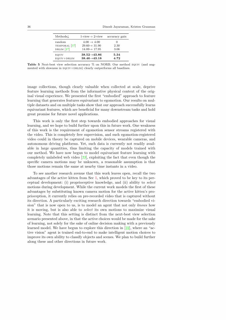
36 Dinesh Jayaraman, Kristen Grauman
Methods↓ 1-view→ 2-view accuracy gain
random 4.00 → 4.00 0temporal [37] 29.60→ 31.90 2.30drlim [17] 14.89→ 17.95 3.06
equiv 38.52→43.86 5.34equiv+drlim 38.46→43.18 4.72
Table 5 Next-best view selection accuracy % on NORB. Our method equiv (and aug-mented with slowness in equiv+drlim) clearly outperforms all baselines.
image collections, though clearly valuable when collected at scale, deprivefeature learning methods from the informative physical context of the orig-inal visual experience. We presented the first “embodied” approach to featurelearning that generates features equivariant to egomotion. Our results on mul-tiple datasets and on multiple tasks show that our approach successfully learnsequivariant features, which are beneficial for many downstream tasks and holdgreat promise for future novel applications.
This work is only the first step towards embodied approaches for visuallearning, and we hope to build further upon this in future work. One weaknessof this work is the requirement of egomotion sensor streams registered withthe video. This is completely free supervision, and such egomotion-registeredvideo could in theory be captured on mobile devices, wearable cameras, andautonomous driving platforms. Yet, such data is currently not readily avail-able in large quantities, thus limiting the capacity of models trained withour method. We have now begun to model equivariant feature learning withcompletely unlabeled web video [23], exploiting the fact that even though thespecific camera motions may be unknown, a reasonable assumption is thatthose motions remain the same at nearby time instants in a video.
To see another research avenue that this work leaves open, recall the twoadvantages of the active kitten from Sec 1, which proved to be key to its per-ceptual development: (i) proprioceptive knowledge, and (ii) ability to selectmotions during development. While the current work models the first of theseadvantages by substituting known camera motion for the active kitten’s pro-prioception, it currently relies on pre-recorded video that is captured withoutits direction. A particularly exciting research direction towards “embodied vi-sion” that is now open to us, is to model an agent that not only knows howit is moving, but is also able to select its own motions to maximize visuallearning. Note that this setting is distinct from the next-best view selectionscenario presented above, in that the active choices would be made for the sakeof learning, not solely for the sake of online decision making with a previouslylearned model. We have begun to explore this direction in [22], where an “ac-tive vision” agent is trained end-to-end to make intelligent motion choices toimprove its own ability to classify objects and scenes. We plan to build furtheralong these and other directions in future work.
Learning image representations tied to egomotion from unlabeled video 37
Acknowledgements This research is supported in part by ONR PECASE Award N00014-15-1-2291. We also thank Texas Advanced Computing Center for their generous support,Pulkit Agrawal for sharing models and code and for helpful discussions, Ruohan Gao forhelpful discussions, and our anonymous reviewers for their constructive suggestions.
References
1. Cuda-convnet. https://code.google.com/p/cuda-convnet/ 23, 242. Agrawal, P., Carreira, J., Malik, J.: Learning to see by moving. In: ICCV (2015) 7, 8,
21, 22, 23, 24, 29, 31, 323. Bojarski, M., Del Testa, D., Dworakowski, D., Firner, B., Flepp, B., Goyal, P., Jackel,
L.D., Monfort, M., Muller, U., Zhang, J., et al.: End to end learning for self-drivingcars. arXiv preprint arXiv:1604.07316 (2016) 7
4. Bromley, J., Bentz, J.W., Bottou, L., Guyon, I., LeCun, Y., Moore, C., Sackinger, E.,Shah, R.: Signature verification using a Siamese time delay neural network. IJPRAI(1993) 16
5. Cadieu, C.F., Olshausen, B.A.: Learning intermediate-level representations of form andmotion from natural movies. Neural computation (2012) 6, 11, 14, 22
6. Chen, C., Grauman, K.: Watching unlabeled videos helps learn new human actions fromvery few labeled snapshots. In: CVPR (2013) 6
7. Cohen, T.S., Welling, M.: Transformation Properties of Learned Visual Representations.ICLR (2015) 7
8. Dalal, N., Triggs, B.: Histograms of oriented gradients for human detection. In: CVPR(2005) 5, 6
9. Deng, J., Dong, W., Socher, R., Li, L.J., Li, K., Fei-Fei, L.: Imagenet: A large-scalehierarchical image database. In: Computer Vision and Pattern Recognition, 2009. CVPR2009. IEEE Conference on (2009) 27
10. Donahue, J., Jia, Y., Vinyals, O., Hoffman, J., Zhang, N., Tzeng, E., Darrell, T.: Decaf:A deep convolutional activation feature for generic visual recognition. In: ICML (2014)27
11. Dosovitskiy, A., Springenberg, J.T., Riedmiller, M., Brox, T.: Discriminative Unsuper-vised Feature Learning with Convolutional Neural Networks. NIPS (2014) 6
12. Gao, R., Jayaraman, D., Grauman, K.: Object-centric representation learning fromunlabeled videos. In: ACCV (2016) 6, 11, 14, 22
13. Geiger, A., Lenz, P., Stiller, C., Urtasun, R.: Vision meets Robotics: The KITTI Dataset.IJRR (2013) 5, 9, 22, 23
14. Geiger, A., Lenz, P., Urtasun, R.: Are we ready for autonomous driving? the KITTIvision benchmark suite. CVPR (2012) 5, 9, 22
15. Glorot, X., Bengio, Y.: Understanding the difficulty of training deep feedforward neuralnetworks. AISTATS (2010) 40
16. Goroshin, R., Bruna, J., Tompson, J., Eigen, D., LeCun, Y.: Unsupervised Learning ofSpatiotemporally Coherent Metrics. ICCV (2015) 5, 6, 11, 14, 22, 30
17. Hadsell, R., Chopra, S., LeCun, Y.: Dimensionality Reduction by Learning an InvariantMapping. CVPR (2006) 6, 13, 15, 16, 21, 22, 27, 31, 33, 36
18. Held, R., Hein, A.: Movement-produced stimulation in the development of visuallyguided behavior. Journal of comparative and physiological psychology (1963) 1, 2
19. Hinton, G.E., Krizhevsky, A., Wang, S.D.: Transforming Auto-Encoders. ICANN (2011)5, 6
20. Ioffe, S., Szegedy, C.: Batch normalization: Accelerating deep network training by re-ducing internal covariate shift. In: ICML (2015) 24
21. Jayaraman, D., Grauman, K.: Learning image representations tied to egomotion. In:ICCV (2015) 7
22. Jayaraman, D., Grauman, K.: Look-ahead before you leap: end-to-end active recognitionby forecasting the effect of motion (2016) 36
23. Jayaraman, D., Grauman, K.: Slow and steady feature analysis: higher order temporalcoherence in video. In: CVPR (2016) 36
38 Dinesh Jayaraman, Kristen Grauman
24. Jia, Y., Shelhamer, E., Donahue, J., Karayev, S., Long, J., Girshick, R., Guadarrama, S.,Darrell, T.: Caffe: Convolutional architecture for fast feature embedding. arXiv (2014)17, 40
25. Kivinen, J.J., Williams, C.K.: Transformation equivariant boltzmann machines. ICANN(2011) 5, 6, 11
26. Kornhauser, C.C.A.S.A., Xiao, J.: Deepdriving: Learning affordance for direct percep-tion in autonomous driving. ICCV (2015) 7
27. Krizhevsky, A., Sutskever, I., Hinton, G.E.: Imagenet classification with deep convolu-tional neural networks. In: NIPS (2012) 27, 29
28. Kulkarni, T.D., Whitney, W., Kohli, P., Tenenbaum, J.B.: Deep convolutional inversegraphics network. NIPS (2015) 5, 6
29. LeCun, Y., Huang, F.J., Bottou, L.: Learning methods for generic object recognitionwith invariance to pose and lighting. CVPR (2004) 22, 23
30. Lenc, K., Vedaldi, A.: Understanding image representations by measuring their equiv-ariance and equivalence. CVPR (2015) 5, 6, 11, 26
31. Levine, S., Finn, C., Darrell, T., Abbeel, P.: End-to-end training of deep visuomotorpolicies. arXiv preprint arXiv:1504.00702 (2015) 7
32. Li, Y., Fathi, A., Rehg, J.M.: Learning to predict gaze in egocentric video. In: ICCV(2013) 7
33. Lies, J.P., Hafner, R.M., Bethge, M.: Slowness and sparseness have diverging effects oncomplex cell learning. PLoS computational biology (2014) 6, 11, 14, 22
34. Lowe, D.: Object recognition from local scale-invariant features. In: ICCV (1999) 5, 635. Memisevic, R.: Learning to relate images. PAMI (2013) 736. Michalski, V., Memisevic, R., Konda, K.: Modeling Deep Temporal Dependencies with
Recurrent Grammar Cells. NIPS (2014) 5, 737. Mobahi, H., Collobert, R., Weston, J.: Deep Learning from Temporal Coherence in
Video. ICML (2009) 5, 6, 11, 14, 16, 21, 22, 27, 33, 3638. Nakamura, T., Asada, M.: Motion sketch: Acquisition of visual motion guided behaviors.
IJCAI (1995) 739. Ranzato, M., Szlam, A., Bruna, J., Mathieu, M., Collobert, R., Chopra, S.: Video (lan-
guage) modeling: a baseline for generative models of natural videos. arXiv (2014) 5,7
40. Ren, X., Gu, C.: Figure-Ground Segmentation Improves Handled Object Recognitionin Egocentric Video. In: CVPR (2010) 7
41. Schmidt, U., Roth, S.: Learning rotation-aware features: From invariant priors to equiv-ariant descriptors. CVPR (2012) 5, 6, 11
42. Simard, P., LeCun, Y., Denker, J., Victorri, B.: Transformation Invariance in PatternRecognition - Tangent distance and Tangent propagation (1998) 6
43. Simard, P.Y., Steinkraus, D., Platt, J.C.: Best practices for convolutional neural net-works applied to visual document analysis. ICDAR (2003) 6
44. Sohn, K., Lee, H.: Learning invariant representations with local transformations. ICML(2012) 6
45. Tulsiani, S., Carreira, J., Malik, J.: Pose induction for novel object categories. In: ICCV(2015) 6
46. Tuytelaars, T., Mikolajczyk, K.: Local invariant feature detectors: a survey. Foundationsand trends in computer graphics and vision 3(3), 177–280 (2008) 5, 6
47. Vincent, P., Larochelle, H., Bengio, Y., Manzagol, P.A.: Extracting and composingrobust features with denoising autoencoders. ICML (2008) 6
48. Wang, X., Gupta, A.: Unsupervised learning of visual representations using videos. In:CVPR (2015) 5, 6, 11, 14, 30
49. Watter, M., Springenberg, J., Boedecker, J., Riedmiller, M.: Embed to control: A locallylinear latent dynamics model for control from raw images. In: NIPS (2015) 7
50. Wiskott, L., Sejnowski, T.J.: Slow feature analysis: unsupervised learning of invariances.Neural computation (2002) 6, 33
51. Wu, Z., Song, S., Khosla, A., Tang, X., Xiao, J.: 3d shapenets for 2.5 d object recognitionand next-best-view prediction. CVPR (2015) 20
52. Xiao, J., Hays, J., Ehinger, K.A., Oliva, A., Torralba, A.: Sun database: Large-scalescene recognition from abbey to zoo. CVPR (2010) 5, 23, 24, 33
Learning image representations tied to egomotion from unlabeled video 39
53. Xu, C., Liu, J., Kuipers, B.: Moving object segmentation using motor signals. ECCV(2012) 7
54. Yamada, K., Sugano, Y., Okabe, T., Sato, Y., Sugimoto, A., Hiraki, K.: Attentionprediction in egocentric video using motion and visual saliency. PSIVT (2012) 7
55. Zou, W., Zhu, S., Yu, K., Ng, A.Y.: Deep learning of invariant features via simulatedfixations in video. NIPS (2012) 6, 11, 14, 22
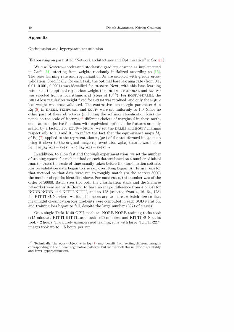
40 Dinesh Jayaraman, Kristen Grauman
Appendix
Optimization and hyperparameter selection
(Elaborating on para titled “Network architectures and Optimization” in Sec 4.1)
We use Nesterov-accelerated stochastic gradient descent as implementedin Caffe [24], starting from weights randomly initialized according to [15].The base learning rate and regularization λs are selected with greedy cross-validation. Specifically, for each task, the optimal base learning rate (from 0.1,0.01, 0.001, 0.0001) was identified for clsnet. Next, with this base learningrate fixed, the optimal regularizer weight (for drlim, temporal and equiv)was selected from a logarithmic grid (steps of 100.5). For equiv+drlim, thedrlim loss regularizer weight fixed for drlim was retained, and only the equivloss weight was cross-validated. The contrastive loss margin parameter δ inEq (8) in drlim, temporal and equiv were set uniformly to 1.0. Since noother part of these objectives (including the softmax classification loss) de-pends on the scale of features,15 different choices of margins δ in these meth-ods lead to objective functions with equivalent optima - the features are onlyscaled by a factor. For equiv+drlim, we set the drlim and equiv marginsrespectively to 1.0 and 0.1 to reflect the fact that the equivariance maps Mg
of Eq (7) applied to the representation zθ(gx) of the transformed image mustbring it closer to the original image representation zθ(x) than it was beforei.e., ‖Mgzθ(gx)− zθ(x)‖2 < ‖zθ(gx)− zθ(x)‖2.
In addition, to allow fast and thorough experimentation, we set the numberof training epochs for each method on each dataset based on a number of initialruns to assess the scale of time usually taken before the classification softmaxloss on validation data began to rise i.e., overfitting began. All future runs forthat method on that data were run to roughly match (to the nearest 5000)the number of epochs identified above. For most cases, this number was of theorder of 50000. Batch sizes (for both the classification stack and the Siamesenetworks) were set to 16 (found to have no major difference from 4 or 64) forNORB-NORB and KITTI-KITTI, and to 128 (selected from 4, 16, 64, 128)for KITTI-SUN, where we found it necessary to increase batch size so thatmeaningful classification loss gradients were computed in each SGD iteration,and training loss began to fall, despite the large number (397) of classes.
On a single Tesla K-40 GPU machine, NORB-NORB training tasks took≈15 minutes, KITTI-KITTI tasks took ≈30 minutes, and KITTI-SUN taskstook ≈2 hours. The purely unsupervised training runs with large “KITTI-227”images took up to 15 hours per run.
15 Technically, the equiv objective in Eq (7) may benefit from setting different marginscorresponding to the different egomotion patterns, but we overlook this in favor of scalabilityand fewer hyperparameters.
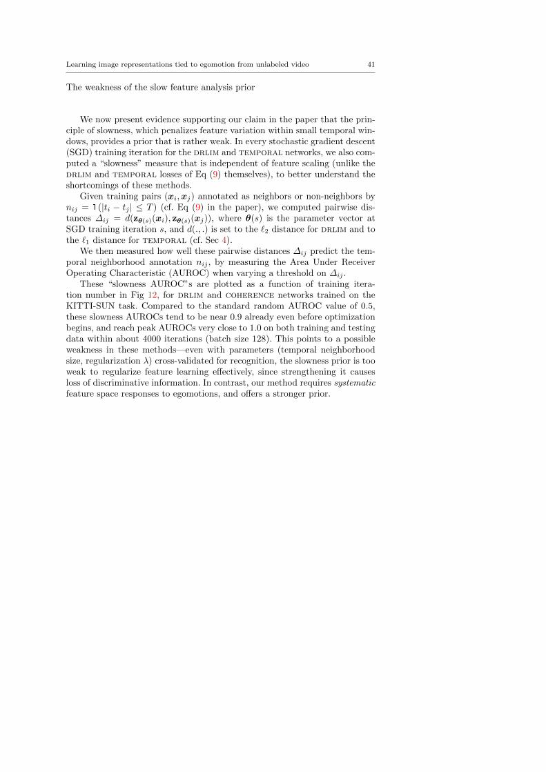
Learning image representations tied to egomotion from unlabeled video 41
The weakness of the slow feature analysis prior
We now present evidence supporting our claim in the paper that the prin-ciple of slowness, which penalizes feature variation within small temporal win-dows, provides a prior that is rather weak. In every stochastic gradient descent(SGD) training iteration for the drlim and temporal networks, we also com-puted a “slowness” measure that is independent of feature scaling (unlike thedrlim and temporal losses of Eq (9) themselves), to better understand theshortcomings of these methods.
Given training pairs (xi,xj) annotated as neighbors or non-neighbors bynij = 1(|ti − tj | ≤ T ) (cf. Eq (9) in the paper), we computed pairwise dis-tances ∆ij = d(zθ(s)(xi), zθ(s)(xj)), where θ(s) is the parameter vector atSGD training iteration s, and d(., .) is set to the `2 distance for drlim and tothe `1 distance for temporal (cf. Sec 4).
We then measured how well these pairwise distances ∆ij predict the tem-poral neighborhood annotation nij , by measuring the Area Under ReceiverOperating Characteristic (AUROC) when varying a threshold on ∆ij .
These “slowness AUROC”s are plotted as a function of training itera-tion number in Fig 12, for drlim and coherence networks trained on theKITTI-SUN task. Compared to the standard random AUROC value of 0.5,these slowness AUROCs tend to be near 0.9 already even before optimizationbegins, and reach peak AUROCs very close to 1.0 on both training and testingdata within about 4000 iterations (batch size 128). This points to a possibleweakness in these methods—even with parameters (temporal neighborhoodsize, regularization λ) cross-validated for recognition, the slowness prior is tooweak to regularize feature learning effectively, since strengthening it causesloss of discriminative information. In contrast, our method requires systematicfeature space responses to egomotions, and offers a stronger prior.
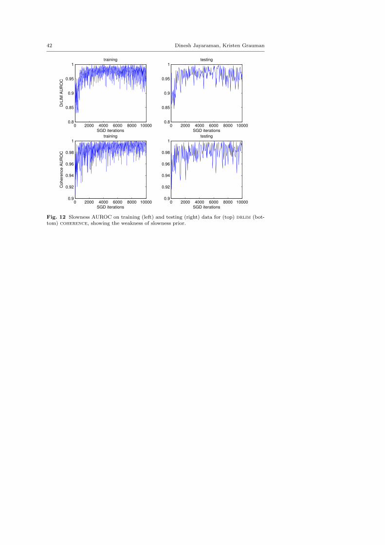
42 Dinesh Jayaraman, Kristen Grauman
0 2000 4000 6000 8000 100000.8
0.85
0.9
0.95
1training
SGD iterations
DrL
IM A
UR
OC
0 2000 4000 6000 8000 100000.8
0.85
0.9
0.95
1testing
SGD iterations
0 2000 4000 6000 8000 100000.9
0.92
0.94
0.96
0.98
1training
SGD iterations
Cohere
nce A
UR
OC
0 2000 4000 6000 8000 100000.9
0.92
0.94
0.96
0.98
1testing
SGD iterations
Fig. 12 Slowness AUROC on training (left) and testing (right) data for (top) drlim (bot-tom) coherence, showing the weakness of slowness prior.