learning linear dependency trees from multivariate time-series data

8/14/2019 Learning Linear Dependency Trees From Multivariate Time-Series Data

http://slidepdf.com/reader/full/learning-linear-dependency-trees-from-multivariate-time-series-data 1/10

Learning Linear Dependency Trees from Multivariate Time-series Data

Jarkko Tikka and Jaakko Hollm enHelsinki University of Technology

Laboratory of Computer and Information ScienceP.O. Box 5400, FIN-02015 HUT, Finland

[email protected]., Jaakko.Hollmen@hut.

Abstract

Representing interactions between variables in largedata sets in an understandable way is usually important and hard task. This article presents a methodology howa linear dependency structure between variables can beconstructed from multivariate data. The dependencies be-tween the variables are specied by multiple linear regres-sion models. A sparse regression algorithm and bootstrapbased resampling are used in the estimation of models and in construction of a belief graph. The belief graph high-lights the most important mutual dependencies between thevariables. Thresholding and graph operations may be applied to the belief graph to obtain a nal dependency struc-ture, which is a tree or a forest. In the experimental sectionresults of the proposed method using real-world data set

were realistic and convincing.

1. Introduction

Large data sets are available from many differentsources, for example from industrial processes, economy,mobile communications network, and environment. Deeperunderstanding of the underlying process can be achieved byexploring or analyzing the data. Economical or ecologicalbenets are a great motivation for the data analysis.

In this study, dependencies between the variables in dataset are analyzed. The purpose is to estimate multiple linearregression models and learn a linear dependency tree or for-est of the variables. The dependency structure clearly showshow a change in a value of one variable induces changes invalues of other variables. This might be useful informationin many cases, for instance, if values of some variable can-not be controlled directly.

The multiple linear regression models have a couple of advantages. The dependencies in linear models are easy tointerpret. In addition, processes may be inherently linear or

Data

1 2

DependencyStructure

5

DependencyGraph

43

PreprocessingEstimation of

via the bootstraplinear models

Figure 1. The ow chart of the proposedmethod.

over short ranges many processes can be approximated by alinear model.

A ow chart of the methodology proposed in this studyis presented in Figure 1. The method consists of ve phases.First, there should be some multivariate data available. Thedata do not necessarily have to be time-series data, althoughtime-series data is used as an example in this study.

The second phase deals with the preprocessing of data.Some operations have to be usually performed on measure-ments before they can be analyzed mathematically. Somemeasurements may be missing or measurements can benoisy.

In the third phase, as many multiple linear regressionmodels as there are variables in the data are estimated. Eachvariable is a dependent variable in turn and the rest of thevariables are possible independent variables. The most sig-nicant independent variables for each model are selectedusing the bootstrap and a sparse regression algorithm. Therelative weights of the regression coefcients are computedfrom the bootstrap replications. The relative weight of theregression coefcient measures a belief that the correspond-ing independent variable belongs to the estimated linearmodel.

In the fourth phase, a belief graph is constructed from therelative weights of the regression coefcients. The belief graph represents the strength of the dependencies betweenthe variables. In the belief graph there are as many nodesas there are variables in the data. The relative weights de-ne arcs of the belief graph. A predened threshold valueand a moralizing operation are applied to the belief graph



resulting a moral graph or a nal dependency graph.Finally, a dependency structure of the variables is calcu-

lated from the dependency graph. A set of variables, whichforms a multiple linear regression model, belongs to a samemaximal clique. However, the formulation of nal depen-dency structure is restricted such that the dependencies can-not form circles in a nal structure i.e. the variable cannotbe dependent on itself through the other variables. Thus, thenal dependency structure is a tree or a forest.

The rest of the article is organized as follows. In Sec-tion 2 a few other similar studies are briey described. Themultiple linear regression model and sparse regression al-gorithms are introduced in the beginning of Section 3, fol-lowed by the bootstrap and the computation of the relativeweights of the regression coefcients. The construction of linear dependency tree or forest is proposed in Section 4.The proposed method is applied to real-world data set. Thedescription of data and the results of experiments are shown

in Section 5. The experiments mainly serve an illustrativeexample of the proposed methodology. Conclusion and -nal remarks are in Section 6.

2 Related work

To our knowledge, novelty of this work is in the sparseconstruction of linear models and the application of thebootstrap. Several studies about dependencies between thevariables in multivariate data are accomplished, for example[3], [13], [11], [16], and [20].

Dependency trees are also used in [3]. A method which

approximates optimally a d-dimensional probability distri-bution of the d variables is shown. Each variable can onlybe dependent on at most one variable in that model, whenin this study one variable can be dependent on several vari-ables.

Belief networks are discussed in [13]. The belief net-work induces a conditional probability distribution over itsvariables. The belief networks are directed and acyclic. De-pendency networks which can be cyclic are presented in[11]. In both belief and dependency networks the variablesare conditioned upon its parent variables. The directed de-pendency means that changes in the parent has effect on thechild. The undirected dependency means that changes areinduced into the both directions. In this study, continuousvariables are only modeled, whereas the belief and the de-pendency network can be used with discrete variables.

Independent variable group analysis (IVGA) is proposedin [16]. In that approach the variables are clustered. Thevariables in one cluster are dependent on each other butthey are independent on the variables which belong to otherclusters. In IVGA, the dependencies between the groups orclusters are ignored and the dependencies in each group canbe modeled in different ways.

Structural equation modeling (SEM) [20] is anothertechnique to investigate relationships between the variables.SEM provides a methodology to test a plausibility of hy-pothesized models. The predened dependencies betweenthe variables are investigated using the SEM, when the de-pendencies are learned from the data using the method pro-posed in this study. Structural Equation models can consistof both observed and latent variables. The latent variablescan be extracted from the observed ones using for examplethe factor analysis. Observed variables are only modeled inthis study.

3 Methods

3.1 Multiple linear regression

The dependencies between the variables are modeled us-ing the multiple linear regression. The model is

yt = β 1 x t, 1 + β 2 x t, 2 + . . . + β k x t,k + ǫt , (1)

where yt is the dependent variable, x t,i , i = 1 , . . . , k arethe independent variables, β i , i = 1 , . . . , k are the corre-sponding regression coefcients, and ǫt is normally dis-tributed random noise with zero mean and unknown vari-ance ǫt ∼ N (0, σ 2 ). The index t = 1 , . . . , N representsthe t th observation of the variables y and x i and N is thesample size.

Equation (1) can also be written in matrix form as fol-lows

y = Xβ + ǫ. (2)Here we assume that the variables are normalized to zeromean and thus, there is no need for a constant term in mod-els (1) and (2).

The ordinary least squares (OLS) solution is

bOLS = ( X T X )− 1 X T y (3)

where bOLS = [b1 , . . . , bk ] is the best linear unbiased esti-mate of the regression coefcients.

3.2 Linear sparse regression

The usual situation is that the available data are(x 1 , . . . , x k , y ) and the linear regression model should beestimated. The OLS estimates are calculated using all theindependent variables. However, the OLS estimates maynot always be satisfactory. The number of possible inde-pendent variables may be large and there are likely non-informative variables among them.

The OLS estimates have a low bias but a large variance.The large variance impairs the prediction accuracy. The pre-diction accuracy can sometimes be improved by shrinking



some regression coefcients toward zero, although at thesame time the bias increases [4]. The models with too manyindependent variables are also difcult to interpret. Now,the objective is to nd a smaller subset of independent vari-ables that have the strongest effect in the regression model.

In the subset selection regression only a subset of theindependent variables are included to the model, but it isan inefcient approach if the number of independent vari-ables is large. The subset selection is not robust becausesmall changes in the data can result in very different mod-els. More stable result can be achieved using the nonnega-tive garrote [2]. The garrote also eliminates some variablesand shrinks other coefcients by some positive values.

Ridge regression [12] and lasso [22] algorithms producea sparse solution or at least shrink estimates of the regres-sion coefcients toward zero. Both algorithms minimize apenalized residual sum of squares

argminβ

|| y − Xβ || 2 + λk

i =1

|β i |γ , (4)

where γ = 2 in ridge regression and γ = 1 in lasso. Thetuning parameter λ controls the amount of shrinkage that isapplied to the coefcients. The problem in Equation (4) canbe represented equivalently as a constrained optimizationproblem. In that approach the residual sum of squares || y −Xb || 2 is minimized subject to

k

i =1

|β i |γ ≤ τ, (5)

where γ is the same as in Equation (4) and the constantτ controls the amount of the shrinkage. The parameters λin Equation (4) and τ in Equation (5) are related to eachother by a one-to-one mapping [10]. A large value of λcorresponds to a small value of τ .

The ridge regression solution is easy to calculate, be-cause the penalty term is continuously differentiable. Thesolution is

bRR = ( X T X + λ I )− 1 X T y , (6)

where I is an identity matrix, but it does not necessarilyset any coefcients exactly to zero. Thus, the solution isstill hard to interpret if the number of independent variablesk is large. The lasso algorithm sets some coefcients tozero with a proper τ , but nding the lasso solution is morecomplicated due to absolute values in the penalty term. Aquadratic programming algorithm has to be used to computethe solution. Also, the value of τ or λ which controls theshrinkage is strongly dependent on data. Therefore, seek-ing such a value may be difcult in many cases. The data-based techniques for estimation of the tuning parameter τ are presented in [22].

x i 1ˆ

y 0ˆ

y 1

ˆ

y 2

y 3

y 2

y 1

x i 2

x i 3

u 1

u 2

u 3

Figure 2. The progress of the LARS algorithm.The gure is reproduced from the originalLARS article by Efron et al. [7].

The lasso algorithm is not applicable if the number of

possible independent variables is large. Forward stagewiselinear regression (FSLR) can be used instead of lasso inthat case [10]. FSLR approximates the effect of the lassopenalty γ = 1 in Equation (4). New independent variablesare added sequentially to the model in FSLR. Two constantsδ and M have to be set before iterations. The regressioncoefcient that diminish most the current residual sum of squares, is adjusted by amount of δ at each successive iter-ation. The value of δ should be small and M should be arelatively large number of iterations.

All the estimates of coefcients bi , i = 1 , . . . , k are set tozero in the beginning. Many of the estimates bi are possibly

still zero after M iterations. It means that correspondingindependent variables are not yet added to the regressionmodel. The solution after the M iterations is almost similarthan the lasso solution with some λ . They are even identicalin some cases [10].

The preceding methods such as ridge regression, lasso,and FSLR are introduced as the historical precursors of theLeast Angle Regression (LARS) model selection algorithm.We are mainly interested in the methods producing sparsemodels. Thus, lasso and FSLR could be applied, but theyhave deciencies compared to the LARS algorithm. Theparameters λ or τ in lasso and δ and M in FSLR have tobe predened, whereas LARS is completely parameter freeand it is also computationally more efcient than lasso orFSLR. However, all the three methods produce nearly samesolutions. Only LARS algorithm is applied to selection of the most signicant independent variables in this study.

In Figure 2 the progress of the LARS algorithm is vi-sualized. All the variables are scaled to have zero meanand unit variance. One independent variable is added to themodel in each step. First, all regression coefcients are setto zero. Then, the most correlated independent variable x i 1

with y is found. The largest possible step in the direction



of u 1 is taken until some other variable x i 2 is as correlatedwith the current residuals as x i 1 . That is the point y 1 . Atthis point LARS differs from traditional Forward Selection,which would proceed to the point y 1 , but the next step inLARS is taken in a direction u 2 equiangular between x i 1

and x i 2 . LARS proceeds in this direction until a third vari-able x i 3 is as correlated with the current residuals as x i 1

and x i 2 . Next step is taken in a direction u 3 equiangularbetween x i 1 , x i 2 , and x i 3 until a fourth variable can beadded to the model. This procedure is continued as longas there are still independent variables left. So, k steps areneeded for the full set of solutions i.e. the result is k differ-ent multiple linear regression models. In Figure 2 y i repre-sent the corresponding OLS estimates from kth step. LARSestimates y k approach but never reach OLS estimates y k ,except at the last step the LARS and OLS estimates areequivalent. The mathematical details of LARS algorithmare presented in [7].

The problem is to nd the best solution from all the kpossibilities which LARS returns i.e. a proper number of independent variables. This selection can be done accord-ing to the minimum description length (MDL) informationcriterion [9]. The variance σ2 of ǫt is assumed to be un-known, thus, the MDL criterion is written in context of thelinear regression, as presented in [9],

MDL (k) =N 2

log || y − y || 2 +k2

log N. (7)

y is the dependent variable, y is the estimate of the depen-dent variable, N is the sample size and k is the number

of added independent variables. The value of Equation (7)is calculated for all the solutions. The selected regressionmodel minimizes Equation (7).

The Mallows C p criterion [18], [19] is a common crite-rion in subset selection. However, C p is not used, because itcan select submodels of too high dimensionality [1]. A re-view of several other information criteria can be found from[21].

3.3 Bootstrap

The bootstrap is a statistical resampling method and itwas introduced by Efron in [6]. The idea of bootstrap is touse sample data to estimate some statistics of the data. Noassumptions are made about the forms of probability distri-butions in the bootstrap procedure. The statistic of interestand its distribution are computed by resampling the originaldata with replacement.

Bootstrapping a regression model can be done in twodifferent ways. The methods are bootstrapping residualsand bootstrapping pairs [8]. The independent variables(x 1 , . . . , x k ) are treated as xed quantities in the bootstrap-ping residuals approach. That assumption is strong and it

can fail even if Equation (1) for the regression model is cor-rect. In the bootstrapping pairs approach weaker assump-tions about validity of Equation (1) are made.

In the bootstrapping pairs, F is assumed to bean empirical distribution of the observed data vectors(x t, 1 , . . . , x t,k , yt ), where t = 1 , . . . , N . F puts prob-ability mass of 1/N on each vector (x t, 1 , . . . , x t,k , yt ).A bootstrap sample is now a random sample of size N drawn with replacement from the population of N vectors(x t, 1 , . . . , x t,k , yt ).

B independent bootstrap samples (X ∗ i , y ∗ i ), i =1, . . . , B of the size N are drawn from the distribution F .The bootstrap replications b∗ i of the estimates b are com-puted using the LARS algorithm and the MDL informationcriterion. The statistic of interest or some other features of the parameters b can be calculated from these B bootstrapreplications.

3.4 Computation of relative weights of regressionmodel

In this study, relative weights of the coefcients of mul-tiple linear regression model are computed. The relativeweights are calculated from the bootstrap replications asfollows

w =1B

B

i =1

|b∗ i |1 T |b∗ i |

. (8)

B is the number of bootstrap replications and b∗ i is the ithbootstrap replication of coefcients b. The absolute values

are taken over all the components of vector b∗ i

. There isa sum of the absolute values of coefcients in the denomi-nator. 1 is a vector of ones and the length of the vector isthe same as the length of the vector b∗ i . All the compo-nents of vector |b∗ i | are divided by the previous sum. Theseoperations are done for every bootstrap replication and thescaled bootstrap replications are added together. This sumis divided by the number of bootstrap samples B . The re-sult is a vector w , which includes the relative weights of thecoefcients b.

There is a relative weight wi for the each possible inde-pendent variable x i , i = 1 , . . . , k in the vector w . The valueof each w

iis within the range w

i∈ [0, 1] and

iw

i= 1 .

The relative weight of the independent variable is a measureof the belief that the independent variable belongs to the es-timated linear model. The independent variable can be re-

jected from the estimated model if the value of wi is zeroor under a predened threshold value. The most signi-cant independent variables have the largest relative weights.In this study the variables are scaled to have unit variance,therefore, the regression coefcients are comparable to eachother and their absolute values can be used as a measure of signicance.



The vector of relative weights can also be regarded as adiscrete probability distribution. From the probability dis-tribution it can be seen which independent variables arelikely to be included to the nal linear sparse regressionmodel.

4 Learning a linear dependency structure

4.1 Constructing a belief graph

Let us assume now that there are data D available, whichhave k +1 variables and N measurements for each variable.The objective is to nd multiple linear regression modelsamong the variables. Each variable is the dependent vari-able in turn and the rest of the variables are the possibleindependent variables. So, the following models have to beestimated.

x 1 = b1

2x 2 + b1

3x 3 + . . . + b1

kx k + b1

k +1x k +1

x 2 = b21 x 1 + b2

3 x 3 + . . . + b2k x k + b2

k +1 x k +1

...

x j = bj1 x 1 + . . . + bj

j − 1 x j − 1 + bjj +1 x j +1 + . . .

bjk +1 x k +1

...

x k = bk1 x 1 + bk

2 x 2 + . . . + bkk − 1 x k − 1 + bk

k +1 x k +1

x k +1 = bk +11 x 1 + bk +1

2 x 2 + . . . + bk +1k − 1 x k − 1 + bk +1

k x k

The relative weights of the regression coefcients are com-

puted for all the above k + 1 linear models as it is describedin Sections 3.2-3.4. A belief graph Gb is constructed fromthese k + 1 vectors of the relative weights.

Each variable of data D is presented as a node in the be-lief graph Gb . The weighted arcs between the nodes are ob-tained from the nonzero relative weights. Thus, the weightsof arcs measure the strength of the belief that there existsa linear dependency between the corresponding two vari-ables. The directions of dependencies are from the inde-pendent variable to the dependent variable.

The dependencies or the number of arcs in the belief graph can be reduced by setting some threshold value λ forthe relative weights. The relative weight is set to zero if itis below the threshold and the rest of the relative weightsare set to unity. This means that remaining dependenciesare treated as equally important thereafter. The belief graphGb becomes unweighted directed graph Gd after using thethreshold λ . However, some dependencies may be bidirec-tional. The value of threshold is not estimated according tosome dened principle. A suitable value for λ is decidedby exploring the values of relative weights. The purpose isto nd such value for λ that minor changes in λ would notcause major changes in the graph Gd .

The direct use of the full information in the belief graphwill be studied further.

4.2 Constructing a moral graph

The following idea of constructing an undirected and amoral graph from the belief graph is adapted from [13]. LetV i , i = 1 , . . . , k stand for a node or a variable in the graphs.The directions of dependencies can be discarded from Gd

and the result is an unweighted undirected graph Gu . Itcan be assumed now that two variables V i and V j belongpotentially to the same linear model if they are connectedby an arc in Gu . We mean that the variables belong possiblyto the same set of variables which forms one linear sparseregression model. That is, the roles of the variables V i andV j either as independent variable or dependent variable arenot specied yet.

Let us assume that a variable x j 3 is the actual dependentvariable. A possible regression model is x j 3 = β j 1 x j 1 +β j 2 x j 2 + φ, where φ is a function of the other independentvariables and noise. When variables x j 1 and x j 2 are consid-ered as the dependent variables, it is possible that the depen-dency with the variable x j 3 is found, but the dependenciesbetween x j 1 and x j 2 are ignored in both cases. However,all three variables x j 1 , x j 2 , and x j 3 belong potentially tothe same linear model. An arc can be added to connect thecorresponding nodes in Gu . The added arc is called a moralarc. A moral graph Gm is obtained when all moral arcshave been added to Gu . The moral arcs are added to Gu

according to the following procedure.

• Create a directed graph G ′

u from Gu . The directions of dependencies are set to graph G ′

u such that there do notexist cycles. For each node V i , nd its parents P V i inG ′

u . Connect each pair of nodes in P V i by adding undi-rected arcs between the corresponding nodes in Gu .

In this study, the graph G ′

u is created from Gu such thatthe parent V i has a smaller index than the child V j i.e. i < jin G ′

u . This restriction conrms that the relationships canbe interpreted correctly and the number of added moral arcsis reasonable. The parent and child relationships can be de-ned differently to G ′

u as above and it likely results in a dis-similar moral graph and a nal dependency structure. Thenal dependency structure can be constructed as well fromGu as from Gm . Basically, sparser models are obtainedfrom Gu , but the moral arc addition can give additional use-ful information in some cases.

4.3 Constructing nal linear models

The objective is to nd multiple linear regression mod-els among the variables in the data D . The linear models or



the sets of variables are sought from the unweighted undi-rected graph Gu or from the moral graph Gm . The vari-ables, which are interpreted to belong to the same model,are parts of the same maximal clique. A subgraph of Gu orGm is called a clique if the subgraph is complete and max-imal. A subgraph is complete, if every pair of nodes in thesubgraph is connected by an arc. The clique is maximal, if it is not a subgraph of the larger complete subgraph [13].

An algorithm, which can be used to generate all maximalcliques from an arbitrary undirected graph, is presented indetail in [15]. A short description of the algorithm is givenin the next two paragraphs.

Let C n stand for a list of all cliques which include nnodes. The algorithm starts by forming all 2-cliques. Allpairs of nodes which are connected by an arc are 2-cliques.There exists 3-clique if two 2-cliques have one node incommon and two sole nodes are connected. For example,if there are cliques {V 1 , V 2 }, {V 1 , V 3 } and {V 2 , V 3 } in the

graph, then there exists 3-clique {V 1 , V 2 , V 3 }. All 3-cliquesare collected to the list C 3 .

All (n + 1) -cliques can be constructed from the list C n .Two n -cliques c1

n and c2n , which have already (n − 1) nodes

in common, are tested if they could form a new (n + 1) -clique cn +1 . There has to exist n -clique c3

n , which has (n −2) nodes in common with cliques c1

n and c2n , in the list C n .

Additionally, (n− 1)th node of c3n has to be equivalent to n th

node of c1n and n th node of c3

n has to be equivalent to n thnode of c2

n , then there is (n + 1) -clique cn +1 in the graph.For example, if there exist cliques c1

4 = {V 1 , V 2 , V 3 , V 4 },c2

4 = {V 1 , V 2 , V 3 , V 5 } and c34 = {V 1 , V 2 , V 4 , V 5 }, then there

exist 5-clique c5 = {V 1 , V 2 , V 3 , V 4 , V 5 } in the graph. Thisprocedure is repeated as long as new cliques can be con-structed. All lists C i , i = 1 , . . . , n max are tested in theend, that any n -clique is not a subclique of (n + m)-clique,m > 0. If there exist subcliques they can be eliminated. Inthe end, the dependent variable in all the cliques is selectedsuch that the coefcient of determination is maximized.

The problem to nd all maximal cliques is known to beNP -hard [14]. This means that the computational time for asolution is nondeterministic and the number of cliques canincrease exponentially. Several other algorithms for solv-ing the clique problem are introduced and analyzed in [14].Computationally, the task is feasible, if the number of vari-ables in the data D is not large. The number of variablescan be a few hundred. The number of arcs in the graph alsoaffects on the computational efciency.

The number of found complete and maximal cliques canbe large, but there are additional criteria how nal cliquesare selected. Firstly, two cliques can have only one variableor node in common. Secondly, the common variable can-not be a dependent variable in both cliques. Finally, cyclesare not allowed in the dependency structure. Therefore, thedependency structure is a dependency tree or a forest under

these restrictions. The independent variables are the parentsof the dependent variable in the nal dependency structure.The construction of the dependency structure starts from thelinear model which has the highest coefcient of determi-nation. After that, the linear models are added such that thecoefcients of determination are as good as possible and theprevious restrictions are not violated.

5 Experiments

5.1 Data

A real-world data set which is used in this study is calledthe System data. The System data consist of nine measure-ments from a single computer which is connected to a net-work. The computer is used for example to edit programsor publications and to calculate computationally intensivetasks [23].

Four of the variables describe the network trafc. Rest of the variables are measurements from the central processingunit (CPU). All the variables are in relative measures in thedata set. The variables are 1. blks/s (read blocks persecond (network)), 2. wblks/s (written blocks per second(network)), 3. usr (time spent in user processes (CPU)), 4.sys (time spent in system processes (CPU)), 5. intr (timespent handling interrupts (CPU)), 6. wio (CPU was idlewhile waiting for I/O (CPU)), 7. idle (CPU was idle andnot waiting for anything (CPU)), 8. ipkts (the numberof input packets (network)), and 9. opkts (the number of output packets (network)).

The System data is collected during one week of com-puter operation. The rst measurement is done in the morn-ing on Monday and the last one is done in the evening onFriday. The measurements are done every two minutes dur-ing the day and every ve minutes during the night. Themeasurements are done from every nine variables each time.There are missing values in all the variables. A more de-tailed description of the System data set is found from [23].

5.2 Preprocessing of the data

In general, processes are usually in different states dur-ing the measurements. It is possible that dissimilar lineardependency structures are needed to describe the operationof computer during the week, for example one structureduring the day and another during the night. The variableblks/s can vary depending on if someone is working withthe computer.

In this study, the similar states of the process are soughtusing the variable blks/s , which is, thus, a reference vari-able. The reference variable can be any of the variables inthe data set depending on which feature is wanted to be ex-plored. The reference variable is plotted in Figure 3.



0 200 400 600 800 1000 1 200 1 400 1600 1 800

0

2

4

6

8 123 45 6 78

blks/s

Figure 3. The reference variable blks/s andthe selected windows.

A query window is selected from the reference variable.The query window of reference variable should include in-formation or the measurements of the feature i.e. the inter-esting state of the time-series, which is under exploration.The selected query window is the window number one inFigure 3. The measurements in the query window are donein the afternoon on Friday.

The similar states of the reference variable can be lo-cated mathematically in many ways. In this study, the sumof squares of differences between the query window and acandidate window is minimized. The candidate window isa part of the reference variable which is as long as the querywindow. The candidate windows are not allowed to overlapwith each other or with the query window. The candidatewindows which have the smallest sum of squares of differ-ences between the query window are chosen.

The sum of squares of differences between the querywindow and the candidate window i.e. the Euclidean dis-tance between them is calculated as follows

E c =M

i =1

(yq,i − yc,i )2 , (9)

where yq is the query window, yc is the candidate window,and M is a number of the measurements which are includedin the query window.

The number of chosen candidate windows can be de-cided, for example, by setting a threshold value to Equa-tion (9). Another option is to select so many windows thatthere are enough data points in further calculations. In Fig-ure 3, windows 2 − 8 are the chosen candidate windows.Smaller numbers of candidate windows refer to smaller val-ues of Equation (9). The measurements in all the chosencandidate windows are done during the working hours.

The data in the chosen candidate windows and in thequery window from the reference variable are chosen andthe rest of the measurements are excluded from further cal-culations. The parts, which have the same time label as cho-sen candidate windows and query window, are also selected

0 1 2 3 4 5 6 7 8

−0.3−0.2−0.1

00.10.20.30.4

b j

step k in the LARS algortihm

wblks/swio sys

ipkts

(a)

1 2 3 4 5 6 7 8

1100120013001400150016001700

step k in the LARS algortihm

M D L c r i t e r i o n

(b)

Figure 4. Development of coefcient values inthe LARS algorithm (a). Values of MDL crite-rion for different models (b). The vertical linein (a) and the diamond in (b) represents theminimum value of MDL criterion.

from the rest of the time-series. All the selected windowsare scaled to have zero mean and unit variance. There are70 data points in each selected window so in the further cal-culations there are N = 560 data points in total from everyvariable.

New time-series are acquired when the selected windowsof the original variables are put one after another. The orig-inal measurements often include noise. The level of thenoise may be disturbingly high. In that case, noise reductiontechniques can be applied to the selected windows, for ex-ample techniques based on the wavelet transform [5], [17].

This kind of similarity search in high dimensions, i.ewith very long time windows, should be approached withcaution. The Euclidean distance between the windows may

not work because of the curse of dimensionality. This se-lection of windows, however, is not central to this work, butit can be used if only the certain parts of the time-series areinteresting and wanted to be explored.

5.3 An example of sparse regression

The operation of LARS algorithm is illustrated with anexample. The variable blks/s is the dependent variableand rest of the variables are the possible independent vari-ables.

The independent variables are added to the regressionmodel in the following order wblks/s , wio , sys , ip-kts , intr , idle , opkts , and usr . Development of re-gression coefcients are plotted in the left panel of Figure 4.The values of MDL criterion are plotted in the right panelof the same gure. The minimum value is achieved by stepfour i.e. the rst four added independent variables are in-cluded to the regression model.

The sparse regression model is

y blks/s = 0 .44x wblks/s + 0 .45x wio (10)

+0 .19x sys + 0 .07x ipkts .



1 2 3 4 5 6 7 8 9

12345678

9 0

0.2

0.4

0.6

(a)

1 2 3 4 5 6 7 8 9

12345678

9

(b)

Figure 5. The adjacency matrices of the be-lief graph Gb (a) and the unweighted directedgraph Gd (b).

The coefcients of determination of the sparse model (10)and the full model are 0.89 and 0.90, respectively. Thus,the excluded variables can be considered as non-informative

and dropping out them improve the interpretability of de-pendencies between the variables.

5.4 The dependency structure of System data

The objective is to nd the best multiple linear regres-sion models from the preprocessed data set. The processproceeds as it is described in Section 4. The rst task is toconstruct the belief graph Gb .

The adjacency matrix of the belief graph Gb is presentedin the left panel of Figure 5. The relative weights of the re-gression coefcients of the ith model are in the ith column

in the adjacency matrix. The ith variable has been the de-pendent variable in the ith model and rest of the variableshave been the possible independent variables. The relativeweights for the variables 2, . . . , 8, when the variable 1 is thedependent variable, are presented in the rst column of theadjacency matrix of Gb . The other columns are constructedin a corresponding way. Dark colors refer to a strong belief that these variables are signicant in the multiple linear re-gression model. For example, in the rst column or in therst regression model the variables 2 ( wblks/s ), 4 ( sys ),and 6 ( wio ) are the most signicant independent variables.The number of bootstrap replications was B = 1000 in eachof the nine cases. The relative weights of the coefcientswere calculated according to Equation (8).

The directed graph Gd is computed from Gb using thethreshold λ = 0 .1 i.e the dependencies whose relativeweight is under 0.1 are ignored and rest of the weights areset to unity. The adjacency matrix of Gd is in the right panelof Figure 5. The unweighted undirected graph Gu is ob-tained from Gd by ignoring the directions of dependenciesand the moral graph Gm is calculated from Gu as it is de-scribed in Section 4.2. The adjacency matrices of Gu andGm are drawn in Figure 6.

1 2 3 4 5 6 7 8 9

12345678

9

(a)

1 2 3 4 5 6 7 8 9

12345678

9

(b)

Figure 6. The adjacency matrices of the un-weighted undirected graph Gu (a) and themoral graph Gm (b).

wblks/s

blks/s

wiosys intr

idle ipkts

opktsusr

+ ++ +---

Figure 7. The dependency forest from thegraph Gu .

The nal linear models are sought from the undirectedgraph Gu and from the moral graph Gm . The variableswhich belong to the same multiple linear regression modelare part of the same maximal clique in the graphs Gu orGm . The maximal cliques are found using the algorithm

which is presented in Section 4.3.Three maximal cliques c1

4 = {idle , usr , sys , intr },c1

3 = {ipkts , opkts , wblks/s } and c23 =

{blks/s , wblks/s , wio } were found from the graphGu . The best models are achieved if the variables idle ,ipkts and blks/s are chosen to be the dependent vari-ables. The coefcients of determination are then 0.95, 0.94and 0.82. The dependency forest of these linear models isin Figure 7.

All variables in clique c14 are measurements from the

CPU. All regression coefcients were negative in thismodel. If there is a positive change in some independentvariable, the value of the dependent variable idle will de-crease.

Cliques c13 and c2

3 are dependent on each other throughthe variable wblks/s , which is one of the independentvariables in both models. When a positive change occursin the variable wblks/s also the values of the dependentvariables ipkts and blks/s increase. All variables in theclique c1

3 are the measurements from the network trafc. Inthe clique c2

3 , the variable blks/s is the measurement fromthe network trafc and the variable wio is the measurementfrom the CPU.



intr

idle ipkts

blks/s

wblks/ssysusr wio opkts

- - - - - + +

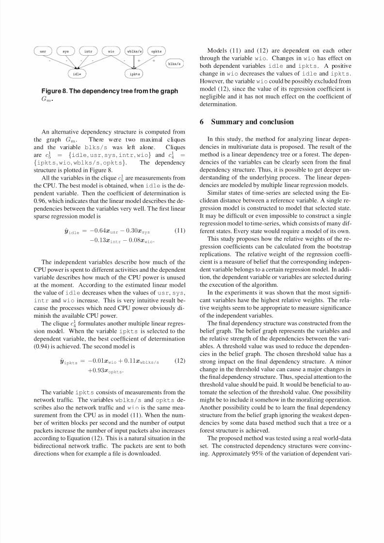
Figure 8. The dependency tree from the graphGm .

An alternative dependency structure is computed fromthe graph Gm . There were two maximal cliquesand the variable blks/s was left alone. Cliquesare c1

5 = {idle , usr , sys , intr , wio } and c14 =

{ipkts , wio , wblks/s , opkts }. The dependencystructure is plotted in Figure 8.

All the variables in the clique c15 are measurements from

the CPU. The best model is obtained, when idle is the de-pendent variable. Then the coefcient of determination is0.96, which indicates that the linear model describes the de-pendencies between the variables very well. The rst linearsparse regression model is

y idle = − 0.64x usr − 0.30x sys (11)

− 0.13x intr − 0.08x wio .

The independent variables describe how much of theCPU power is spent to different activities and the dependentvariable describes how much of the CPU power is unused

at the moment. According to the estimated linear modelthe value of idle decreases when the values of usr , sys ,intr and wio increase. This is very intuitive result be-cause the processes which need CPU power obviously di-minish the available CPU power.

The clique c14 formulates another multiple linear regres-

sion model. When the variable ipkts is selected to thedependent variable, the best coefcient of determination(0.94) is achieved. The second model is

y ipkts = − 0.01x wio + 0 .11x wblks/s (12)

+0 .93x opkts .

The variable ipkts consists of measurements from thenetwork trafc. The variables wblks/s and opkts de-scribes also the network trafc and wio is the same mea-surement from the CPU as in model (11). When the num-ber of written blocks per second and the number of outputpackets increase the number of input packets also increasesaccording to Equation (12). This is a natural situation in thebidirectional network trafc. The packets are sent to bothdirections when for example a le is downloaded.

Models (11) and (12) are dependent on each otherthrough the variable wio . Changes in wio has effect onboth dependent variables idle and ipkts . A positivechange in wio decreases the values of idle and ipkts .However, the variable wio could be possibly excluded frommodel (12), since the value of its regression coefcient isnegligible and it has not much effect on the coefcient of determination.

6 Summary and conclusion

In this study, the method for analyzing linear depen-dencies in multivariate data is proposed. The result of themethod is a linear dependency tree or a forest. The depen-dencies of the variables can be clearly seen from the naldependency structure. Thus, it is possible to get deeper un-derstanding of the underlying process. The linear depen-dencies are modeled by multiple linear regression models.

Similar states of time-series are selected using the Eu-clidean distance between a reference variable. A single re-gression model is constructed to model that selected state.It may be difcult or even impossible to construct a singleregression model to time-series, which consists of many dif-ferent states. Every state would require a model of its own.

This study proposes how the relative weights of the re-gression coefcients can be calculated from the bootstrapreplications. The relative weight of the regression coef-cient is a measure of belief that the corresponding indepen-dent variable belongs to a certain regression model. In addi-tion, the dependent variable or variables are selected during

the execution of the algorithm.In the experiments it was shown that the most signi-

cant variables have the highest relative weights. The rela-tive weights seem to be appropriate to measure signicanceof the independent variables.

The nal dependency structure was constructed from thebelief graph. The belief graph represents the variables andthe relative strength of the dependencies between the vari-ables. A threshold value was used to reduce the dependen-cies in the belief graph. The chosen threshold value has astrong impact on the nal dependency structure. A minorchange in the threshold value can cause a major changes inthe nal dependency structure. Thus, special attention to thethreshold value should be paid. It would be benecial to au-tomate the selection of the threshold value. One possibilitymight be to include it somehow in the moralizing operation.Another possibility could be to learn the nal dependencystructure from the belief graph ignoring the weakest depen-dencies by some data based method such that a tree or aforest structure is achieved.

The proposed method was tested using a real world-dataset. The constructed dependency structures were convinc-ing. Approximately 95% of the variation of dependent vari-



ables was explained by the regression models which wereconstructed from the System data, although no assumptionswere made about the number of linear models. The result-ing dependency structure was almost similar to one shownin Figure 8, when the whole data set was used in the con-struction of the dependency structure. When models (11)and (12) were tested with the excluded data the coefcientsof determination were nearly as good as with the used data.

The nal dependency structure highlights the dependen-cies of the variables in an intelligible way. On the otherhand, it is difcult to measure the level of interpretability.The goodness of the models may be hard to justify if coef-cient of determinations are moderate, but the dependencystructure can still give additional and unexpected informa-tion in co-operation with someone who has specic knowl-edge of the underlying process.

7 Acknowledgements

The authors thank Dr. Esa Alhoniemi for the idea of selecting similar windows from time-series. We also thank for the insightful comments from the reviewers of the paper.

References

[1] L. Breiman. The little bootstrap and other methods fordimensionality selection in regression: X-xed predictionerror. Journal of the American Statistical Association ,87(419):738–754, September 1992.

[2] L. Breiman. Better subset regression using the nonnegative

garrote. Technometrics , 37(4):373–384, November 1995.[3] C. Chow and C. Liu. Approximating discrete probabilitydistributions with dependence trees. IEEE Transactions on Information Theory , 14(3):462–467, May 1968.

[4] J. Copas. Regression, prediction and shrinkage. Journalof the Royal Statistical Society (Series B) , 45(3):311–354,1983.

[5] D. L. Donoho. De-noising by soft-thresholding. IEEE Transactions on Information Theory , 41(3):613–627, May1995.

[6] B. Efron. Bootstrap methods: Another look at the Jackknife.The Annals of Statistics , 7(1):1–26, January 1979.

[7] B. Efron, T. Hastie, I. Johnstone, and R. Tibshirani. Leastangle regression. The Annals of Statistics , 32(2):407–499,

April 2004.[8] B. Efron and R. J. Tibshirani. An Introduction to the Boot-strap . Chapman & Hall, 1993.

[9] M. H. Hansen and B. Yu. Model selection and the principleof minimum description length. Journal of the AmericanStatistical Association , 96(454):746–774, June 2001.

[10] T. Hastie, R. Tibshirani, and J. Friedman. The Elements of Statistical Learning . Springer, 2001.

[11] D. Heckerman, D. M. Chickering, C. Meek, R. Rounthwaite,and C. Kadie. Dependency networks for inference, collab-orative ltering, and data visualization. Journal of Machine Learning Research , 1:49–75, October 2000.

[12] A. E. Hoerl and R. W. Kennard. Ridge regression: Bi-ased estimation for nonorthogonal problems. Technometrics ,12(1):55–67, February 1970.

[13] C. Huang and A. Darwiche. Inference in belief networks:A procedural guide. International Journal of Approximate Reasoning , 15(3):225–263, October 1996.

[14] I. Koch. Enumerating all connected maximal common sub-graphs in two graphs. Theoretical Computer Science , 250(1-2):1–30, January 2001.

[15] F. Kose, W. Weckwerth, T. Linke, and O. Fiehn. Visual-izing plant metabolomic correlation networks using clique-metabolite matrices. Bioinformatics , 17(12):1198–1208,December 2001.

[16] K. Lagus, E. Alhoniemi, and H. Valpola. Independentvariable group analysis. In G. Dorffner, H. Bischof, andK. Hornik, editors, Proceedings of the International Confer-ence on Articial Neural Networks , number 2130 in LectureNotes in Computer Science, pages 203–210. Springer, 2001.

[17] M. Lang, H. Guo, J. E. Odegard, C. S. Burrus, andR. O. Wells. Noise reduction using an undecimated dis-

crete wavelet transform. IEEE Signal Processing Letters ,3(1):10–12, January 1996.

[18] C. L. Mallows. Some comments on C p . Technometrics ,15(4):661–675, November 1973.

[19] C. L. Mallows. More comments on C p . Technometrics ,37(4):362–372, November 1995.

[20] G. M. Maruyama. Basics of Structural Equation Modeling .SAGE Publications, Inc., 1997.

[21] P. Stoica and Y. Selen. Model-order selection. IEEE SignalProcessing Magazine , 21(4):36–47, July 2004.

[22] R. Tibshirani. Regression shrinkage and selection via thelasso. Journal of the Royal Statistical Society. Series B(Methodological) , 58(1):267–288, 1996.

[23] J. Vesanto and J. Hollm´ en. An automated report genera-

tion tool for the data understanding phase. In A. Abraham,L. Jain, and B. J. van der Zwaag, editors, Innovations in In-telligent Systems: Design, Management and Applications ,Studies in Fuzziness and Soft Computing. Springer (Phys-ica) Verlag, 2003.

learning linear dependency trees from multivariate time-series data

Documents