Learning Mean-Field Games

Xin Guo ∗ Anran Hu † Renyuan Xu ‡ Junzi Zhang §

Abstract

This paper presents a general mean-field game (GMFG) framework for simultaneouslearning and decision-making in stochastic games with a large population. It firstestablishes the existence of a unique Nash Equilibrium to this GMFG, and explains thatnaively combining Q-learning with the fixed-point approach in classical MFGs yieldsunstable algorithms. It then proposes a Q-learning algorithm with Boltzmann policy(GMF-Q), with analysis of convergence property and computational complexity. Theexperiments on repeated Ad auction problems demonstrate that this GMF-Q algorithmis efficient and robust in terms of convergence and learning accuracy. Moreover, itsperformance is superior in convergence, stability, and learning ability, when comparedwith existing algorithms for multi-agent reinforcement learning.

1 IntroductionMotivating example. This paper is motivated by the following Ad auction problem foran advertiser. An Ad auction is a stochastic game on an Ad exchange platform amonga large number of players, the advertisers. In between the time a web user requests apage and the time the page is displayed, usually within a millisecond, a Vickrey-type ofsecond-best-price auction is run to incentivize interested advertisers to bid for an Ad slot todisplay advertisement. Each advertiser has limited information before each bid: first, herown valuation for a slot depends on an unknown conversion of clicks for the item; secondly,she, should she win the bid, only knows the reward after the user’s activities on the websiteare finished. In addition, she has a budget constraint in this repeated auction.

The question is, how should she bid in this online sequential repeated game when there isa large population of bidders competing on the Ad platform, with unknown distributions ofthe conversion of clicks and rewards?∗Department of Industrial Engineering & Operations Research, University of California, Berkeley, USA.

Email: xinguo@berkeley.edu†Department of Industrial Engineering & Operations Research, University of California, Berkeley, USA.

Email: anran_hu@berkeley.edu‡Department of Industrial Engineering & Operations Research, University of California, Berkeley, USA.

Email: renyuanxu@berkeley.edu§Institute for Computational & Mathematical Engineering, Stanford University, USA. Email: jun-

ziz@stanford.edu

1

arX

iv:1

901.

0958

5v3

[m

ath.

OC

] 6

Jun

201

9

Besides the Ad auction, there are many real-world problems involving a large number ofplayers and unknown systems. Examples include massive multi-player online role-playinggames [14], high frequency tradings [19], and the sharing economy [9].

Our work. Motivated by these problems, we consider a general framework of simultaneouslearning and decision-making in stochastic games with a large population. We formulatea general mean-field-game (GMFG) with incorporation of action distributions, and withunknown rewards and dynamics. This general framework can also be viewed as a generalizedversion of MFGs of McKean-Vlasov type [1], which is a different paradigm from the classicalMFG. It is also beyond the scope of the existing Q-learning framework for Markov decisionproblem (MDP) with unknown distributions, as MDP is technically equivalent to a singleplayer stochastic game.

On the theory front, this general framework differs from all existing MFGs. We establishunder appropriate technical conditions, the existence and uniqueness of the Nash equilibrium(NE) to this GMFG. On the computational front, we show that naively combining Q-learningwith the three-step fixed-point approach in classical MFGs yields unstable algorithms. We thenpropose a Q-learning algorithm with Boltzmann policy (GMF-Q), establish its convergenceproperty and analyze its computational complexity. Finally, we apply this GMF-Q algorithmto the Ad auction problem, where this GMF-Q algorithm demonstrates its efficiency androbustness in terms of convergence and learning. Moreover, its performance is superior, whencompared with existing algorithms for multi-agent reinforcement learning for convergence,stability, and learning accuracy.

Related works. On learning large population games with mean-field approximations, [30]focuses on inverse reinforcement learning for MFGs without decision making, [31] studies anMARL problem with a first-order mean-field approximation term modeling the interactionbetween one player and all the other finite players, and [17] and [32] consider model-basedadaptive learning for MFGs in specific models (e.g., linear-quadratic and oscillator games).More recently, [25] considers reinforcement learning in the classical MFG setting, and proposesa policy-gradient based algorithm and analyzes the so-called local NE. For learning largepopulation games without mean-field approximation, see [16, 10] and the references therein.

In the specific topic of learning auctions with a large number of advertisers, [4] and [15]explore reinforcement learning techniques to search for social optimal solutions with real-worddata, and [13] uses MFGs to model the auction system with unknown conversion of clickswithin a Bayesian framework.

However, none of these works consider the problem of simultaneous learning and decision-making in a general MFG framework. Neither do they establish the existence and uniquenessof the NE, nor do they present model-free learning algorithms with complexity analysis andconvergence to the NE.

2

2 Framework of General MFG (GMFG)

2.1 Background: classical N-player Markovian game and MFG

Let us first recall the classical N -player game. There are N players in a game. At each stept, the state of player i (= 1, 2, · · · , N) is sit ∈ S ⊆ Rd and she takes an action ait ∈ A ⊆ Rp.Here d, p are positive integers, and S and A are compact (for example, finite) state space andaction space, respectively. Given the current state profile of N -players st = (s1t , . . . , s

Nt ) ∈ SN

and the action ait, player i will receive a reward ri(st, ait) and her state will change to sit+1

according to a transition probability function P i(st, ait).

A Markovian game further restricts the admissible policy/control for player i to be of theform ait = πit(s

t). That is, πit : SN → P(A) maps each state profile s ∈ SN to a randomizedaction, with P(X ) the space of probability measures on space X . The accumulated reward(a.k.a. the value function) for player i, given the initial state profile s and the policy profilesequence πππ := πππt∞t=0 with πππt = (π1

t , . . . , πNt ), is then defined as

V i(s,πππ) := E

[∞∑t=0

γtri(st, ait)∣∣∣s0 = s

], (1)

where γ ∈ (0, 1) is the discount factor, ait ∼ πit(st), and sit+1 ∼ P i(st, a

it). The goal of each

player is to maximize her value function over all admissible policy sequences.In general, this type of stochastic N -player game is notoriously hard to analyze, especially

when N is large. Mean field game (MFG), pioneered by [12] and [18], provides an ingeniousand tractable aggregation approach to approximate the otherwise challenging N -playerstochastic games. The basic idea for an MFG goes as follows. Assume all players areidentical, indistinguishable and interchangeable, when N → ∞, one can view the limitof other players’ states s−it = (s1t , . . . , s

i−1t , si+1

t , . . . , sNt ) as a population state distribution

µt := limN→∞

∑Nj=1,j 6=i 1(s

jt )

N. Due to the homogeneity of the players, one can then focus on a

single (representative) player. That is, in an MFG, one may consider instead the followingoptimization problem,

maximizeπππ V (s,πππ,µµµ) := E[∞∑t=0

γtr(st, at, µt)|s0 = s

]subject to st+1 ∼ P (st, at, µt), at ∼ πt(st, µt),

where πππ := πt∞t=0 denotes the policy sequence and µµµ := µt∞t=0 the distribution flow. Inthis MFG setting, at time t, after the representative player chooses her action at accordingto some policy πt, she will receive reward r(st, at, µt) and her state will evolve under acontrolled stochastic dynamics of a mean-field type P (·|st, at, µt). Here the policy πt dependson both the current state st and the current population state distribution µt such thatπ : S × P(S)→ P(A).

3

2.2 General MFG (GMFG)

In the classical MFG setting, the reward and the dynamic for each player are known. Theydepend only on st the state of the player, at the action of this particular player, and µt thepopulation state distribution. In contrast, in the motivating auction example, the rewardand the dynamic are unknown; they rely on the actions of all players, as well as on st and µt.

We therefore define the following general MFG (GMFG) framework. At time t, after therepresentative player chooses her action at according to some policy π : S × P(S)→ P(A),she will receive a reward r(st, at,Lt) and her state will evolve according to P (·|st, at,Lt),where r and P are possibly unknown. The objective of the player is to solve the followingcontrol problem:

maximizeπππ V (s,πππ,LLL) := E[∞∑t=0

γtr(st, at,Lt)|s0 = s

]subject to st+1 ∼ P (st, at,Lt), at ∼ πt(st,Lt).

(GMFG)

Here, LLL := Lt∞t=0, with Lt = Pst,at ∈ P(S × A) the joint distribution of the state andthe action (i.e., the population state-action pair). Lt has marginal distributions αt for thepopulation action and µt for the population state.

In this framework, we adopt the well-known Nash Equilibrium (NE) for analyzing stochasticgames.

Definition 2.1 (NE for GMFGs). In (GMFG), a player-population profile (πππ?,LLL?) :=(π?t ∞t=0, L?t∞t=0) is called an NE if

1. (Single player side) Fix LLL?, for any policy sequence πππ := πt∞t=0 and any initial states ∈ S,

V (s,πππ?,LLL?) ≥ V (s,πππ,LLL?) . (2)

2. (Population side) Pst,at = L?t for all t ≥ 0, where st, at∞t=0 is the dynamics under thepolicy sequence πππ? starting from s0 ∼ µ?0, with at ∼ π?t (st, µ

?t ), st+1 ∼ P (·|st, at,L?t ),

and µ?t being the population state marginal of L?t .

The single player side condition captures the optimality of πππ?, when the population side isfixed. The population side condition ensures the “consistency” of the solution: it guaranteesthat the state and action distribution flow of the single player does match the populationstate and action sequence LLL?.

2.3 Example: GMFG for the repeated auction

Now, consider the repeated Vickrey auction with a budget constraint in Section 1. Takea representative advertiser in the auction. Denote st ∈ 0, 1, 2, · · · , smax as the budget ofthis player at time t, where smax ∈ N+ is the maximum budget allowed on the Ad exchangewith a unit bidding price. Denote at as the bid price submitted by this player and αt as the

4

bidding/(action) distribution of the population. The reward for this advertiser with bid atand budget st is

rt = IwMt =1

[(vt − aMt )− (1 + ρ)Ist<aMt (aMt − st)

]. (3)

Here wMt takes values 1 and 0, with wMt = 1 meaning this player winning the bid and 0otherwise. The probability of winning the bid would depend on M , the index for the gameintensity, and αt. (See discussion on M in Appendix H.1.) The conversion of clicks at time tis vt and follows an unknown distribution. aMt is the value of the second largest bid at time t,taking values from 0 to smax, and depends on both M and Lt. Should the player win the bid,the reward rt consists of two parts, corresponding to the two terms in (3). The first term isthe profit of wining the auction, as the winner only needs to pay for the second best bid aMin a Vickrey auction. The second term is the penalty of overshooting if the payment exceedsher budget, with a penalty rate ρ. At each time t, the budget dynamics st follows,

st+1 =

st, wMt 6= 1,st − aMt , wMt = 1 and aMt ≤ st,0, wMt = 1 and aMt > st.

That is, if this player does not win the bid, the budget will remain the same. If she winsand has enough money to pay, her budget will decrease from st to st − aMt . However, if shewins but does not have enough money, her budget will be 0 after the payment and there willbe a penalty in the reward function. Note that in this game, both the rewards rt and thedynamics st are unknown a priori.

In practice, one often modifies the dynamics of st+1 with a non-negative random budgetfulfillment ∆(st+1) after the auction clearing [8], such that

st+1 = st+1 + ∆(st+1). (4)

One may see some particular choices of ∆(st+1) in the experiment section (Section 5).

3 Solution for GMFGsWe now establish the existence and uniqueness of the NE to (GMFG), by generalizing theclassical fixed-point approach for MFGs to this GMFG setting. (See [12] and [18] for theclassical case). It consists of three steps.

Step A. Fix LLL := Lt∞t=0, (GMFG) becomes the classical optimization problem. Indeed,with LLL fixed, the population state distribution sequence µµµ := µt∞t=0 is also fixed, hence thespace of admissible policies is reduced to the single-player case. Solving (GMFG) is nowreduced to finding a policy sequence π?t,LLL ∈ Π := π |π : S → P(A) over all admissibleπππ = πt∞t=0, to maximize

V (s,πππ,LLL) := E[∞∑t=0

γtr(st, at,Lt)|s0 = s

],

subject to st+1 ∼ P (st, at,Lt), at ∼ πt(st,Lt).

5

Moreover, given this fixed LLL sequence and the solution πππ?LLL := π?t,LLL∞t=0, one can define amapping from the fixed population distribution sequence LLL to an arbitrarily chosen optimalrandomized policy sequence. That is,

Γ1 : P(S ×A)∞t=0 → Π∞t=0,

such that πππ?LLL = Γ1(LLL). Note that this πππ?LLL sequence satisfies the single player side conditionin Definition 2.1 for the population state-action pair sequence LLL. That is, V (s,πππ?LLL,LLL) ≥V (s,πππ,LLL) , for any policy sequence πππ = πt∞t=0 and any initial state s ∈ S.

As in the classical MFG literature [12], a feedback regularity (FR) condition is needed forthe analysis of Step A.

Assumption 1. There exists a constant d1 ≥ 0, such that for any LLL,LLL′ ∈ P(S ×A)∞t=0,

D(Γ1(LLL),Γ1(LLL′)) ≤ d1W1(LLL,LLL′), (5)

where

D(πππ,πππ′) := sups∈SW1(πππ(s),πππ′(s)) = sup

s∈Ssupt∈N

W1(πt(s), π′t(s)),

W1(LLL,LLL′) := supt∈N

W1(Lt,L′t),(6)

and W1 is the `1-Wasserstein distance between probability measures [7, 28, 23].

Step B. Based on the analysis in Step A and πππ?LLL = π?t,LLL∞t=0, update the initial sequenceLLL to LLL′ following the controlled dynamics P (·|st, at,Lt).

Accordingly, for any admissible policy sequence πππ ∈ Π∞t=0 and a joint population state-action pair sequence LLL ∈ P(S ×A)∞t=0, define a mapping Γ2 : Π∞t=0 × P(S ×A)∞t=0 →P(S ×A)∞t=0 as follows:

Γ2(πππ,LLL) := LLL = Pst,at∞t=0, (7)

where st+1 ∼ µtP (·|·, at,Lt), at ∼ πt(st), s0 ∼ µ0, and µt is the population state marginal ofLt.

One needs a standard assumption in this step.

Assumption 2. There exist constants d2, d3 ≥ 0, such that for any admissible policysequences πππ,πππ1,πππ2 and joint distribution sequences LLL,LLL1,LLL2,

W1(Γ2(πππ1,LLL),Γ2(πππ

2,LLL)) ≤ d2D(πππ1,πππ2), (8)

W1(Γ2(πππ,LLL1),Γ2(πππ,LLL2)) ≤ d3W1(LLL1,LLL2). (9)

Assumption 2 can be reduced to Lipschitz continuity and boundedness of the transitiondynamics P . (See the Appendix for more details.)

6

Step C. Repeat Step A and Step B until LLL′ matches LLL.This step is to take care of the population side condition. To ensure the convergence

of the combined step A and step B, it suffices if Γ : P(S × A)∞t=0 → P(S × A)∞t=0 is acontractive mapping under the W1 distance, with Γ(LLL) := Γ2(Γ1(LLL),LLL). Then by the Banachfixed point theorem and the completeness of the related metric spaces, there exists a uniqueNE to the GMFG.

In summary, we have

Theorem 1 (Existence and Uniqueness of GMFG solution). Given Assumptions 1 and 2,and assume d1d2 + d3 < 1. Then there exists a unique NE to (GMFG).

4 RL Algorithms for GMFGsIn this section, we design the computational algorithm for the GMFG. Since the rewardand transition distributions are unknown, this is simultaneously learning the system andfinding the NE of the game. We will focus on the case with finite state and action spaces,i.e., |S|, |A| < ∞. We will look for stationary (time independent) NEs. Accordingly, weabbreviate πππ := π∞t=0 and LLL : L∞t=0 as π and L, respectively. This stationarity propertyenables developing appropriate time-independent Q-learning algorithm, suitable for an infinitetime horizon game. Modification from the GMFG framework to this special stationary settingis straightforward, and is left in the Appendix.

The algorithm consists of two steps, parallel to Step A and Step B in Section 3.

Step 1: Q-learning with stability for fixed L. With L fixed, it becomes a standardlearning problem for an infinite horizon MDP. We will focus on the Q-learning algorithm[26, 24].

The Q-learning algorithm approximates the value iteration by stochastic approximation.At each step with the state s and an action a, the system reaches state s′ according to thecontrolled dynamics and the Q-function is updated according to

QL(s, a)← (1− βt(s, a))QL(s, a) + βt(s, a) [r(s, a,L) + γmaxaQL(s′, a)] , (10)

where the step size βt(s, a) can be chosen as ([5])

βt(s, a) =

|#(s, a, t) + 1|−h, (s, a) = (st, at),

0, otherwise.

with h ∈ (1/2, 1). Here #(s, a, t) is the number of times up to time t that one visits thepair (s, a). The algorithm then proceeds to choose action a′ based on QL with appropriateexploration strategies, including the ε-greedy strategy.

After obtaining the approximate Q?L, in order to retrieve an approximately optimal policy,

it would be natural to define an argmax-e operator so that actions with equal maximumQ-values would have equal probabilities to be selected. Unfortunately, the discontinuity

7

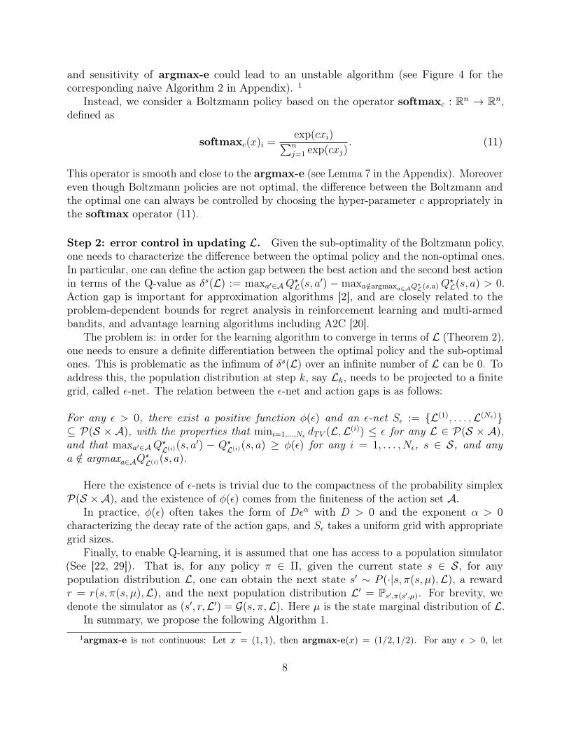
and sensitivity of argmax-e could lead to an unstable algorithm (see Figure 4 for thecorresponding naive Algorithm 2 in Appendix). 1

Instead, we consider a Boltzmann policy based on the operator softmaxc : Rn → Rn,defined as

softmaxc(x)i =exp(cxi)∑nj=1 exp(cxj)

. (11)

This operator is smooth and close to the argmax-e (see Lemma 7 in the Appendix). Moreovereven though Boltzmann policies are not optimal, the difference between the Boltzmann andthe optimal one can always be controlled by choosing the hyper-parameter c appropriately inthe softmax operator (11).

Step 2: error control in updating L. Given the sub-optimality of the Boltzmann policy,one needs to characterize the difference between the optimal policy and the non-optimal ones.In particular, one can define the action gap between the best action and the second best actionin terms of the Q-value as δs(L) := maxa′∈AQ

?L(s, a′) − maxa/∈argmaxa∈AQ?L(s,a)Q

?L(s, a) > 0.

Action gap is important for approximation algorithms [2], and are closely related to theproblem-dependent bounds for regret analysis in reinforcement learning and multi-armedbandits, and advantage learning algorithms including A2C [20].

The problem is: in order for the learning algorithm to converge in terms of L (Theorem 2),one needs to ensure a definite differentiation between the optimal policy and the sub-optimalones. This is problematic as the infimum of δs(L) over an infinite number of L can be 0. Toaddress this, the population distribution at step k, say Lk, needs to be projected to a finitegrid, called ε-net. The relation between the ε-net and action gaps is as follows:

For any ε > 0, there exist a positive function φ(ε) and an ε-net Sε := L(1), . . . ,L(Nε)⊆ P(S × A), with the properties that mini=1,...,Nε dTV (L,L(i)) ≤ ε for any L ∈ P(S × A),and that maxa′∈AQ

?L(i)(s, a

′) − Q?L(i)(s, a) ≥ φ(ε) for any i = 1, . . . , Nε, s ∈ S, and any

a /∈ argmaxa∈AQ?L(i)(s, a).

Here the existence of ε-nets is trivial due to the compactness of the probability simplexP(S ×A), and the existence of φ(ε) comes from the finiteness of the action set A.

In practice, φ(ε) often takes the form of Dεα with D > 0 and the exponent α > 0characterizing the decay rate of the action gaps, and Sε takes a uniform grid with appropriategrid sizes.

Finally, to enable Q-learning, it is assumed that one has access to a population simulator(See [22, 29]). That is, for any policy π ∈ Π, given the current state s ∈ S, for anypopulation distribution L, one can obtain the next state s′ ∼ P (·|s, π(s, µ),L), a rewardr = r(s, π(s, µ),L), and the next population distribution L′ = Ps′,π(s′,µ). For brevity, wedenote the simulator as (s′, r,L′) = G(s, π,L). Here µ is the state marginal distribution of L.

In summary, we propose the following Algorithm 1.1argmax-e is not continuous: Let x = (1, 1), then argmax-e(x) = (1/2, 1/2). For any ε > 0, let

8

Algorithm 1 Q-learning for GMFGs (GMF-Q)1: Input: Initial L0, tolerance ε > 0.2: for k = 0, 1, · · · do3: Perform Q-learning for Tk iterations to find the approximate Q-function Q?

k(s, a) =Q?Lk(s, a) of an MDP with dynamics PLk(s′|s, a) and rewards rLk(s, a).

4: Compute πk ∈ Π with πk(s) = softmaxc(Q?k(s, ·)).

5: Sample s ∼ µk, where µk is the population state marginal of Lk, and obtain Lk+1 fromG(s, πk,Lk).

6: Find Lk+1 = ProjSε(Lk+1)7: end for

Here ProjSε(L) = argminL(1),...,L(Nε)dTV (L(i),L). See Lemma 8 and Theorem 2 for detailsabout the choices of hyper-parameters c and Tk.

In the special case when the rewards rL and transition dynamics P (·|s, a,L) are known,one can replace the Q-learning step in the above Algorithm 1 by a value iteration, resultingin the GMF-V Algorithm 3 in the Appendix.

We next show the convergence of this GMF-Q algorithm (Algorithm 1) to an ε-Nash of(GMFG), with complexity analysis.

Theorem 2 (Convergence and complexity of GMF-Q). Assume the same conditions inTheorem 1 and Lemma 8 in the Appendix. For any tolerances ε, δ > 0, set δk = δ/Kε,η,εk = (k + 1)−(1+η) for some η ∈ (0, 1] (k = 0, . . . , Kε,η − 1), Tk = TMLk (δk, εk) (definedin Lemma 8 in the Appendix) and c = log(1/ε)

φ(ε). Then with probability at least 1 − 2δ,

W1(LKε,η ,L?) ≤ Cε.Moreover, the total number of iterations T =

∑Kε,η−1k=0 TMLk (δk, εk) is bounded by

T = O(K

1+ 4h

ε,η (log(Kε,η/δ))2

1−h+2h+3). (12)

Here Kε,η :=⌈2 max

(ηε)−1/η, logd(ε/maxdiam(S)diam(A), 1) + 1)

⌉is the number of

outer iterations, h is the step-size exponent in Q-learning (defined in Lemma 8 in theAppendix), and the constant C is independent of δ, ε and η.

The proof of Theorem 2 in the Appendix depends on the Lipschitz continuity of thesoftmax operator [6], the closeness between softmax and the argmax-e (Lemma 7 in theAppendix), and the complexity of Q-learning for the MDP (Lemma 8 in the Appendix).Lemma 8 also provides guidance on how to choose the number of inner iterations Tk inAlgorithm 1.

y = (1, 1− ε), then argmax-e(y) = (1, 0).

9

5 Experiment: repeated auction gameIn this section, we report the performance of the proposed GMF-Q Algorithm. The objectivesof the experiments include 1) testing the convergence, stability, and learning ability of GMF-Qin the GMFG setting, and 2) comparing GMF-Q with existing multi-agent reinforcementlearning algorithms, including IL algorithm and MF-Q algorithm.

We take the GMFG framework for the repeated auction game from Section 2.3. Hereeach advertiser learns to bid in the auction with a budget constraint.

Parameters. The model parameters are set as: |S| = |A| = 10, the overbidding penaltyρ = 0.2, the distributions of the conversion rate v ∼ uniform[4], and the competition intensityindex M = 5. The random fulfillment is chosen as: if s < smax, ∆(s) = 1 with probability 1

2

and ∆(s) = 0 with probability 12; if s = smax, ∆(s) = 0.

The algorithm parameters are (unless otherwise specified): the temperature parameterc = 4.0, the discount factor γ = 0.8, the parameter h from Lemma 8 in the Appendix beingh = 0.87, and the baseline inner iteration being 2000. Recall that for GMF-Q, both v andthe dynamics of P for s are unknown a priori. The 90%-confidence intervals are calculatedwith 20 sample paths.

Performance evaluation in the GMFG setting. Our experiment shows that the GMF-Q Algorithm is efficient and robust, and learns well.

Convergence and stability of GMF-Q. GMF-Q is efficient and robust. First, GMF-Qconverges after about 10 outer iterations; secondly, as the number of inner iterations increases,the error decreases (Figure 2); and finally, the convergence is robust with respect to both thechange of number of states and the initial population distribution (Figure 3).

In contrast, the Naive algorithm does not converge even with 10000 inner iterations, andthe joint distribution Lt keeps fluctuating (Figure 4).

Learning accuracy of GMF-Q. GMF-Q learns well. Its learning accuracy is tested againstits special form GMF-V (Appendix G), with the latter assuming a known distribution ofconversation rate v and the dynamics P for the budget s. The relative L2 distance betweenthe Q-tables of these two algorithms is ∆Q :=

‖QGMF-V−QGMF-Q‖2‖QGMF-V‖2 = 0.098879. This implies

that GMF-Q learns the true GMFG solution with 90-percent accuracy with 10000 inneriterations.

The heatmap in Figure 1(a) is the Q-table for GMF-Q Algorithm after 20 outer iterations.Within each outer iteration, there are TGMF-Q

k = 10000 inner iterations. The heatmap inFigure 1(b) is the Q-table for GMF-Q Algorithm after 20 outer iterations. Within each outeriteration, there are TGMF-V

k = 5000 inner iterations.

Comparison with existing algorithms for N-player games. To test the effectivenessof GMF-Q for approximating N -player games, we next compare GMF-Q with IL algorithm

10

Table 1: Q-table with TGMF-Vk = 5000.

TGMF-Qk 1000 3000 5000 10000∆Q 0.21263 0.1294 0.10258 0.0989

(a) GMF-Q. (b) GMF-V.

Figure 1: Q-tables: GMF-Q vs. GMF-V.

0 2 4 6 8 10 12 14 16 18outer iteration

0.00

0.01

0.02

0.03

0.04

0.05

0.06

|t+

1t| 1

50020005000

Figure 2: Convergence with differentnumber of inner iterations.

0 2 4 6 8 10 12 14 16 18outer iteration

0.0

0.2

0.4

0.6

0.8

1.0

1.2

|t

t+1| 1

1030100

Figure 3: Convergence with differentnumber of states.

11

0 20 40 60 80 100outer iteration

0.0

0.2

0.4

0.6

0.8

1.0

|t

t+1|

(a) fluctuation in l∞.

0 20 40 60 80 100outer iteration

1.3

1.4

1.5

1.6

1.7

1.8

1.9

2.0

|t

t+1| 1

(b) fluctuation in l1.

Figure 4: Fluctuations of Naive Algorithm (30 sample paths).

0 10000 20000 30000 40000 50000 60000 70000 80000

0.0

0.1

0.2

0.3

0.4

0.5

0.6

0.7

c()

MF-QILGMF-Q

(a) |S| = |A| = 10, N = 20.

0 10000 20000 30000 40000 50000 60000 70000 80000

0.0

0.1

0.2

0.3

0.4

0.5

0.6

0.7

0.8

c()

MF-QILGMF-Q

(b) |S| = |A| = 20, N = 20.

0 10000 20000 30000 40000 50000 60000 70000 80000

0.0

0.1

0.2

0.3

0.4

0.5

0.6

0.7

c()

MF-QILGMF-Q

(c) |S| = |A| = 10, N = 40.

Figure 5: Learning accuracy based on C(πππ).

12

and MF-Q algorithm. IL algorithm [27] considers N independent players and each playersolves a decentralized reinforcement learning problem ignoring other players in the system.The MF-Q algorithm [31] extends the NASH-Q Learning algorithm for the N -player gameintroduced in [11], adds the aggregate actions (aaa−i =

∑j 6=i aj

N−1 ) from the opponents, and worksfor the class of games where the interactions are only through the average actions of Nplayers.

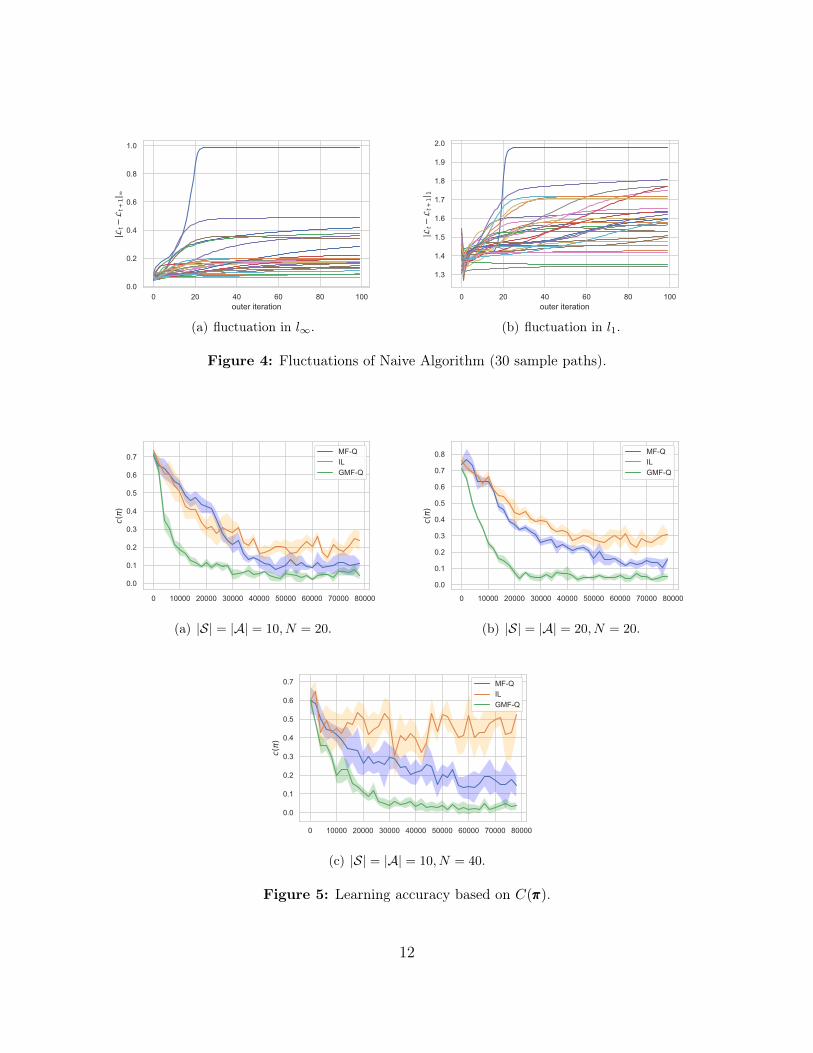
Performance metric. We adopt the following metric to measure the difference between agiven policy π and an NE (here ε0 > 0 is a safeguard, and is taken as 0.1 in the experiments):

C(πππ) =1

N |S|N∑N

i=1

∑sss∈SN

maxπi Vi(sss, (πππ−i, πi))− Vi(sss,πππ)

|maxπi Vi(sss, (πππ−i, πi))|+ ε0.

Clearly C(πππ) ≥ 0, and C(πππ∗) = 0 if and only if πππ∗ is an NE. Policy arg maxπi Vi(sss, (πππ−i, πi))

is called the best response to πππ−i. A similar metric without normalization has been adoptedin [21].

Our experiment (Figure 5) shows that GMF-Q is superior in terms of convergence rate,accuracy, and stability for approximating an N -player game: GMF-Q converges faster thanIL and MF-Q, with the smallest error, and with the lowest variance, as ε-net improves thestability.

For instance, when N = 20, IL Algorithm converges with the largest error 0.220. Theerror from MF-Q is 0.101, smaller than IL but still bigger than the error from GMF-Q. TheGMF-Q converges with the lowest error 0.065. Moreover, as N increases, the error of GMF-Qdeceases while the errors of both MF-Q and IL increase significantly. As |S| and |A| increase,GMF-Q is robust with respect to this increase of dimensionality, while both MF-Q and ILclearly suffer from the increase of the dimensionality with decreased convergence rate andaccuracy. Therefore, GMF-Q is more scalable than IL and MF-Q, when the system is complexand the number of players N is large.

6 ConclusionThis paper builds a GMFG framework for simultaneous learning and decision-making, es-tablishes the existence and uniqueness of NE, and proposes a Q-learning algorithm GMF-Qwith convergence and complexity analysis. Experiments demonstrate superior performance ofGMF-Q.

References[1] B. Acciaio, J. Backhoff, and R. Carmona. Extended mean field control problems:

stochastic maximum principle and transport perspective. Arxiv Preprint:1802.05754,2018.

13

[2] M. G. Bellemare, G. Ostrovski, A. Guez, P. S. Thomas, and R. Munos. Increasing theaction gap: new operators for reinforcement learning. In AAAI Conference on ArtificialIntelligence, pages 1476–1483, 2016.

[3] F. Bolley. Separability and completeness for the Wasserstein distance. Séminaire deProbabilités XLI, pages 371–377, 2008.

[4] H. Cai, K. Ren, W. Zhang, K. Malialis, J. Wang, Y. Yu, and D. Guo. Real-time biddingby reinforcement learning in display advertising. In Proceedings of the Tenth ACMInternational Conference on Web Search and Data Mining, pages 661–670. ACM, 2017.

[5] E. Even-Dar and Y. Mansour. Learning rates for Q-learning. Journal of MachineLearning Research, 5(Dec):1–25, 2003.

[6] B. Gao and L. Pavel. On the properties of the softmax function with application ingame theory and reinforcement learning. Arxiv Preprint:1704.00805, 2017.

[7] A. L. Gibbs and F. E. Su. On choosing and bounding probability metrics. InternationalStatistical Review, 70(3):419–435, 2002.

[8] R. Gummadi, P. Key, and A. Proutiere. Repeated auctions under budget constraints:Optimal bidding strategies and equilibria. In the Eighth Ad Auction Workshop, 2012.

[9] J. Hamari, M. Sjöklint, and A. Ukkonen. The sharing economy: Why people participatein collaborative consumption. Journal of the Association for Information Science andTechnology, 67(9):2047–2059, 2016.

[10] P. Hernandez-Leal, B. Kartal, and M. E. Taylor. Is multiagent deep reinforcementlearning the answer or the question? A brief survey. Arxiv Preprint:1810.05587, 2018.

[11] J. Hu and M. P. Wellman. Nash Q-learning for general-sum stochastic games. Journalof Machine Learning Research, 4(Nov):1039–1069, 2003.

[12] M. Huang, R. P. Malhamé, and P. E. Caines. Large population stochastic dynamicgames: closed-loop McKean-Vlasov systems and the Nash certainty equivalence principle.Communications in Information & Systems, 6(3):221–252, 2006.

[13] K. Iyer, R. Johari, and M. Sundararajan. Mean field equilibria of dynamic auctions withlearning. ACM SIGecom Exchanges, 10(3):10–14, 2011.

[14] S. H. Jeong, A. R. Kang, and H. K. Kim. Analysis of game bot’s behavioral characteristicsin social interaction networks of MMORPG. ACM SIGCOMM Computer CommunicationReview, 45(4):99–100, 2015.

[15] J. Jin, C. Song, H. Li, K. Gai, J. Wang, and W. Zhang. Real-time bidding withmulti-agent reinforcement learning in display advertising. Arxiv Preprint:1802.09756,2018.

14

[16] S. Kapoor. Multi-agent reinforcement learning: A report on challenges and approaches.Arxiv Preprint:1807.09427, 2018.

[17] A. C Kizilkale and P. E Caines. Mean field stochastic adaptive control. IEEE Transactionson Automatic Control, 58(4):905–920, 2013.

[18] J-M. Lasry and P-L. Lions. Mean field games. Japanese Journal of Mathematics,2(1):229–260, 2007.

[19] C-A. Lehalle and C. Mouzouni. A mean field game of portfolio trading and its conse-quences on perceived correlations. ArXiv Preprint:1902.09606, 2019.

[20] V. M. Minh, A. P. Badia, M. Mirza, A. Graves, T. P. Lillicrap, T. Harley, D. Silver, andK. Kavukcuoglu. Asynchronous methods for deep reinforcement learning. In InternationalConference on Machine Learning, 2016.

[21] J. Pérolat, B. Piot, and O. Pietquin. Actor-critic fictitious play in simultaneous movemultistage games. In International Conference on Artificial Intelligence and Statistics,2018.

[22] J. Pérolat, F. Strub, B. Piot, and O. Pietquin. Learning Nash equilibrium for general-sumMarkov games from batch data. Arxiv Preprint:1606.08718, 2016.

[23] G. Peyré and M. Cuturi. Computational optimal transport. Foundations and Trends inMachine Learning, 11(5-6):355–607, 2019.

[24] B. Recht. A tour of reinforcement learning: The view from continuous control. AnnualReview of Control, Robotics, and Autonomous Systems, 2018.

[25] J. Subramanian and A. Mahajan. Reinforcement learning in stationary mean-field games.International Conference on Autonomous Agents and Multiagent Systems, 2019.

[26] R. S. Sutton and A. G. Barto. Reinforcement learning: An introduction. MIT press,2018.

[27] M. Tan. Multi-agent reinforcement learning: independent vs. cooperative agents. InInternational Conference on Machine Learning, pages 330–337, 1993.

[28] C. Villani. Optimal transport: old and new, volume 338. Springer Science & BusinessMedia, 2008.

[29] H. T. Wai, Z. Yang, Z. Wang, and M. Hong. Multi-agent reinforcement learning viadouble averaging primal-dual optimization. In Advances in Neural Information ProcessingSystems, pages 9672–9683, 2018.

[30] J. Yang, X. Ye, R. Trivedi, H. Xu, and H. Zha. Deep mean field games for learningoptimal behavior policy of large populations. Arxiv Preprint:1711.03156, 2017.

15

[31] Y. Yang, R. Luo, M. Li, M. Zhou, W. Zhang, and J. Wang. Mean field multi-agentreinforcement learning. Arxiv Preprint:1802.05438, 2018.

[32] H. Yin, P. G. Mehta, S. P. Meyn, and U. V. Shanbhag. Learning in mean-field games.IEEE Transactions on Automatic Control, 59(3):629–644, 2014.

16

A Distance metrics and completenessThis section reviews some basic properties of the Wasserstein distance. It then proves thatthe metrics defined in the main text are indeed distance functions and define complete metricspaces.

`1-Wasserstein distance and dual representation. The `1 Wasserstein distance overP(X ) for X ⊆ Rk is defined as

W1(ν, ν′) := inf

M∈M(ν,ν′)

∫X×X‖x− y‖2dM(x, y). (13)

whereM(ν, ν ′) is the set of all measures (couplings) on X × X , with marginals ν and ν ′ onthe two components, respectively.

The Kantorovich duality theorem enables the following equivalent dual representation ofW1:

W1(ν, ν′) = sup

‖f‖L≤1

∣∣∣∣∫Xfdν −

∫Xfdν ′

∣∣∣∣ , (14)

where the supremum is taken over all 1-Lipschitz functions f , i.e., f satisfying |f(x)−f(y)| ≤‖x− y‖2 for all x, y ∈ X .

The Wasserstein distance W1 can also be related to the total variation distance via thefollowing inequalities [7]:

dmin(X )dTV (ν, ν ′) ≤ W1(ν, ν′) ≤ diam(X )dTV (ν, ν ′), (15)

where dmin(X ) = minx 6=y∈X ‖x− y‖2, which is guaranteed to be positive when X is finite.When S and A are compact, for any compact subset X ⊆ Rk, and for any ν, ν ′ ∈ P(X ),

W1(ν, ν′) ≤ diam(X )dTV (ν, ν ′) ≤ diam(X ) < ∞, where diam(X ) = supx,y∈X ‖x − y‖2 and

dTV is the total variation distance. Moreover, one can verify

Lemma 3. Both D and W1 are distance functions, and they are finite for any input distri-bution pairs. In addition, both (Π∞t=0, D) and (P(S × A)∞t=0,W1) are complete metricspaces.

These facts enable the usage of Banach fixed-point mapping theorem for the proof ofexistence and uniqueness (Theorems 1 and 4).

Proof of Lemma 3. It is known that for any compact set X ⊆ Rk, (P(X ),W1) definesa complete metric space [3]. Since W1(ν, ν

′) ≤ diam(X ) is uniformly bounded for anyν, ν ′ ∈ P(X ), we know that W1(LLL,LLL′) ≤ diam(X ) and D(πππ,π′π′π′) ≤ diam(X ) as well, so theyare both finite for any input distribution pairs. It is clear that they are distance functionsbased on the fact that W1 is a distance function.

Finally, we show the completeness of the two metric spaces (Π∞t=0, D) and (P(S ×A)∞t=0,W1). Take (Π∞t=0, D) for example. Suppose that πππk is a Cauchy sequence in

17

(Π∞t=0, D). Then for any ε > 0, there exists a positive integer N , such that for anym, n ≥ N ,

D(πππn,πππm) ≤ ε =⇒ W1(πnt (s), πmt (s)) ≤ ε for any s ∈ S, t ∈ N, (16)

which implies that πkt (s) forms a Cauchy sequence in (P(A),W1), and hence by the complete-ness of (P(A),W1), πkt (s) converges to some πt(s) ∈ P(A). As a result, πππn → πππ ∈ Π∞t=0

under metric D, which shows that (Π∞t=0, D) is complete.The completeness of (P(S ×A)∞t=0,W1) can be proved similarly.

The same argument for Lemma 3 shows that both D and W1 are distance functionsand are finite for any input distribution pairs, with both (Π, D) and (P(S ×A),W1) againcomplete metric spaces.

B Existence and uniqueness for stationary NE of GMFGsDefinition B.1 (Stationary NE for GMFGs). In (GMFG), a player-population profile (π?,L?) is called a stationary NE if

1. (Single player side) For any policy π and any initial state s ∈ S,

V (s, π?,L?) ≥ V (s, π,L?) . (17)

2. (Population side) Pst,at = L? for all t ≥ 0, where st, at∞t=0 is the dynamics underthe policy π? starting from s0 ∼ µ?, with at ∼ π?(st, µ

?), st+1 ∼ P (·|st, at,L?), and µ?being the population state marginal of L?.

The existence and uniqueness of the NE to (GMFG) in the stationary setting can beestablished by modifying appropriately the same fixed-point approach for the GMFG in themain text.

Step 1. Fix L, the GMFG becomes the classical optimization problem. That is, solving(GMFG) is now reduced to finding a policy π?L ∈ Π := π |π : S → P(A) to maximize

V (s, π,L) := E[∞∑t=0

γtr(st, at,L)|s0 = s

],

subject to st+1 ∼ P (st, at,L), at ∼ πt(st,L).

Now given this fixed L and the solution π?L to the above optimization problem, one can againdefine

Γ1 : P(S ×A)→ Π,

such that π?L = Γ1(L). Note that this π?L satisfies the single player side condition for thepopulation state-action pair L,

V (s, π?L,L) ≥ V (s, π,L) , (18)

for any policy π and any initial state s ∈ S.Accordingly, a similar feedback regularity (FR) condition is needed in this step.

18

Assumption 3. There exists a constant d1 ≥ 0, such that for any L,L′ ∈ P(S ×A),

D(Γ1(L),Γ1(L′)) ≤ d1W1(L,L′), (19)

where

D(π, π′) := sups∈S

W1(π(s), π′(s)), (20)

and W1 is the `1-Wasserstein distance (a.k.a. earth mover distance) between probabilitymeasures.

Step 2. Based on the analysis of Step 1 and π?L, update the initial L to L′ following thecontrolled dynamics P (·|st, at,L).

Accordingly, define a mapping Γ2 : Π× P(S ×A)→ P(S ×A) as follows:

Γ2(π,L) := L = Ps1,a1 , (21)

where a1 ∼ π(s1), s1 ∼ µP (·|·, a0,L), a0 ∼ π(s0), s0 ∼ µ, and µ is the population statemarginal of L.

One also needs a similar assumption in this step.

Assumption 4. There exist constants d2, d3 ≥ 0, such that for any admissible policiesπ, π1, π2 and joint distributions L,L1,L2,

W1(Γ2(π1,L),Γ2(π2,L)) ≤ d2D(π1, π2), (22)

W1(Γ2(π,L1),Γ2(π,L2)) ≤ d3W1(L1,L2). (23)

Step 3. Repeat until L′ matches L.This step is to ensure the population side condition. To ensure the convergence of the

combined step one and step two, it suffices if Γ : P(S × A) → P(S × A) with Γ(L) :=Γ2(Γ1(L),L) is a contractive mapping (under the W1 distance).

Similar to the proof of Theorem 1, again by the Banach fixed point theorem and thecompleteness of the related metric spaces, there exists a unique stationary NE of the GMFG.That is,

Theorem 4 (Existence and Uniqueness of stationary MFG solution). Given Assumptions 3and 4, and assume d1d2 + d3 < 1. Then there exists a unique stationary NE to (GMFG).

19

C Additional comments on assumptionsAs mentioned in the main text, the single player side Assumption 1 and its counterpartAssumption 3 for the stationary version correspond to the feedback regularity (FR) conditionin the classical MFG literature. Here we add some comments on the population sideAssumption 2 and its stationary version Assumption 4. For simplicity and clarity, let usconsider the stationary case with finite state and action spaces. Then we have the followingresult.

Lemma 5. Suppose that maxs,a,L,s′ P (s′|s, a,L) ≤ c1, and that P (s′|s, a, ·) is c2-Lipschitz inW1, i.e.,

|P (s′|s, a,L1)− P (s′|s, a,L2)| ≤ c2W1(L1,L2). (24)

Then in Assumption 4, d2 and d3 can be chosen as

d2 =2diam(S)diam(A)|S|c1

dmin(A)(25)

and d3 = diam(S)diam(A)c22

, respectively.

Lemma 5 provides an explicit characterization of the population side assumptions basedonly on the boundedness and Lipschitz properties of the transition dynamics P . In particular,c1 becomes smaller when the transition dynamics becomes more diverse and the state spacebecomes larger.

Proof. (Lemma 5) We begin by noticing that L′ = Γ2(π,L) can be expanded and computedas follows:

µ′(s′) =∑

s∈S,a∈Aµ(s)P (s′|s, a,L)π(s, a), L′(s′, a′) = µ′(s′)π(s′, a′), (26)

where µ is the state marginal distribution of L.Now by the inequalities (15), we have

W1(Γ2(π1,L),Γ2(π2,L)) ≤ diam(S ×A)dTV (Γ2(π1,L),Γ2(π2,L))

=diam(S ×A)

2

∑s′∈S,a′∈A

∣∣∣∣∣ ∑s∈S,a∈A

µ(s)P (s′|s, a,L) (π1(s, a)π1(s′, a′)− π2(s, a)π2(s

′, a′))

∣∣∣∣∣≤diam(S ×A)

2maxs,a,L,s′

P (s′|s, a,L)∑

s,a,s′,a′

µ(s)(π1(s, a) + π2(s, a))|π1(s′, a′)− π2(s′, a′)|

≤diam(S ×A)

2maxs,a,L,s′

P (s′|s, a,L)∑s′,a′

|π1(s′, a′)− π2(s′, a′)| · (1 + 1)

=2diam(S ×A) maxs,a,L,s′

P (s′|s, a,L)∑s′

dTV (π1(s′), π2(s

′))

≤2diam(S ×A) maxs,a,L,s′ P (s′|s, a,L)|S|dmin(A)

D(π1, π2) =2diam(S)diam(A)|S|c1

dmin(A)D(π1, π2).

(27)

20

Similarly, we have

W1(Γ2(π,L1),Γ2(π,L2)) ≤ diam(S ×A)dTV (Γ2(π,L1),Γ2(π,L2))

=diam(S ×A)

2

∑s′∈S,a′∈A

∣∣∣∣∣ ∑s∈S,a∈A

µ(s)π(s, a)π(s′, a′) (P (s′|s, a,L1)− P (s′|s, a,L2))

∣∣∣∣∣≤diam(S ×A)

2

∑s,a,s′,a′

µ(s)π(s, a)π(s′, a′) |P (s′|s, a,L1)− P (s′|s, a,L2)|

≤diam(S)diam(A)c22

.

(28)

This completes the proof.

D Proof of Theorems 1 and 4For notational simplicity, we only present the proof for the stationary case (Theorem 4). Theproof of Theorems 1 is the same with appropriate notational changes.

First by Definition B.1 and the definitions of Γi (i = 1, 2), (π,L) is a stationary NE iffL = Γ(L) = Γ2(Γ1(L),L) and π = Γ1(L), where Γ(L) = Γ2(Γ1(L),L). This indicates thatfor any L1,L2 ∈ P(S ×A),

W1(Γ(L1),Γ(L2)) = W1(Γ2(Γ1(L1),L1),Γ2(Γ1(L2),L2))

≤ W1(Γ2(Γ1(L1),L1),Γ2(Γ1(L2),L1)) +W1(Γ2(Γ1(L2),L1),Γ2(Γ1(L2),L2))

≤ (d1d2 + d3)W1(L1,L2).

(29)

And since d1d2 +d3 ∈ [0, 1), by the Banach fixed-point theorem, we conclude that there existsa unique fixed-point of Γ, or equivalently, a unique stationary MFG solution to (GMFG).

E Proof of Theorem 2The proof of Theorem 2 relies on the following lemmas.

Lemma 6 ([6]). The softmax function is c-Lipschitz, i.e., ‖softmaxc(x)− softmaxc(y)‖2 ≤c‖x− y‖2 for any x, y ∈ Rn.

Notice that for a finite set X ⊆ Rk and any two (discrete) distributions ν, ν ′ over X , wehave

W1(ν, ν′) ≤ diam(X )dTV (ν, ν ′) =

diam(X )

2‖ν − ν ′‖1 ≤

diam(X )

2‖ν − ν ′‖2, (30)

where in computing the `1-norm, ν, ν ′ are viewed as vectors of length |X |.

21

Hence Lemma 6 implies that for any x, y ∈ R|X |, when softmaxc(x) and softmaxc(y)are viewed as probability distributions over X , we have

W1(softmaxc(x), softmaxc(y)) ≤ diam(X )c

2‖x− y‖2 ≤

diam(X )√|X |c

2‖x− y‖∞.

Lemma 7. The distance between the softmax and the argmax mapping is bounded by

‖softmaxc(x)− argmax-e(x)‖2 ≤ 2n exp(−cδ),

where δ = xmax −maxxj<xmax xj, xmax = maxi=1,...,n xi, and δ :=∞ when all xj are equal.

Similar to Lemma 6, Lemma 7 implies that for any x ∈ R|X |, viewing softmaxc(x) asprobability distributions over X leads to

W1(softmaxc(x), argmax-e(x)) ≤ diam(X )|X | exp(−cδ).

Proof of Lemma 7. Without loss of generality, assume that x1 = x2 = · · · = xm = maxi=1,...,n xi =x? > xj for all m < j ≤ n. Then

argmax-e(x)i =

1m, i ≤ m,

0, otherwise.

softmaxc(x)i =

ecx

?

mecx?+∑nj=m+1 e

cxj , i ≤ m,

ecxi

mecx?+∑nj=m+1 e

cxj , otherwise.

Therefore

‖softmaxc(x)− argmax-e(x)‖2 ≤ ‖softmaxc(x)− argmax-e(x)‖1

=m

(1

m− ecx

?

mecx? +∑n

j=m+1 ecxj

)+

∑ni=m+1 e

cxi

mecx? +∑n

j=m+1 ecxj

=2∑n

i=m+1 ecxi

mecx? +∑n

i=m+1 ecxi

=2∑n

i=m+1 e−cδi

m+∑n

i=m+1 e−cδi

≤ 2

m

n∑i=m+1

e−cδi ≤ 2(n−m)

me−cδ ≤ 2ne−cδ,

with δi = xi − x?.

Lemma 8 ([5]). For an MDP, sayM, suppose that the Q-learning algorithm takes step-sizes

βt(s, a) =

|#(s, a, t) + 1|−h, (s, a) = (st, at),

0, otherwise.

22

with h ∈ (1/2, 1). Here #(s, a, t) is the number of times up to time t that one visits thestate-action pair (s, a). Also suppose that the covering time of the state-action pairs is boundedby L with probability at least 1 − p for some p ∈ (0, 1). Then ‖QTM(δ,ε) − Q?‖∞ ≤ ε withprobability at least 1− 2δ. Here QT is the T -th update in Q-learning, and Q? is the (optimal)Q-function, given that

TM(δ,ε) = Ω

(L logp(δ)

βlog

Vmax

ε

) 11−h

+

(L logp(δ))1+3h

V 2max log

(|S||A|Vmax

δβε

)β2ε2

1h

,

where β = (1 − γ)/2, Vmax = Rmax/(1 − γ), and Rmax is an upper bound on the extremedifference between the expected rewards, i.e., maxs,a,µ r(s, a, µ)−mins,a,µ r(s, a, µ) ≤ Rmax.

Here the covering time L of a state-action pair sequence is defined to be the number ofsteps needed to visit all state-action pairs starting from any arbitrary state-action pair, andTM(δ, ε) is the number of inner iterations Tk set in Algorithm 1. This will guarantee theconvergence in Theorem 2. Also notice that the l∞ norm above is defined in an element-wisesense, i.e., for M ∈ R|S|×|A|, we have ‖M‖∞ = maxs∈S,a∈A |M(s, a)|.

Proof of Theorem 2. Define Γk1(L) := softmaxc(Q?Lk

). In the following, π = softmaxc(QL)

is understood as the policy π with π(s) = softmaxc(QL(s, ·)). Let L? be the populationstate-action pair in a stationary NE of (GMFG). Then πk = Γk1(Lk). Denoting d := d1d2 +d3,we see

W1(Lk+1,L?) = W1(Γ2(πk,Lk),Γ2(Γ1(L?),L?))≤W1(Γ2(Γ1(Lk),Lk),Γ2(Γ1(L?),L?)) +W1(Γ2(Γ1(Lk),Lk),Γ2(Γ

k1(Lk),Lk))

≤W1(Γ(Lk),Γ(L?)) + d2D(Γ1(Lk), Γk1(Lk))≤(d1d2 + d3)W1(Lk,L?) + d2D(argmax-e(Q?

Lk), softmaxc(Q?Lk))

≤dW1(Lk,L?) + d2D(softmaxc(Q?Lk), softmaxc(Q?

Lk))

+ d2D(argmax-e(Q?Lk), softmaxc(Q?

Lk))

≤dW1(Lk,L?) +cd2diam(A)

√|A|

2‖Q?

µk−Q?

µk‖∞

+ d2D(argmax-e(Q?Lk), softmaxc(Q?

Lk)).

Then since Lk ∈ Sε by the projection step, Lemma 7, and Lemma 8 with the choice ofTk = TMµ(δk, εk)), we have, with probability at least 1− 2δk,

W1(Lk+1,L?) ≤ dW1(Lk,L?) +cd2diam(A)

√|A|

2εk + d2diam(A)|A|e−cφ(ε). (31)

Finally, it is clear that with probability at least 1− 2δk,

W1(Lk+1,L?) ≤ W1(Lk+1,L?) +W1(Lk+1,ProjSε(Lk+1))

≤ dW1(Lk,L?) +cd2diam(A)

√|A|

2εk + d2diam(A)|A|e−cφ(ε) + ε.

23

By telescoping, this implies that with probability at least 1− 2∑K−1

k=0 δk,

W1(LK ,L?) ≤dKW1(L0,L?) +cd2diam(A)

√|A|

2

K−1∑k=0

dK−kεk

+(d2diam(A)|A|e−cφ(ε) + ε)(1− dK)

1− d.

(32)

Since εk is summable, hence supk≥0 εk < ∞),∑K−1

k=0 dK−kεk ≤

supk≥0 εk

1− ddb(K−1)/2c +∑∞

k=d(K−1)/2e εk.Now plugging in K = Kε,η, with the choice of δk and c = log(1/ε)

φ(ε), and noticing that

d ∈ [0, 1), it is clear that with probability at least 1− 2δ,

W1(LKε,η ,L?) ≤dKε,ηW1(L0,L?)

+cd2diam(A)

√|A|

2

supk≥0 εk

1− ddb(Kε,η−1)/2c +

∞∑k=d(Kε,η−1)/2e

εk

+

(d2diam(A)|A|+ 1)ε

1− d.

(33)

Setting εk = (k + 1)−(1+η), then when Kε,η ≥ 2(logd ε+ 1),

supk≥0 εk

1− ddb(Kε,η−1)/2c ≤ ε

1− d.

Similarly, when Kε,η ≥ 2(ηε)−1/η,∑∞

k=⌈Kε,η−1

2

⌉ εk ≤ ε.

Finally, when Kε,η ≥ logd(ε/(diam(S)diam(A))), dKε,ηW1(L0,L?) ≤ ε, sinceW1(L0,L?) ≤diam(S ×A)= diam(S)diam(A).

In summary, if Kε,η = d2 max(ηε)−1/η, logd(ε/maxdiam(S)diam(A), 1) + 1e, thenwith probability at least 1− 2δ,

W1(LKε,η ,L?) ≤

(1 +

cd2diam(A)√|A|(2− d)

2(1− d)+

(d2diam(A)|A|+ 1)

1− d

)ε = O(ε).

Finally, plugging in εk and δk into TML(δk, εk), and noticing that k ≥ Kε,η and∑Kε,η−1

k=0 (k+

1)α ≤ Kα+1ε,η

α+1, it is immediate that

T = O

(log(Kε,η/δ))1

1−h Kε,η (logKε,η)1

1−h + (log(Kε,η/δ))1h+3 K

1+2(1+η)h

ε,η

1 + 2(1+η)h

(log(Kε,η/δ))1h

.

By further relaxing η to 1 and merging the terms, (12) follows.

24

F Naive algorithmThe Naive iterative algorithm (Algorithm 2) is to replace Step A in the three-step fixed-pointapproach of GMFGs with Q-learning iterations. The limitation of this Naive algorithm hasbeen discussed in the main text (Step 1, Section 4) and empirically verified in Section 5(Figure 4).

Algorithm 2 Alternating Q-learning for GMFGs (Naive)1: Input: Initial population state-action pair L0

2: for k = 0, 1, · · · do3: Perform Q-learning to find the Q-function Q?

k(s, a) = Q?Lk

(s, a) of an MDP withdynamics PLk(s′|s, a) and rewards rLk(s, a).

4: Solve πk ∈ Π with πk(s) = argmax-e (Q?k(s, ·)).

5: Sample s ∼ µk, where µk is the population state marginal of Lk, and obtain Lk+1 fromG(s, πk, Lk).

6: end for

G GMF-VGMF-V, briefly mentioned in Section 4, is the value-iteration version of our main algorithmGMF-Q. GMF-V applies to the GMFG setting with fully known transition dynamics P andrewards r.

Algorithm 3 Value Iteration for GMFGs (GMF-V)1: Input: Initial L0, tolerance ε > 0.2: for k = 0, 1, · · · do3: Perform value iteration for Tk iterations to find the approximate Q-function QLk and

value function VLk :4: for t = 1, 2, · · · , Tk do5: for all s ∈ S and s ∈ A do6: QLk(s, a)← E[r(s, a, Lk)] + γ

∑s′ P (s′|s, a, Lk)VLk(s′)

7: VLk(s)← maxaQLk(s, a)8: end for9: end for10: Compute a policy πk ∈ Π:

πk(s) = softmaxc(QLk(s, ·)).11: Sample s ∼ µk, where µk is the population state marginal of Lk, and obtain Lk+1 from

G(s, πk, Lk).12: Find Lk+1 = ProjSε(Lk+1)13: end for

25

H More details for the experiments

H.1 Competition intensity index M .

In the experiment, the competition index M is interpreted and implemented as the numberof selected players in each auction competition. That is, in each round, M − 1 players will berandomly selected from the population to compete with the representative advertiser for theauction. Therefore, the population distribution Lt, the winner indicator wMt , and second-bestprice aMt all depend on M . This parameter M is also referred to as the auction thickness inthe auction literature [13].

H.2 Adjustment for Algorithm MF-Q.

For MF-Q, [31] assumes all N players have a joint state s. In the auction experiment, we makethe following adjustment for MF-Q for computational efficiency and model comparability:each player i makes decision based on her own private state and table Qi is a functional of si,ai and

∑j 6=i a

j

N−1 .

26