Learning Message-Passing Inference Machines for Structured Prediction

Stephane Ross Daniel Munoz Martial Hebert J. Andrew BagnellThe Robotics Institute, Carnegie Mellon University

stephaneross@cmu.edu, {dmunoz, hebert, dbagnell}@ri.cmu.edu

Abstract

Nearly every structured prediction problem in computervision requires approximate inference due to large and com-plex dependencies among output labels. While graphicalmodels provide a clean separation between modeling andinference, learning these models with approximate infer-ence is not well understood. Furthermore, even if a goodmodel is learned, predictions are often inaccurate due toapproximations. In this work, instead of performing infer-ence over a graphical model, we instead consider the in-ference procedure as a composition of predictors. Specif-ically, we focus on message-passing algorithms, such asBelief Propagation, and show how they can be viewed asprocedures that sequentially predict label distributions ateach node over a graph. Given labeled graphs, we can thentrain the sequence of predictors to output the correct label-ings. The result no longer corresponds to a graphical modelbut simply defines an inference procedure, with strong the-oretical properties, that can be used to classify new graphs.We demonstrate the scalability and efficacy of our approachon 3D point cloud classification and 3D surface estimationfrom single images.

1. IntroductionProbabilistic graphical models, such as Conditional Ran-

dom Fields (CRFs) [11], have proven to be a remarkablysuccessful tool for structured prediction that, in principle,provide a clean separation between modeling and infer-ence. However, exact inference for problems in computervision (e.g., Fig. 1) is often intractable due to a large num-ber of dependent output variables (e.g., one for each (su-per)pixel). In order to cope with this problem, inferenceinevitably relies on approximate methods: Monte-Carlo,loopy belief propagation, graph-cuts, and variational meth-ods [16, 2, 23]. Unfortunately, learning these models withapproximate inference is not well understood [9, 6]. Addi-tionally, it has been observed that it is important to tie thegraphical model to the specific approximate inference pro-cedure used at test time to obtain better predictions [10, 22].

Figure 1: Applications of structured prediction in computervision. Left: 3D surface layout estimation. Right: 3D pointcloud classification.

When the learned graphical model is tied to the inferenceprocedure, the graphical model is not necessarily a goodprobabilistic model of the data but simply a parametrizationof the inference procedure that yields the best predictionswithin the “class” of inference procedures considered. Thisraises an important question: if the ultimate goal is to obtainthe best predictions, then why is the inference procedure op-timized indirectly by learning a graphical model? Perhapsit is possible to optimize the inference procedure more di-rectly, without building an explicit probabilistic model overthe data.

Some recent approaches [4, 21] eschew the probabilisticgraphical model entirely with notable successes. However,we would ideally like to have the best of both worlds: theproven success of error-correcting iterative decoding meth-ods along with a tight relationship between learning and in-ference. To enable this combination, we propose an alter-nate view of the approximate inference process as a longsequence of computational modules to optimize [1] suchthat the sequence results in correct predictions. We focus onmessage-passing inference procedures, such as Belief Prop-agation, which compute marginal distributions over out-put variables by iteratively visiting all nodes in the graphand passing messages to neighbors which consist of “cav-ity marginals”, i.e., a series of marginals with the effect ofeach neighbor removed. Message-passing inference can beviewed as a function applied iteratively to each variable thattakes as input local observations/features and local compu-

2737

tations on the graph (messages) and provides as output theintermediate messages/marginals. Hence, such a procedurecan be trained directly by training a predictor which pre-dicts a current variable’s marginal1 given local features anda subset of neighbors’ cavity marginals. By training such apredictor, there is no need to have a probabilistic graphicalmodel of the data, and there need not be any probabilisticmodel that corresponds to the computations performed bythe predictor. The inference procedure is instead thought ofas a black box function that is trained to yield correct pre-dictions. This is analogous to many discriminative learningmethods; it may be easier to simply discriminate betweenclasses than build a generative probabilistic model of them.

There are a number of advantages to doing message-passing inference as a sequence of predictions. Consideringdifferent classes of predictors allows one to obtain entirelydifferent classes of inference procedures that perform differ-ent approximations. The level of approximation and com-putational complexity of the inference can be controlled inpart by considering more or less complex classes of predic-tors. This allows one to naturally trade-off accuracy versusspeed of inference in real-time settings. Furthermore, incontrast with most approaches to learning inference, we areable to provide rigorous reduction-style guarantees [18] onthe performance of the resulting inference procedure.

Training such a predictor, however, is non-trivial asthe interdependencies in the sequence of predictions makeglobal optimization difficult. Building from success in deeplearning, a first key technique we use is to leverage in-formation local to modules to aid learning [1]. Becauseeach module’s prediction in the sequence corresponds tothe computation of a particular variable’s marginal, we ex-ploit this information and try to make these intermediateinference steps match the ideal output in our training data(i.e., a marginal with probability 1 to the correct class).To provide good guarantees and performance in practice inthis non-i.i.d. setting (as predictions are interdependent),we also leverage key iterative training methods developedin prior work for imitation learning and structured predic-tion [17, 18, 4]. These techniques allow us to iterativelytrain probabilistic predictors that predict the ideal variablemarginals under the distribution of inputs the learned pre-dictors induce during inference. Optionally, we may refineperformance using an optimization procedure such as back-propagation through the sequence of predictions in order toimprove the overall objective (i.e., minimize loss of the finalmarginals).

In the next section, we first review message-passing in-ference for graphical models. We then present our approachfor training message-passing inference procedures in Sec.3. In Sec. 4, we demonstrate the efficacy of our proposed

1For lack of a better term, we will use marginal throughout to mean adistribution over one variable’s labels.

approach by demonstrating state-of-the-art results on a large3D point cloud classification task as well as in estimatinggeometry from a single image.

2. Graphical Models and Message-PassingGraphical models provide a natural way of encoding

spatial dependencies and interactions between neighboringsites (pixels, superpixels, segments, etc.) in many computervision applications such as scene labeling (Fig. 1). A graph-ical model represents a joint (conditional) distribution overlabelings of each site (node), via a factor graph (a bipartitegraph between output variables and factors) defined by a setof variable nodes (sites) V , a set of factor nodes (potentials)F and a set of edges E between them:

P (Y |X) ∝∏f∈F

φf (xf , yf ),

whereX,Y are the vectors of all observed features and out-put labels respectively, xf the features related to factor Fand yf the vector of labels for each node connected to fac-tor F . A typical graphical model will have node potentials(factors connected to a single variable node) and pairwisepotentials (factors connected between 2 nodes). It is alsopossible to consider higher order potentials by having a fac-tor connecting many nodes (e.g., cluster/segment potentialsas in [14]). Training a graphical model is achieved by op-timizing the potentials φf on an objective function (e.g.,margin, pseudo-likelihood, etc.) defined over training data.To classify a new scene, an (approximate) inference pro-cedure estimates the most likely joint label assignment ormarginals over labels at each node.

Loopy Belief Propagation (BP) [16] is perhaps thecanonical message-passing algorithm for performing (ap-proximate) inference in graphical models. LetNv be the setof factors connected to variable v, N−f

v the set of factorsconnected to v except factor f , Nf the set of variables con-nected to factor f and N−v

f the set of variables connectedto f except variable v. At a variable v ∈ V , BP sends amessage mvf to each factor f in Nv:

mvf (yv) ∝∏

f ′∈N−fv

mf ′v(yv),

where mvf (yv) denotes the value of the message for as-signment yv to variable v. At a factor f ∈ F , BP sends amessage mfv to each variable v in Nf :

mfv(yv) ∝∑

y′f |y′v=yv

φf (y′f , xf )∏

v′∈N−vf

mv′f (y′v′),

where y′f is an assignment to all variables v′ connected to f ,y′v′ is the particular assignment to v′ (in y′f ), and φf is thepotential function associated to factor f which depends on

2738

y′f and potentially other observed features xf (e.g., in theCRF). Finally the marginal of variable v is obtained as:

P (v = yv) ∝∏

f∈Nv

mfv(yv).

The messages in BP can be sent synchronously (i.e., allmessages over the graph are computed before they are sentto their neighbors) or asynchronously (i.e., by sending themessage to the neighbor immediately). When proceed-ing asynchronously, BP usually starts at a random variablenode, with messages initialized uniformly, and then pro-ceeds iteratively through the factor graph by visiting vari-ables and factors in a breath-first-search manner (forwardand then in backward/reverse order) several times or untilconvergence. The final marginals at each variable are com-puted using the last equation. Asynchronous message pass-ing often allows faster convergence and methods such asResidual BP [5] have been developed to achieve still fasterconvergence by prioritizing the messages to compute.

2.1. Understanding Message Passing asSequential Probabilistic Classification

By definition of P (v = yv), the message mvf can beinterpreted as the marginal of variable v when the factor f(and its influence) is removed from the graph. This is oftenreferred as the cavity method in statistical mechanics [3]and mvf are known as cavity marginals. By expanding thedefinition of mvf , we can see that it may depend only onthe messages mv′f ′ sent by all variables v′ connected to vby a factor f ′ 6= f :

mvf (yv) ∝∏

f ′∈N−fv

∑y′

f′ |y′v=yv

φf ′(y′f ′ , xf ′)∏

v′∈N−v

f′

mv′f ′(y′v′).

(1)Hence the messages mvf leaving a variable v toward a fac-tor f in BP can be thought as the classification of the cur-rent variable v (marginal distribution over classes) using thecavity marginals mv′f ′ sent by variables v′ connected to vthrough a factor f ′ 6= f . In this view, BP is iterativelyclassifying the variables in the graph by performing a se-quence of classifications (marginals) for each message leav-ing a variable. The final marginals P (v = yv) are then ob-tained by classifying v using all messages from all variablesv′ connected to v through some factor f ∈ Nv .

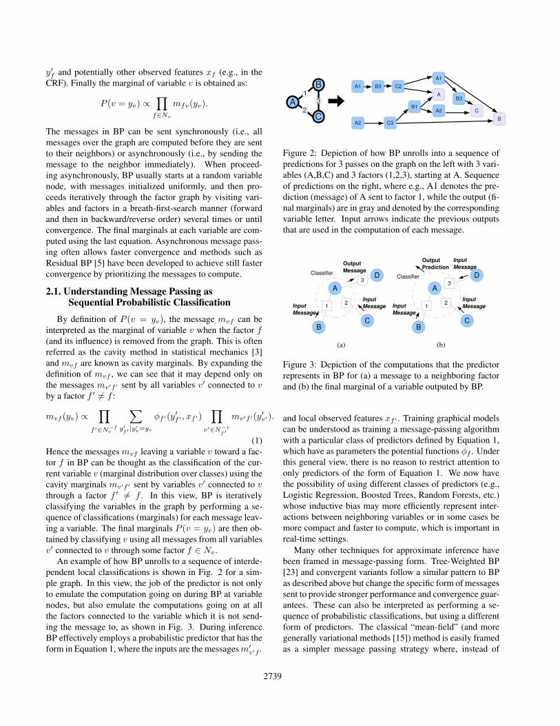
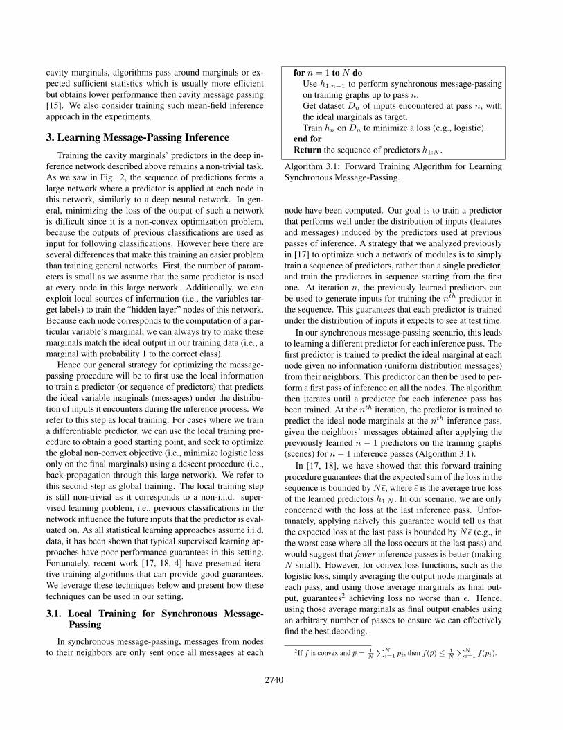
An example of how BP unrolls to a sequence of interde-pendent local classifications is shown in Fig. 2 for a sim-ple graph. In this view, the job of the predictor is not onlyto emulate the computation going on during BP at variablenodes, but also emulate the computations going on at allthe factors connected to the variable which it is not send-ing the message to, as shown in Fig. 3. During inferenceBP effectively employs a probabilistic predictor that has theform in Equation 1, where the inputs are the messagesm′v′f ′

   

A

B

C

1

23

A1

A2

B3 C2

C3

B1

A1

A2

AB3

B

C

Figure 2: Depiction of how BP unrolls into a sequence ofpredictions for 3 passes on the graph on the left with 3 vari-ables (A,B,C) and 3 factors (1,2,3), starting at A. Sequenceof predictions on the right, where e.g., A1 denotes the pre-diction (message) of A sent to factor 1, while the output (fi-nal marginals) are in gray and denoted by the correspondingvariable letter. Input arrows indicate the previous outputsthat are used in the computation of each message.

Input Message

A

B

D

C

1 2

3Classifier

Input Message

Output Message

(a)

Input Message

A

B

D

C

1 2

3Classifier

Input Message

Input Message

Output Prediction

(b)

Figure 3: Depiction of the computations that the predictorrepresents in BP for (a) a message to a neighboring factorand (b) the final marginal of a variable outputed by BP.

and local observed features xf ′ . Training graphical modelscan be understood as training a message-passing algorithmwith a particular class of predictors defined by Equation 1,which have as parameters the potential functions φf . Underthis general view, there is no reason to restrict attention toonly predictors of the form of Equation 1. We now havethe possibility of using different classes of predictors (e.g.,Logistic Regression, Boosted Trees, Random Forests, etc.)whose inductive bias may more efficiently represent inter-actions between neighboring variables or in some cases bemore compact and faster to compute, which is important inreal-time settings.

Many other techniques for approximate inference havebeen framed in message-passing form. Tree-Weighted BP[23] and convergent variants follow a similar pattern to BPas described above but change the specific form of messagessent to provide stronger performance and convergence guar-antees. These can also be interpreted as performing a se-quence of probabilistic classifications, but using a differentform of predictors. The classical “mean-field” (and moregenerally variational methods [15]) method is easily framedas a simpler message passing strategy where, instead of

2739

cavity marginals, algorithms pass around marginals or ex-pected sufficient statistics which is usually more efficientbut obtains lower performance then cavity message passing[15]. We also consider training such mean-field inferenceapproach in the experiments.

3. Learning Message-Passing InferenceTraining the cavity marginals’ predictors in the deep in-

ference network described above remains a non-trivial task.As we saw in Fig. 2, the sequence of predictions forms alarge network where a predictor is applied at each node inthis network, similarly to a deep neural network. In gen-eral, minimizing the loss of the output of such a networkis difficult since it is a non-convex optimization problem,because the outputs of previous classifications are used asinput for following classifications. However here there areseveral differences that make this training an easier problemthan training general networks. First, the number of param-eters is small as we assume that the same predictor is usedat every node in this large network. Additionally, we canexploit local sources of information (i.e., the variables tar-get labels) to train the “hidden layer” nodes of this network.Because each node corresponds to the computation of a par-ticular variable’s marginal, we can always try to make thesemarginals match the ideal output in our training data (i.e., amarginal with probability 1 to the correct class).

Hence our general strategy for optimizing the message-passing procedure will be to first use the local informationto train a predictor (or sequence of predictors) that predictsthe ideal variable marginals (messages) under the distribu-tion of inputs it encounters during the inference process. Werefer to this step as local training. For cases where we traina differentiable predictor, we can use the local training pro-cedure to obtain a good starting point, and seek to optimizethe global non-convex objective (i.e., minimize logistic lossonly on the final marginals) using a descent procedure (i.e.,back-propagation through this large network). We refer tothis second step as global training. The local training stepis still non-trivial as it corresponds to a non-i.i.d. super-vised learning problem, i.e., previous classifications in thenetwork influence the future inputs that the predictor is eval-uated on. As all statistical learning approaches assume i.i.d.data, it has been shown that typical supervised learning ap-proaches have poor performance guarantees in this setting.Fortunately, recent work [17, 18, 4] have presented itera-tive training algorithms that can provide good guarantees.We leverage these techniques below and present how thesetechniques can be used in our setting.

3.1. Local Training for Synchronous Message-Passing

In synchronous message-passing, messages from nodesto their neighbors are only sent once all messages at each

for n = 1 to N doUse h1:n−1 to perform synchronous message-passingon training graphs up to pass n.Get dataset Dn of inputs encountered at pass n, withthe ideal marginals as target.Train hn on Dn to minimize a loss (e.g., logistic).

end forReturn the sequence of predictors h1:N .

Algorithm 3.1: Forward Training Algorithm for LearningSynchronous Message-Passing.

node have been computed. Our goal is to train a predictorthat performs well under the distribution of inputs (featuresand messages) induced by the predictors used at previouspasses of inference. A strategy that we analyzed previouslyin [17] to optimize such a network of modules is to simplytrain a sequence of predictors, rather than a single predictor,and train the predictors in sequence starting from the firstone. At iteration n, the previously learned predictors canbe used to generate inputs for training the nth predictor inthe sequence. This guarantees that each predictor is trainedunder the distribution of inputs it expects to see at test time.

In our synchronous message-passing scenario, this leadsto learning a different predictor for each inference pass. Thefirst predictor is trained to predict the ideal marginal at eachnode given no information (uniform distribution messages)from their neighbors. This predictor can then be used to per-form a first pass of inference on all the nodes. The algorithmthen iterates until a predictor for each inference pass hasbeen trained. At the nth iteration, the predictor is trained topredict the ideal node marginals at the nth inference pass,given the neighbors’ messages obtained after applying thepreviously learned n − 1 predictors on the training graphs(scenes) for n− 1 inference passes (Algorithm 3.1).

In [17, 18], we have showed that this forward trainingprocedure guarantees that the expected sum of the loss in thesequence is bounded byNε, where ε is the average true lossof the learned predictors h1:N . In our scenario, we are onlyconcerned with the loss at the last inference pass. Unfor-tunately, applying naively this guarantee would tell us thatthe expected loss at the last pass is bounded by Nε (e.g., inthe worst case where all the loss occurs at the last pass) andwould suggest that fewer inference passes is better (makingN small). However, for convex loss functions, such as thelogistic loss, simply averaging the output node marginals ateach pass, and using those average marginals as final out-put, guarantees2 achieving loss no worse than ε. Hence,using those average marginals as final output enables usingan arbitrary number of passes to ensure we can effectivelyfind the best decoding.

2If f is convex and p = 1N

PNi=1 pi, then f(p) ≤ 1

N

PNi=1 f(pi).

2740

Some recent work is related to our approach. [19]demonstrates that constrained simple classification can pro-vide good performance in NLP applications. The techniqueof [21] can be understood as using forward training on asynchronous message passing using only marginals, simi-lar to mean-field inference. Similarly, from our point ofview, [13] implements a ”half-pass” of hierarchical mean-field message passing by descending once down a hierarchymaking contextual predictions. We demonstrate in our ex-periments the benefits of enabling more general (BP-style)message passing.

3.2. Local Training for Asynchronous Message-Passing

In asynchronous message-passing, messages from nodesto their neighbors are sent immediately. This creates a longsequence of dependent messages that grows with the num-ber of nodes, in addition to the number of inference passes.Hence the previous forward training procedure is imprac-tical in this case for large graphs, as it requires training alarge number of predictors. Fortunately, an iterative ap-proach called Dataset Aggregation (DAgger) [18] that wedeveloped in prior work can train a single predictor to pro-duce all predictions in the sequence and still guaranteesgood performance on its induced distribution of inputs overthe sequence. For our asynchronous message-passing set-ting, DAgger proceeds as follows. Initially inference is per-formed on the training graphs by using the ideal marginalsfrom the training data to classify each node and generatea first training distribution of inputs. The dataset of inputsencountered during inference and target ideal marginals ateach node is used to learn a first predictor. Then the processkeeps iterating by using the previously learned predictor toperform inference on the training graphs and generate a newdataset of encountered inputs during inference, with the as-sociated ideal marginals. This new dataset is aggregatedto the previous one and a new predictor is trained on thisaggregated dataset (i.e., containing all data collected so farover all iterations of the algorithm). This algorithm is sum-marized in Algorithm 3.2. [18] showed that for stronglyconvex losses, such as regularized logistic loss, this algo-rithm has the following guarantee:

Theorem 3.1. [18] There exists a predictor hn in the se-quence h1:N such that Ex∼dhn

[`(x, hn)] ≤ ε + O( 1N ), for

ε = argminh∈H1N

∑Ni=1 Ex∼dhi

[`(x, h)].

dh is the inputs distribution induced by predictor h. Thistheorem indicates that DAgger guarantees a predictor that,when used during inference, performs nearly as well aswhen classifying the aggregate dataset. Again, in our casewe can average the predictions made at each node over theinference passes to guarantee such final predictions wouldhave an average loss bounded by ε + O( 1

N ). To make the

Initialize D0 ← ∅, h0 to return the ideal marginal on anyvariable v in the training graph.for n = 1 to N do

Use hn−1 to perform asynchonous message-passinginference on training graphs.Get datasetD′n of inputs encountered during inference,with their ideal marginal as target.Aggregate dataset: Dn = Dn−1 ∪D′n.Train hn on Dn to minimize a loss (e.g., logistic).

end forReturn best hn on training or validation graphs.

Algorithm 3.2: DAgger Algorithm for Learning Asyn-chronous Message-Passing.

factor O( 1N ) negligible when looking at the sum of loss over

the whole graph, we can choose N to be on the order of thenumber of nodes in a graph. Though in practice, often muchsmaller number of iterations (N ∈ [10, 20]), is sufficient toobtain good predictors under their induced distributions.

3.3. Global Training via Back-Propagation

In both synchronous and asynchronous approaches, thelocal training procedures provide rigorous performancebounds on the loss of the final predictions; however, theydo not optimize it directly. If the predictors learned aredifferentiable functions, a procedure like back-propagation[12] make it possible to identify local optima of the objec-tive (minimizing loss of the final marginals). As this op-timization problem is non-convex and there are potentiallymany local minima, it can be crucial to initialize this de-scent procedure with a good starting point. The forwardtraining and DAgger algorithms provide such an initial-ization. In our setting, Back-Propagation effectively usesthe current predictor (or sequence of) to do inference on atraining graph (forward propagation); then errors are back-propagated through the network of classification by rewind-ing the inference, successively computing derivatives of theoutput error with respect to parameters and input messages.

4. Experiments: Scene LabelingTo demonstrate the efficacy of our approach, we com-

pared our performance to state-of-the-art algorithms on twolabeling problems from publicly available datasets: (1) 3Dpoint cloud classification from a laser scanner and (2) 3Dsurface layout estimation from a single image.

4.1. Datasets

3D Point Cloud Classification. We evaluate on the 3Dpoint cloud dataset3 used in [14]. This dataset consists of17 full 3D laser scans (total of ∼1.6 million 3D points) of

3http://www.cs.cmu.edu/˜ vmr/datasets/oakland 3d/cvpr09/

2741

an outdoor environment and contains 5 object labels: Build-ing, Ground, Poles/Tree-Trunks, Vegetation, and Wires (seeFig. 1). We design our graph structure as in [14] and use thesame features. The graph is constructed by linking each 3Dpoint to its 5 nearest neighbors (in 3D space) and defininghigh-order cliques (clusters) over regions from two k-meansclusterings over points. The features describe the local ge-ometry around a point or cluster (linear, planar or scatteredstructure; and its orientation); as well as a 2.5-D elevationmap. In [14], performance is evaluated on one fold whereone scene is used for training, one for validation, and theremaining 15 are used for testing. In order to allow eachmethod to better generalize across different scenes, we in-stead split the dataset into 2 folds with each fold containing8 scans for testing and the remaining 9 scans are used fortraining and validation (we always keep the original train-ing scan in both folds’ training sets). We report overall per-formances on the 16 test scans.

3D Surface Layout Estimation. We also evaluate ourapproach on the problem of estimating the 3D surfacelayout from single images, using the Geometric ContextDataset4 from Hoiem et al. [7]. In this dataset, the prob-lem is to assign the 3D geometric surface labels to pixels inthe image (see Fig. 1). This task can be viewed as a 3-classor 7-class labeling problem. In the 3-class case, the labelsare Ground/Supporting Surface, Sky, and Vertical structures(objects standing on the ground), and in the 7-class casethe Vertical class is broken down into 5 subclasses: Left-perspective, Center-perspective, Right-perspective, Porous,and Solid. We consider the 7-class problem. In [7] the au-thors use superpixels as the basic entities to label in con-junction with 15 image segmentations. Various featuresare computed over the regions which capture location andshape, color, texture, and perspective. Boosted decisiontrees are trained per segmentation and are combined to ob-tain the final labeling. In our approach, we define a graphover the superpixels, create edges between adjacent super-pixels, and consider the multiple segmentations as high-order cliques. We use the same respective features and 5-fold evaluation as detailed in [7].

4.2. Approaches

Conditional Random Field (CRF). One baseline is apairwise, Pott’s CRF, trained using asynchronous Loopy BPto estimate the gradient of the partition function.

Max-Margin Markov Network (M3N). Another is thehigh-order [8], associative M3N [20] model from [14]; weuse their implementation5. We analyzed linear models op-timized with the parametric subgradient method (M3N-P)and with functional subgradient boosting (M3N-F).

Synchronous Mean-Field Inference Machine. We

4http://www.cs.illinois.edu/homes/dhoiem/projects/data.html5http://www-2.cs.cmu.edu/˜ vmr/software/software.html

used our proposed approach to train a synchronous mean-field inference machine (MFIM) using the forward trainingprocedure (Sect. 3.1). A simple logistic regressor is usedto predict the node marginals (messages) at each pass. Asthis is a mean-field approach, at each node we predict a newmarginal using all of its neighbors’ messages (i.e., no cavitymethod). For the 3D point cloud dataset, the feature vec-tors are obtained by concatenating6 the messages with thenode, edge, and cluster 3D features. For 3D surface estima-tion, we defined the feature vectors similarly except that theedge/cluster features are averaged together instead of beingconcatenated.

Asynchronous BP Inference Machine. We also trainan asynchronous belief propagation inference machine. Inthis case, inference starts at a random node and proceedsin breadth-first-search order and alternates between forwardand backward order at consecutive passes. Again a sim-ple logistic regressor to predict the node marginals (mes-sages). We compare 3 different approaches for optimizingit. BPIM-D: DAgger7 from Sect. 3.2. BPIM-B: Back-Propagation starting from a 0 weight vector. BPIM-DB:Back-Propagation starting from the predictor found withDAgger (only for point cloud dataset). For both datasets,the input feature vector is constructed exactly as for the syn-chronous mean-field inference machine when predicting thefinal classification of a node. However, when sending mes-sages to neighbors and clusters the cavity method is used(i.e., the features related to the node/cluster we are sendinga message to are removed from the concatenation/average).

4.3. Results

We measure the performance of each method in termsof per site (i.e., over points in the point cloud and super-pixels in the image) accuracy, the Macro-F1 score (averageof the per class F1 scores), and Micro-F1 score (weightedaverage, according to class frequency, of the per class F1scores). Table 1 summarizes the results for each approachand dataset.

3D Point Cloud Classification. We observe that thebest approach overall is the functional gradient M3N ap-proach of [14]. We believe that for this particular datasetthis is due to the use of a functional gradient method, whichis less affected by the scaling of features and large classimbalance in this dataset. We can observe that when us-ing the regular parametric subgradient M3N approach, theperformance is slightly worse than our inference machineapproach, also optimized via parametric gradient descent.Hence using a functional gradient approach when training

6We concatenate up to 20 neighbors, ordered by physical distance, andappend with zeros if there are less than 20 neighbors

7DAgger is used for 30 iterations, and the predictor that has the low-est error rate (from performing message-passing inference) on the trainingscenes is returned as the best one.

2742

3D Point Clouds 3D Surface LayoutAccuracy Macro-F1 Micro-F1 Accuracy Macro-F1 Micro-F1

BPIM-D 0.9795 0.8206 0.9799 0.6467 0.5971 0.6392BPIM-B 0.9728 0.6504 0.9706 0.6287 0.5705 0.6149

BPIM-DB 0.9807 0.8305 0.9811 - - -MFIM 0.9807 0.8355 0.9811 0.6378 0.5947 0.6328CRF 0.9750 0.8067 0.9751 0.6126 0.5369 0.5931

M3N-F 0.9846 0.8467 0.9850 0.6029 0.5541 0.6001M3N-P 0.9803 0.8230 0.9806 - - -

[7] - - - 0.6424 0.6057 0.6401

Table 1: Comparisons of overall performances on the two datasets.

1 2 3 4 5 6 7 80.015

0.02

0.025

0.03

0.035

0.04

Inference Pass

Test

Erro

r

CRF

BPIM−B

BPIM−D

BPIM−DB

MFIM

Figure 4: Average test error as a function of pass for eachmessage-passing method on the 3D classification task.

the base predictor with our inference machine approachescould potentially lead to improved performance. Both infer-ence machines (MFIM, BPIM-D) outperform the baselineCRF message-passing approach. Additionally, we observethat using backpropagation on the output of DAgger slightlyimproved performance. Without this initialization, back-propagation does not find a good solution. In this particulardataset we do not notice any advantage of the cavity method(BPIM-D) over the mean-field approach (MFIM). In Fig.4, we observe that the error of all asynchronous message-passing approaches converge roughly after 3-4 inferencepasses, while the synchronous message-passing (MFIM)converges slightly slower and requires around 6 passes.

We also performed the experiment on the smaller splitused in [14] (i.e., training on a single scene) and ourapproach (BPIM-D) obtained slightly better accuracy of97.27% than the best approach in [14] (M3N-F: 97.2%).However, in this case, backpropagation did not further im-prove the solution on the test scenes as it overfits more to asingle training scene.

3D Surface Layout Estimation. In this experiment ourBPIM-D approach performs slightly better than all other ap-proaches in terms of accuracy, including the performanceof the previous state-of-the-art in [7]. In terms of F1 score,

[7] is slightly better. Given that [7] used a more power-ful base predictor (boosted trees) than our logistic regres-sor, we believe we could also achieve better performanceusing more complex predictors. We notice here a larger dif-ference between the BPIM and MFIM approaches, whichconfirms the cavity method can lead to better performance.Here the M3N-F approach did not fare very well and allmessage-passing approaches outperformed it. All inferencemachine approaches also outperformed the baseline CRF.Fig. 6 shows a visual comparison of the M3N-F, MFIM,BPIM-D and [7] approaches on two test images. The out-puts of BPIM-D and [7] are very similar, but we can observemore significant improvements over the M3N-F.

5. Conclusion and Future Work

We presented a novel approach to structured predictionwhich is simple to implement, has strong performance guar-antees, and performs as well as state-of-the-art methodsacross multiple domains. The efforts presented here byno means represent the end of a line of research; we be-lieve there is substantial remaining research to be done inlearning inference machines. In particular, while we presentsimple effective approaches (Forward training, DAgger) forleveraging local information to learn a deep modular infer-ence machine, we believe alternate techniques may be veryeffective at addressing this optimization. Further, whilethe message passing approaches we investigate here oftenprovide outstanding performance, other methods includingsampling and graph-cut based approaches are often consid-ered state-of-the-art for other tasks. We believe the simi-lar ideas of unrolling such procedures and using notions ofglobal and local training may prove equally effective andare worthy of investigation. Additionally, a significant (un-explored) benefit of the approach taken here is that we caneasily include features and computations not typically con-sidered as part of the graphical model approach and stillattempt to optimize overall performance; e.g., computingnew features or changing the structure based on the resultsof partial inference.

2743

Figure 5: Estimated 3D geometric surface layouts. From left to right: M3N-F, Hoeim et al. [7], BPIM-D, Ground truth.

Figure 6: Estimated 3D point cloud labels. From left to right: M3N-F, M3N-P, MFIM, Ground truth.

Acknowledgements

This work is supported by the ONR MURI grantN00014-09-1-1052, Reasoning in Reduced InformationSpaces, by the National Sciences and Engineering ResearchCouncil of Canada (NSERC), and by a QinetiQ NorthAmerica Robotics Fellowship.

References[1] Y. Bengio. Learning deep architectures for AI. Foundations and

Trends in Machine Learning, 2(1), 2009.[2] Y. Boykov, O. Veksler, and R. Zabih. Fast approximate energy mini-

mization via graph cuts. T-PAMI, 23(1), 1999.[3] L. Csato, M. Opper, and O. Winther. Tap gibbs free energy, belief

propagation and sparsity. In NIPS, 2001.[4] H. Daume III, J. Langford, and D. Marcu. Search-based structured

prediction. MLJ, 75(3), 2009.[5] G. Elidan, I. McGraw, and D. Koller. Residual belief propagation: In-

formed scheduling for asynchronous message passing. In UAI, 2006.[6] T. Finley and T. Joachims. Training structural svms when exact in-

ference is intractable. In ICML, 2008.[7] D. Hoiem, A. A. Efros, and M. Hebert. Recovering surface layout

from an image. IJCV, 75(1), 2007.[8] P. Kohli, L. Ladicky, and P. H. Torr. Robust higher order potentials

for enforcing label consistency. IJCV, 82(3), 2009.[9] A. Kulesza and F. Pereira. Structured learning with approximate in-

ference. In NIPS, 2008.[10] S. Kumar, J. August, and M. Hebert. Exploiting inference for ap-

proximate parameter learning in discriminative fields: An empiricalstudy. In EMMCVPR, 2005.

[11] J. Lafferty, A. McCallum, and F. Pereira. Conditional random fields:Probabilistic models for segmenting and labeling sequence data. InICML, 2001.

[12] Y. LeCun, L. Bottou, Y. Bengio, and P. Haffner. Gradient-basedlearning applied to document recognition. IEEE, 86(11), 1998.

[13] D. Munoz, J. A. Bagnell, and M. Hebert. Stacked hierarchical label-ing. In ECCV, 2010.

[14] D. Munoz, J. A. Bagnell, N. Vandapel, and M. Hebert. Contex-tual classification with functional max-margin markov networks. InCVPR, 2009.

[15] M. Opper and D. Saad. Advanced Mean Field methods – Theory andPractice. MIT Press, 2000.

[16] J. Pearl. Probabilistic Reasoning in Intelligent Systems: Networks ofPlausible Inference. Morgan Kaufmann Publishers Inc., 1988.

[17] S. Ross and J. A. Bagnell. Efficient reductions for imitation learning.In AISTATS, 2010.

[18] S. Ross, G. J. Gordon, and J. A. Bagnell. No-Regret Reductions forImitation Learning and Structured Prediction. In AISTATS, 2011.

[19] D. Roth, K. Small, and I. Titove. Sequential learning of classifiersfor structured prediction problems. In AISTATS, 2009.

[20] B. Taskar, C. Guestrin, and D. Koller. Max-margin markov networks.In NIPS, 2003.

[21] Z. Tu and X. Bai. Auto-context and its application to high-level vi-sion tasks and 3d brain image segmentation. T-PAMI, 32(5), 2009.

[22] M. J. Wainwright. Estimating the “wrong” graphical model: Benefitsin the computation-limited setting. JMLR, 7(11), 2006.

[23] M. J. Wainwright, T. Jaakkola, and A. S. Willsky. Tree-based repa-rameterization for approximate estimation on loopy graphs. In NIPS,2001.

2744