learning objectives : introduce petri nets dynamic behavior modeling of manufacturing systems using...

Learning objectives :• Introduce Petri nets• Dynamic behavior modeling of manufacturing systems using PN• Analysis of Petri net models

Textbook :

J.-M. Proth and X. Xie, Petri nets: a tool for design and management of manufacturing systems, John Wiley & Sons, 1996

C. Cassandras and S. Lafortune, Introduction to Discrete Event Systems, Springer, 2007

Chapter 3Petri nets

1

Plan

• Introduction to Petri nets

• Formal definitions

• Petri net models of manufacturing system

• Elementary classes of Petri nets

• Properties of PN models

• Analysis methods

22

33

Introduction to Petri nets

A two-product system

4

• Two types P1 and P2 of products are produced.

• The production of each product requires two operations.

• The first operation is performed by a shared machine.

• The second operation is performed by a dedicated machine.

• There is at most one product of each type loaded in the system at any time.

• When a product finishes, a new product of the same type is dispatched.

To be modelled using an usual process-resource modelling approach.

A two-product systemProcess modeling

5

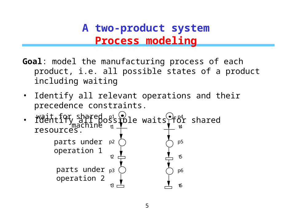
Goal: model the manufacturing process of each product, i.e. all possible states of a product including waiting

• Identify all relevant operations and their precedence constraints.

• Identify all possible waits for shared resources.

p1

t1

p2

t2

p3

t3

p4

t4

p5

t5

p6

t6

wait for shared machine

parts under operation 1


A two-product systemProcess modelling

6

• Goal: model the manufacturing process of each product.

• Include eventual constraints related to production control.

p1

t1

p2

t2

p3

t3

p4

t4

p5

t5

p6

t6

A two-product systemResource modelling

7

• Goal: modelling resource contraint + eventual priority constraints

p1

t1

p2

t2

p3

t3

p4

t4

p5

t5

p6

t6

p7

Identifies

•transitions after which the resource is first needed

•transitions after which the resource is no longer needed

Places and transitions

• A PETRI NET is a bipartite graph which consists of two types of nodes: places and transitions connected by directed arcs.

• Place = circle, transition = bar or box.

• An arc connects a place to a transition or a transition to a place.

• No arcs between nodes of the same type.

• Input and output places of a transition

• Input and output transitions of a place

p1

p2

p3

p4

p5 t1

t2

t3

t4

t5

Token and markingsystem state

Each place contains a number of tokens. The distribution of tokens in the Petri net is called the marking. Representations of a marking:•a vector M = (m1, m2, …, mn) where mi = nb of tokens in place pi•a multi-set such as M = p1 2p3 The marking of an PN = state of the corresponding system. The initial state of the system = the initial marking, denoted as M0.

Example: M = ( ???) = ??? 9

p1

p2

p3

p4

p5 t1

t2

t3

t4

t5

System dynamics by transition firing

• A transition is said enabled (firable) if each of its input places contains at least one token. An enabled transition can fire.

• Firing a transition removes a token from each input place and add one token to each ouput place.

• Firing a transition leads to a new marking that enables other transitions.

• The dynamic behavior of the corresponding system = evolution of the marking and transition firings

• Convention: simultaneous transition firings are forbidden. 10

Sequence of transitions

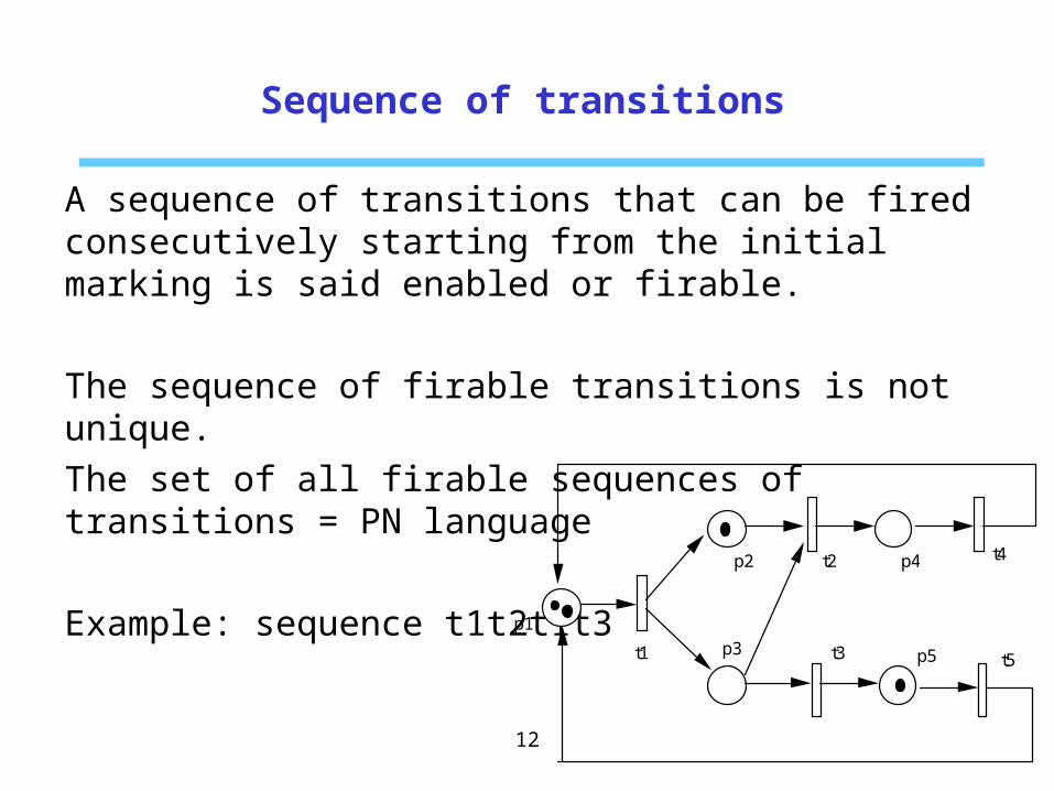
A sequence of transitions that can be fired consecutively starting from the initial marking is said enabled or firable.

The sequence of firable transitions is not unique.

The set of all firable sequences of transitions = PN language

Example: sequence t1t2t1t3

12

p1

p2

p3

p4

p5 t1

t2

t3

t4

t5

Formal definitions

13

Petri Nets

A Petri net is a five-tuple PN = (P, T, A, W, M0) where:P = { p1, p2, ..., pn} is a finite set of placesT = { t1, t2, ..., tm } is a finite set of transitions A (P×T) (T×P) is a set of arcsW : A → { 1, 2, ... } is a weight functionM0 : P → { 0, 1, 2, ... } is the initial markingP T = and P T =

PN without the initial marking is denoted by N:N = (P, T, A, W)PN = (N, M0)

A Petri net is said ordinary if w(a) = 1, a A.14

Graphic representation

Similar to that of ordinary PN but with default weight of 1 when not explicitly represented.

15

p1

p2

p3

p4

p5 t1

t2

t3

t4

t5

2

Transition firing

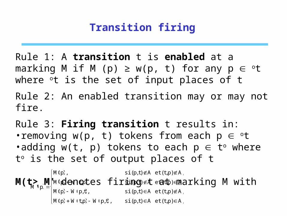
Rule 1: A transition t is enabled at a marking M if M (p) ≥ w(p, t) for any p ot where ot is the set of input places of t

Rule 2: An enabled transition may or may not fire.

Rule 3: Firing transition t results in:•removing w(p, t) tokens from each p ot•adding w(t, p) tokens to each p to where to is the set of output places of t

M(t> M' denotes firing t at marking M with

M' p

M p , si (p, t) A et ( t,p) A,

M p W t,p , si (p, t) A et ( t,p) A,

M p W p,t , si (p, t) A et ( t,p) A,

M p W t,p W p,t , si (p, t) A et ( t,p) A,

Transition firing

17

2 2 2 2

2

2 2

2

Basic concepts

Source transition: transition without input places, i.e. ot = .

Sink transition: transition without output places, i.e. to = .

Source place: place without input transitions, i.e. op = .

Sink place: place without output transitions, i.e. po = .

Self-loop: a couple (p, t) such that t is both input and output transition of p

Path: a sequence of nodes s1s2…sn such that si+1 is an output node of si.

Circuit: a path such that sn = s1.

Online illustration

Incidence matrices

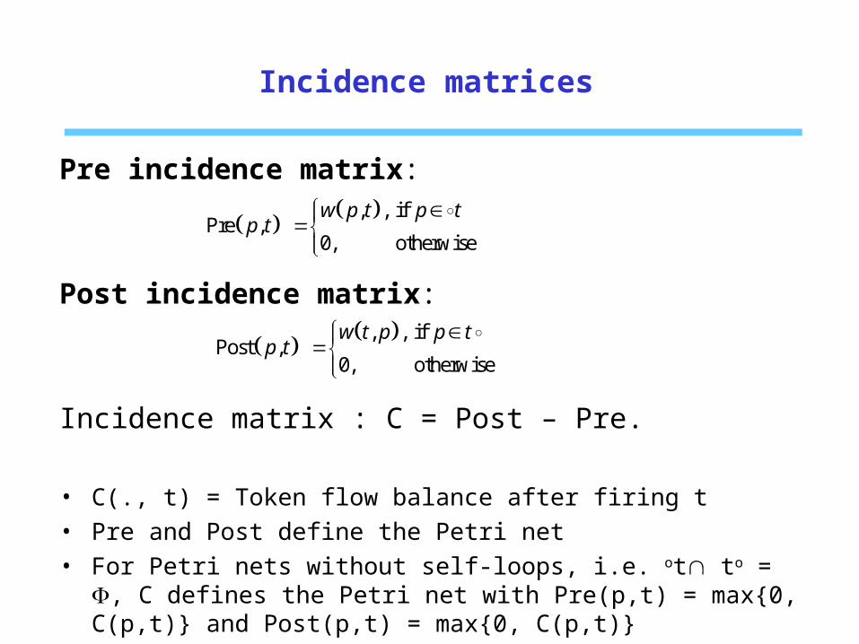
Pre incidence matrix:

Post incidence matrix:

Incidence matrix : C = Post – Pre.

• C(., t) = Token flow balance after firing t

• Pre and Post define the Petri net

• For Petri nets without self-loops, i.e. ot to = , C defines the Petri net with Pre(p,t) = max{0, C(p,t)} and Post(p,t) = max{0, C(p,t)}

, , ifPre ,

0, otherwise

w p t p tp t

, , ifPost ,

0, otherwise

w t p p tp t

Incidence matrices

Example:

Pre = ???, Post = ???, C = ???

p1

p2

p3

p4

p5 t1

t2

t3

t4

t5

2

Incidence matrices

Enabled transition: A transition t is enabled at a marking M if

M ≥ Pre(●, t)

Transition firing: Firing a transition t at marking M leads to

M’ = M + C(●, t)

Sequence of transitions: Firing a sequence = t1t2…tn of transition starting from marking M leads to:

where is the counting vector of the sequence . (proof) Equation (1) is also called « state equation ».

Question: can this equation be used to checked the feasibility of a sequence and the reachability of a marking?

' (1)M M C

Incidence matrices

Example:

Markings after = t1t5t2t3t5

p1

p2

p3

p4

p5 t1

t2

t3

t4

t5

2

Petri net models of manufacturing systems

PN models of key characteristics

Precedence relation:

24

start Activity1 Activity2 End

Alternattive process Start End

Alternative processes:

Parallel processes:

Start parallel process

End

Synchronization: Waiting

Sync


Buffer of finite capacity (4):

25

FIFO system:

Part arrival

Part request

pv

pb


26

Shared resources:

Process with Resource Waiting for

Resource

Other Activities

r

p1

p2


27

Dedicated machine:

Shared machine:


28

Assembly operation: Unreliable machines:

n

1

n 2

Input buffer

output buffer capacity

pf

pw pb

pr

A robotic cell

29

M 1

M 2

S

Robot

t 1 M 1

t 2 Unload

R Stock n Q

load t 3

t 4

P 2

M 2

T

P 1

Z 1

Z 2

I

O

A two-product system

30

• Two types P1 and P2 of products are produced.

• The production of each product requires two operations.

• The first operation is performed by a shared machine.

• The second operation is performed by a dedicated machine.

• There is at most one product of each type loaded in the system at any time.

• When a product finishes, a new product of the same type is dispatched.

To be modelled using an usual process-resource modelling approach.

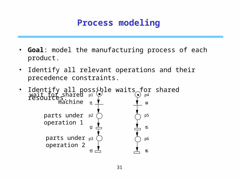
Process modeling

31


• Identify all relevant operations and their precedence constraints.

• Identify all possible waits for shared resources.

p1

t1

p2

t2

p3

t3

p4

t4

p5

t5

p6

t6

wait for shared machine



Process modelling

32


• Include eventual constraints related to production control.

p1

t1

p2

t2

p3

t3

p4

t4

p5

t5

p6

t6

Resource modelling

33

• Goal: modelling resource contraint.

p1

t1

p2

t2

p3

t3

p4

t4

p5

t5

p6

t6

p7

Identifies

•transitions after which the resource is first needed

•transitions after which the resource is no longer needed

Elementary classes of Petri nets

34

Pure Petri nets

Definition: A Petri net free of self loop is said pure, i.e. ot to = .

Theorem : All impure Petri nets can be transformed into pure Petri nets.

35

p1

p2

t1

t2

p1

p2 p0

b1

e1

b2

e2

Ordinary Petri nets

STATE MACHINESEach transition has exactly one input place and one output place. Property: The total number of token is constant.

EVENT GRAPHS (OR MARKED GRAPHS)Each place has exactly one input and one output transition.

Property: The total number of tokens in each elementary circuit is constant

36

p1

p2 p3

t1 t2

t3 t4

Ordinary Petri nets

FREE-CHOICE NETScard(p°) > 1 °(p°) = {p}, p P.

Property : For any free-choice net, a t' in conflict with an enalbed transition t , i.e. •t' •t ≠ , is also enabled.

EXTENDED FREE-CHOICE NETS p1°p2° ≠ p1° = p2°, p1, p2 P

An extended free-choice net can always be transformed into a free-choice net.

37

Ordinary Petri nets

ASYMMETRIC CHOICE NETSp1°p2° ≠ p1° p2° or p2° p1° , p1, p2 P

Theorem : For any asymmetric choice net, the set {p1, p2, …, pk} of input places of any transition can be renumbered such that p1° p2° … pk°.

38

r

p1

p2

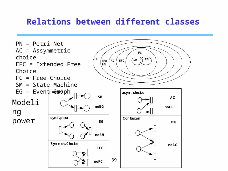
Relations between different classes

39

SM EG

FC

EFC AC Ord. PN

PN

PN = Petri NetAC = Assymmetric choiceEFC = Extended Free ChoiceFC = Free ChoiceSM = State MachineEG = Event Graph

SM

noEG

Conflict

sync. para. EG

noSM

Symmet. Choice EFC

noFC

AC

noEFC

asym. choice

Confusion PN

noAC

Modeling power

Properties of PN models

40

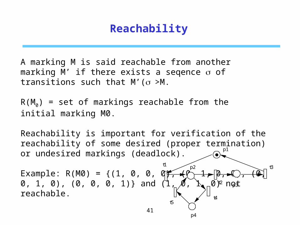
Reachability

A marking M is said reachable from another marking M’ if there exists a seqence of transitions such that M’(>M. R(M0) = set of markings reachable from the initial marking M0. Reachability is important for verification of the reachability of some desired (proper termination) or undesired markings (deadlock).

Example: R(M0) = {(1, 0, 0, 0), (0, 1, 0, 0), (0, 0, 1, 0), (0, 0, 0, 1)} and (1, 0, 1, 0) not reachable.

41

p1 :

p2

p3

p4

t1

t2

t3

t4 t5

Reachability

Theorem1 (monotonicity) : Any sequence s of transitions firable starting from a marking M0 is also firable starting from M0’ such that M0' ≥ M0. Theorem2 (necessary condition) : The equation system CY = M - M0 with Y ≥ 0 has a solution for all reachable marking M. Theorem3 (Acyclic PN) : For any PN free of cycles, a marking M is reachable iff the equation system C Y = M - M0 with Y ≥ 0 has a solution.

Ex: Find a PN and a marking that is not reachable but for which condition of Theorem 2 holds.

42

Boundedness

A place p is said k-bounded if the number of tokens in p never exceed k, i.e. M(p) ≤ k, M � R(M0). A Petri net is said k-bounded if all places are k-bounded, i.e. M(p) ≤ k, p and M � R(M0). A Petri net is said bounded if it is k-bounded for some k > 0. A Petri net is said safe if it is 1-bounded, M(p) ≤ 1, p and M � R(M0). Boundedness is often needed for a well-designed system as, without this property, goods could accumulated without limit, which is often a design error.

43

Boundedness

44

p

p

p'

Boundedness

Theorem (monotonicity) : If (N, M0) is bounded, then (N, M0’) such that M0' ≤ M0 is bounded. Theorem (necessary condition) : A Petri net (N, M0) is k-bounded if M(p) ≤ k, p and M such that M = M0 + CY for some Y ≥ 0.

45

Liveness

A transition t is said live if it can always be made enabled starting from any reachable marking, i.e. M � R(M0), M' � R(M) such that M‘(t>. A Petri net is said live if all transitions are live.

A transition is said quasi live if it can be fired at least once, i.e. M � R(M0) such that M(t>.

A Petri net is said quasi live if all transitions are quasi live.

A marking M is said a deadlock or dead marking if no transition is enabled at M.

A Petri net is said deadlock-free if it does not contain any deadlock.

46

Liveness

• Liveness implies the absence of total or partial deadlock and is often required for well-designed systems. But the reverse is not true.

• Deadlock often results from resource sharing and synchronization of parallel processes.

• No monotonicity of liveness as the Petri net below is not live if M0(R1) = 0, live if M0(R1) = 1, and not live if M0(R1) = 2.

47

S1 S2 R1

R2 R3

S1 S2 R1

R2 R3 PN1 PN2

Reversibility

A Petri net (N, M0) is said reversible if the initial marking remains reachable from any reachable marking, i.e. M0 R(M), � M R(M0)� A marking M* is said a home state if it is reachable from all reachable markings, i.e. M* R(M), � M R(M0) .� Existence of the reversibility ensures that the system can always recover the normal behavior and is important for systems subject to failures.

Existence of home state is important for systems requiring proper termination.

Reversiblity implies existence of home states but the reverse is not true.

48

Reversibility

49

p1

p2 :

p3

p4

t1

t2

t3

t4 t5

p5: mach free but not usable

t4

p1

p2

p3

p4

t1

t2

t3

t4 t5

p5:

t4

Reversibility, liveness and boundedness are independent

Analysis methods

50

Reachability tree

Definition: The reachability tree, also called marking graph, of a Petri net (N, M0) is a graph in which

•nodes corresponds to reachable markings

•arcs correpond to feasible transitions.

Remark: the reachability tree of an unbounded PN is unlimited.

p1 p2 t1 t2

[0, 1] M0

[0, 0] M1

t2

p1

p2 t1 t2

[1, 1] M0

[0, 2] M1

[2, 0] M2

t1

t2

t2

t1

p1 p2 t1 t2

[0, 0] M0

[0, 1] M1

t1

t2

[0, 2] M2

t1

t2 •••

Coverability tree

Symbol "" implying « as great as possible » with the following properties: > n, ± n = , for all integer n and ≥ .

52

p1 p2 t1 t2

[0, 0] M0

[0, ] M1

t1 • M1 covers M0• Repeat t1 leads to tokens in p2. • Replace M1 by [0, ]

[0, 0] M0

[0, ] M1

t1 [0, ] M1

t1

t2

old

[0, 0] M0

[0, ] M1

t1

t1

t2

new

[0, ] M1

old

Step1

Step2

Step3

Coverability tree

Algorithm of coverability tree

1. Initiate the tree by a root node labeled M0 and marked as "new".

2. While there exists "new" nodes :

2.1. Select a "new" node A. Let M be its marking.

2.2. If there exists a node B with marking M on the path from the root to A, then mark A as "old" and go to 2.

2.3. If M is a dead marking, then mark A"dead-end" and go to 2.

2.4. Otherwise, for each transition t enabled at M,

2.4.1. Add a node C, an arc from A to C with label t, mark C "new".

2.4.2. Determine the marking M’ of node C.

2.4.3. If, on the path from the root to node C, there exists a node D with marking M" such that M' ≥ M" & M'(p) > M"(p) for some p, then M'(p) = for all p such that M'(p) > M"(p).

2.5. Go to 2. 53

Coverability tree

Theorem (boundedness) : A Petri net (N, M0) is bounded iff the symbol does not appear in the coverability tree. Theorem (bounded PN) : For a bounded Petri net, it is deadlock-free iff any node of the reachability tree has a successor. It is reversible iff the reachability tree is strongly connected. A transition t is live iff it appears a all strongly connected components that do not have arcs going out.

Remark: Liveness and reversibility of unbounded PN cannot be checked with coverability trees.

54

Siphons and traps

A siphon is a subset of places such that any input transition of a place is an output transition of some other place.

A trap is a subset of places such that any output transition of a place is an output transition of some other place.

55

Siphon

ifthen

Trap

thenif

Siphons and traps

Theorem: For any ordinary PN,

•A siphon free of tokens at a marking remains token-free

•A trap marked by a marking remains marked

•The empty places of a dead marking form a siphon for any marking such that no transition is enabled.

•A Petri net is deadlock-free if no siphon eventually becomes empty.

56

Siphon

ifthen

Trap

thenif

Siphons and traps

Theorem: A connected event graph (N, M0) is live iff every circuit contains a token. A live event graph is reversible. A connex event graph is bounded iff it is strongly connected.

Theorem: A connected state machine is always bounded. It is live and reversible iff it is strongly connected.

Theorem : A free-choice (extended or not) (N, M0) is live iff all siphon contains a trap marked at M0.

Theorem : An assymetric net (N, M0) is live iff no siphon can become unmarked.

Remarks:

•Whether all siphons remain marked can be checked by integer programming.

•For usual manufacturing systems, both liveness and reversibility are ensured if no siphon can become unmarked

57

Siphons and traps

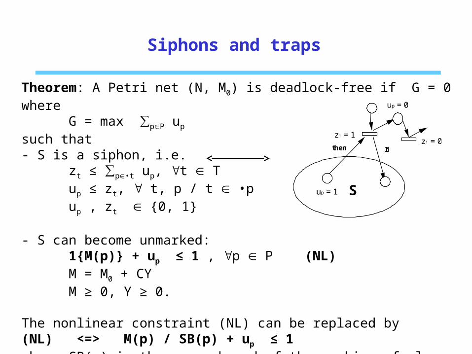
Theorem: A Petri net (N, M0) is deadlock-free if G = 0 where G = max ∑pP� up

such that- S is a siphon, i.e.

zt ≤ ∑p•t� up, t � Tup ≤ zt, t, p / t •p�up , zt � {0, 1}

- S can become unmarked:1{M(p)} + up ≤ 1 , p � P (NL)M = M0 + CY M ≥ 0, Y ≥ 0.

The nonlinear constraint (NL) can be replaced by(NL) <=> M(p) / SB(p) + up ≤ 1where SB(p) is the upper bound of the marking of place p.

S

If then

u p = 0

z t = 1

u p = 1

z t = 0

Siphons and traps

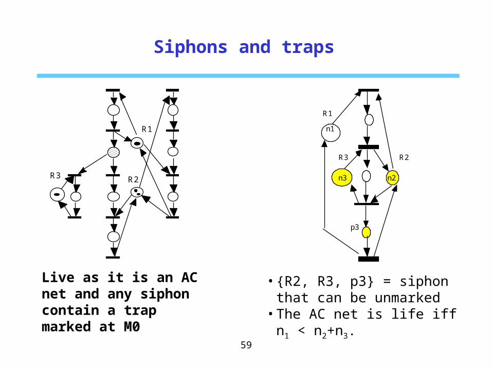
Live as it is an AC net and any siphon contain a trap marked at M0

59

R1

R2 R3

R1

R2 R3

n1

n3 n2

p3

• {R2, R3, p3} = siphon that can be unmarked

• The AC net is life iff n1 < n2+n3.

p-invariants

Definition:

•A integer vector X≥0 of dimension n = |P| is a p-invariant if Xt C = 0.

•The set of places pi with Xi > 0 is called the support of the p-invariant and is denoted ||X||.

•A p-invariant X is said minimal if there does not exist another p-invariant X’ such that X' ≠ X and X' ≤ X.

Exampel:

60

S1 S2 R1

R2 R3

p-invariants

Theorem: X is a p-invariant iff, for all M0, Xt M = Xt M0, M � R(M0).Theorem : Any linear combination of p-invariants is a p-invariant.Theorem : All p-invariant is a non negative linear combination of minimal p-invariants. Remark : For PN models of real systems, a minimal p-invariant has clear physical significance (resource, production control strategies, ...) and can be derived by inspection of resources and processes.

Exampe:

61

S1 S2 R1

R2 R3

t-invariants

Definition:

•A integer vector Y≥0 of dimension m = |T| is a t-invariant if CY = 0.

•The set of transitions ti with Yi > 0 is called the support of the t-invariant and is denoted ||Y||.

•A t-invariant Y is said minimal if there does not exist another t-invariant Y’ such that Y' ≠ Y and Y' ≤ Y.

Exampel:

62

S1 S2 R1

R2 R3

t-invariants

Theorem: Let s be a sequence of transitions tranforming M0 into M and Y its counting vector. Then M = M0 iffY is an t-invariant.Theorem : Any linear combination of t-invariants is a t-invariant.Theorem : All t-invariant is a non negative linear combination of minimal t-invariants. Remark : In general, a minimal t-invariant corresponds to a process that can be repeat for ever. They can be identified by neglecting resources.

Exampe:

63

S1 S2 R1

R2 R3

Structural properties

STRUCTURAL BOUNDEDNESS A Petri net N is structurally bounded if it is bounded starting from any M0.Criterion : N is structurally bounded X > 0, XTC ≤ 0. Theorem: (N, M0) is bounded if it is structurally bounded.

CONSERVATIVENESSA Petri net N is conservative if there exists a vector X > 0 associated with places such that XTM = XTM0, M0, M R(M0).Criterion : N is conservative X > 0, XTC = 0. Theorem: •(N, M0) is bounded if it is conservative.•A Petri net is conservative if all places are covered by some p-invariant.

64


REPETITIVENESSA Petri net N is repetitive if there exists M0 and a feasible firing sequence such that each transition appears infinitely often. Criterion : N is repetitive Y > 0, CY ≥ 0.

Theorem: A live Petri net (N, M0) is repetitive.

CONSISTENCYA Petri net N is consistent if there exist an initial marking M0 and a firing sequence such that > 0 and M0 [ >M0.Criterion : N is consistent Y > 0, CY = 0.

Theorem : •A live Petri net (N, M0) with a home state is consistent.•A live and bounded Petri net (N, M0) is consistent. It is also conservative if it is live and structurally bounded.

65


66

S1 S2 R1

R2 R3

In practice, boundedness reduces to conservativeness.

Consistency and conservativeness provide necessary conditions for liveness and resersibility.

Unfortunately, liveness and resersibility remain difficult to check.

Determination of p- and t-invariants

67

Algorithm of minimal p-invariants1. Set A = In×n with n = |P| and B = C (incidence matrix). Construct matrix [A | B].2. For each transition tj:2.1. Add to [A | B] non negative linear combination of any two lines that zeros the entry of column tj2.2. Remove in the matrix [A | B] all lines i such that the entry (i, j) is not zero.3. p-invariants correspond to lines of matrix A.

The algorithm of t-invariants is similar with C replaced by CT.

2

3

2 2

Topics not addressed in Chapters 2-3

68

Supervisory control with automata theory

Timed Petri nets

Color Petri nets

Petri net controls

Petri net models synthesis

learning objectives : introduce petri nets dynamic behavior modeling of manufacturing systems using...

Documents