1 © J. Fürnkranz

Learning of Rule SetsLearning of Rule Sets

● Introduction Learning Rule Sets Terminology Coverage Spaces

● Separate-and-Conquer Rule Learning Covering algorithm Top-Down Hill-Climbing Rule Evaluation Heuristics Overfitting and Pruning Multi-Class Problems Bottom-Up Hill-Climbing

2 © J. Fürnkranz

Learning Rule SetsLearning Rule Sets

● many datasets cannot be solved with a single rule not even the simple weather dataset they need a rule set for formulating a target theory

● finding a computable generality relation for rule sets is not trivial adding a condition to a rule specializes the theory adding a new rule to a theory generalizes the theory

● practical algorithms use different approaches covering or separate-and-conquer algorithms based on heuristic search

3 © J. Fürnkranz

A sample taskA sample taskTemperature Outlook Humidity Windy Play Golf?

hot sunny high false no hot sunny high true no hot overcast high false yes cool rain normal false yes cool overcast normal true yes mild sunny high false no cool sunny normal false yes mild rain normal false yes mild sunny normal true yes mild overcast high true yes hot overcast normal false yes mild rain high true no cool rain normal true no mild rain high false yes

● Task: Find a rule set that correctly predicts the dependent

variable from the observed variables

4 © J. Fürnkranz

A Simple SolutionA Simple Solution

IF T=hot AND H=high AND O=overcast AND W=false THEN yes IF T=cool AND H=normal AND O=rain AND W=false THEN yes IF T=cool AND H=normal AND O=overcast AND W=true THEN yes IF T=cool AND H=normal AND O=sunny AND W=false THEN yes IF T=mild AND H=normal AND O=rain AND W=false THEN yes IF T=mild AND H=normal AND O=sunny AND W=true THEN yes IF T=mild AND H=high AND O=overcast AND W=true THEN yes IF T=hot AND H=normal AND O=overcast AND W=false THEN yes IF T=mild AND H=high AND O=rain AND W=false THEN yes

● The solution is a set of rules that is complete and consistent on the training examples→ it must be part of the version space

● but it does not generalize to new examples!

5 © J. Fürnkranz

The Need for a BiasThe Need for a Bias

● rule sets can be generalized by generalizing an existing rule (as usual) introducing a new rule (this is new)

● a minimal generalization could be introduce a new rule that covers only the new example

● Thus: The solution on the previous slide will be found as a result of

the FindS algorithm FindG (or Batch-FindG) are less likely to find such a bad

solution because they prefer general theories● But in principle this solution is part of the hypothesis space

and also of the version space⇒ we need a search bias to prevent finding this solution!

6 © J. Fürnkranz

A Better SolutionA Better Solution

IF Outlook = overcast THEN yes

IF Humidity = normal AND Outlook = sunny THEN yes

IF Outlook = rainy AND Windy = false THEN yes

7 © J. Fürnkranz

Recap: Batch-FindRecap: Batch-Find

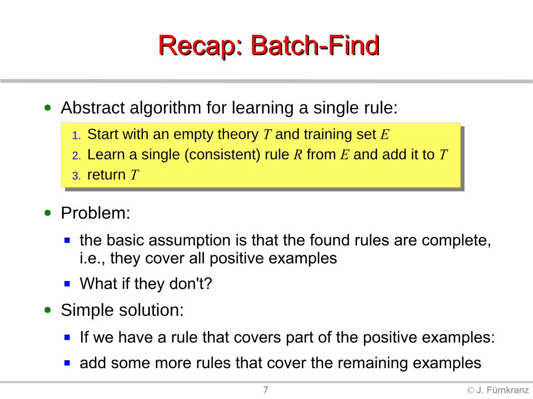
● Abstract algorithm for learning a single rule:

1. Start with an empty theory T and training set E2. Learn a single (consistent) rule R from E and add it to T 3. return T

● Problem: the basic assumption is that the found rules are complete,

i.e., they cover all positive examples What if they don't?

● Simple solution: If we have a rule that covers part of the positive examples: add some more rules that cover the remaining examples

8 © J. Fürnkranz

Separate-and-ConquerSeparate-and-ConquerRule LearningRule Learning

Learn a set of rules, one by one1. Start with an empty theory T and training set E2. Learn a single (consistent) rule R from E and add it to T 3. If T is satisfactory (complete), return T4. Else:

● Separate: Remove examples explained by R from E● Conquer: If E is non-empty, goto 2.

● One of the oldest family of learning algorithms goes back AQ (Michalski, 60s) FRINGE, PRISM and CN2: relation to decision trees (80s) popularized in ILP (FOIL and PROGOL, 90s) RIPPER brought in good noise-handling

● Different learners differ in how they find a single rule

9 © J. Fürnkranz

Relaxing Completeness Relaxing Completeness and Consistencyand Consistency

● So far we have always required a learner to learn a complete and consistent theory e.g., one rule that covers all positive and no negative examples

● This is not always a good idea (→ overfitting)● Motivating Example:

Training set with 200 examples, 100 positive and 100 negative Theory A consists of 100 complex rules, each covering a

single positive example and no negatives→ Theory A is complete and consistent on the training set

Theory B consists of a single rule, covering 99 positive and 1 negative example→ Theory B is incomplete and incosistent on the training set

Which one will generalize better to unseen examples?

10 © J. Fürnkranz

Separate-and-Conquer Rule LearningSeparate-and-Conquer Rule Learning

``

Quelle für Grafiken: http://www.cl.uni-heidelberg.de/kurs/ws03/einfki/KI-2004-01-13.pdf

11 © J. Fürnkranz

TerminologyTerminology

predicted + predicted -class + p (true positives) P-p (false negatives) P

class - n (false positives) N-n (true negatives) N

p + n P+N – (p+n) P+N

● training examples● P: total number of positive examples● N: total number of negative examples

● examples covered by the rule (predicted positive)● true positives p: positive examples covered by the rule● false positives n: negative examples covered by the rule

● examples not covered the rule (predicted negative)● false negatives P-p: positive examples not covered by the rule● true negatives N-n: negative examples not covered by the rule

12 © J. Fürnkranz

Coverage Spaces Coverage Spaces

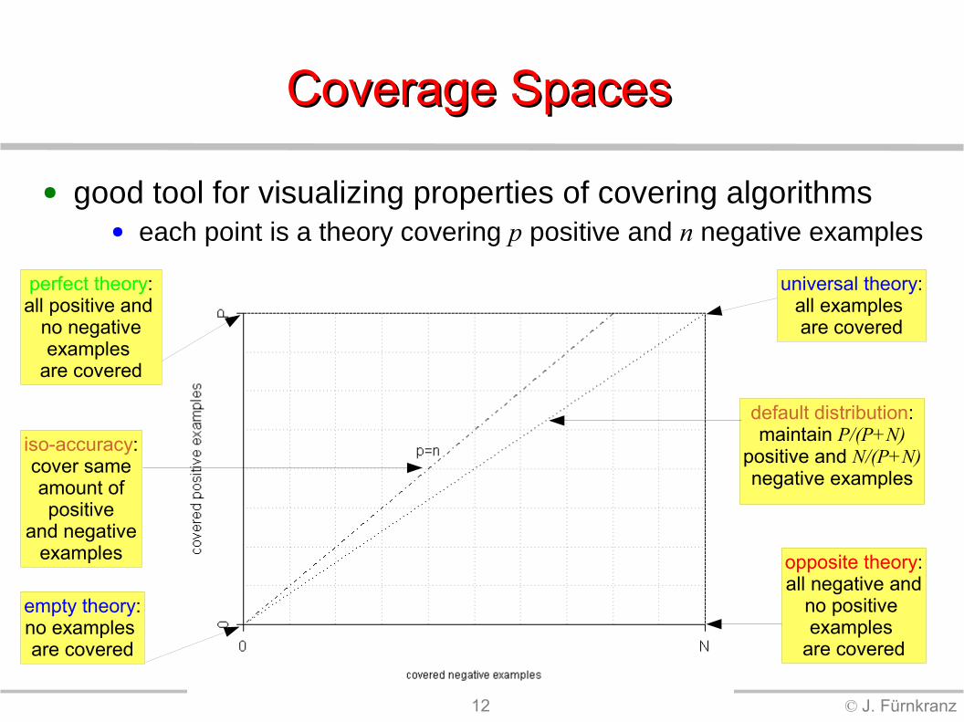
● good tool for visualizing properties of covering algorithms● each point is a theory covering p positive and n negative examples

universal theory:all examples are covered

empty theory:no examples are covered

perfect theory:all positive and

no negativeexamples

are covered

default distribution:maintain P/(P+N)

positive and N/(P+N)negative examples

opposite theory:all negative and

no positive examples

are covered

iso-accuracy:cover sameamount ofpositive

and negativeexamples

13 © J. Fürnkranz

Covering StrategyCovering Strategy

● Covering or Separate-and-Conquer rule learning learning algorithms learn one rule at a time

● This corresponds to a path in coverage space:

● The empty theory R0 (no rules) corresponds to (0,0)

● Adding one rule never decreases p or n because adding a rule covers more examples (generalization)

● The universal theory R+ (all examples are positive) corresponds to (N,P)

+

14 © J. Fürnkranz

Top-Down Hill-ClimbingTop-Down Hill-Climbing

Top-Down Strategy: A rule is successively specialized

1. Start with an empty rule R that covers all examples

2. Evaluate all possible ways to add a condition to R

3. Choose the best one (according to some heuristic)

4. If R is satisfactory, return it

5. Else goto 2.

● Almost all greedy s&c rule learning systems use this strategy

15 © J. Fürnkranz

Top-Down Hill-ClimbingTop-Down Hill-Climbing● successively extends a rule by adding conditions

● This corresponds to a path in coverage space: The rule p:-true covers all

examples (universal theory) Adding a condition never

increases p or n (specialization) The rule p:-false covers

no examples (empty theory)

● which conditions are selected depends on a heuristic function that estimates the quality of the rule

16 © J. Fürnkranz

Rule Learning HeuristicsRule Learning Heuristics

● Adding a rule should increase the number of covered negative examples as little as

possible (do not decrease consistency) increase the number of covered positive examples as much

as possible (increase completeness)● An evaluation heuristic should therefore trade off these two

extremes Example: Laplace heuristic

● grows with ● grows with

Note: Precision is not a good heuristic. Why?

hLap=p1

pn2

hPrec=p

pn

p∞n0

17 © J. Fürnkranz

ExampleExample

p n Laplace p-n2 2 0.5000 0.5000 0

Mild 3 1 0.7500 0.6667 24 2 0.6667 0.6250 22 3 0.4000 0.4286 -14 0 1.0000 0.8333 4

Rain 3 2 0.6000 0.5714 13 4 0.4286 0.4444 -1

Normal 6 1 0.8571 0.7778 53 3 0.5000 0.5000 06 2 0.7500 0.7000 4

Condition PrecisionHot

Temperature =ColdSunny

Outlook = Overcast

Humidity = High

Windy = TrueFalse

● Heuristics Precision and Laplace add the condition Outlook= Overcast to the (empty) rule stop and try to learn the next rule

● Heuristic Accuracy / p − n adds Humidity = Normal continue to refine the rule (until no covered negative)

18 © J. Fürnkranz

Isometrics in Coverage SpaceIsometrics in Coverage Space

● Isometrics are lines that connect points for which a function in p and n has equal values Examples: Isometrics for heuristics h

p = p and h

n = -n

19 © J. Fürnkranz

Precision (Confidence)Precision (Confidence)

● basic idea:percentage of positive examples among covered examples

● effects: rotation around origin

(0,0) all rules with same

angle equivalent in particular, all rules

on P/N axes are equivalent

hPrec=p

pn

20 © J. Fürnkranz

Entropy and Gini Index Entropy and Gini Index

effects: entropy and Gini index are

equivalent like precision, isometrics

rotate around (0,0) isometrics are symmetric

around 45o line a rule that only covers

negative examples is as good as a rule that only covers positives

hEnt=− ppn

log2p

pn n

pnlog2

npn

hGini=1− ppn

2

− npn

2

≃ pn pn2

These will be explainedlater (decision trees)

21 © J. Fürnkranz

Accuracy Accuracy

● basic idea:percentage of correct classifications (covered positives plus uncovered negatives)

● effects: isometrics are parallel

to 45o line covering one positive

example is as good as not covering one negative example

hAcc=pN−n

PN≃ p−n Why are they

equivalent?

22 © J. Fürnkranz

Weighted Relative AccuracyWeighted Relative Accuracy

● Two Basic ideas: Precision Gain: compare precision to precision of a rule that

classifies randomly

Coverage: Multiply with the percentage of covered examples

● Resulting formula:

one can show that sorts rules in exactly the same way as

ppn

−P

PN

pnPN

hWRA=pn

PN

ppn

−P

PN

hWRA '= pP−

nN

23 © J. Fürnkranz

Weighted Relative Accuracy Weighted Relative Accuracy

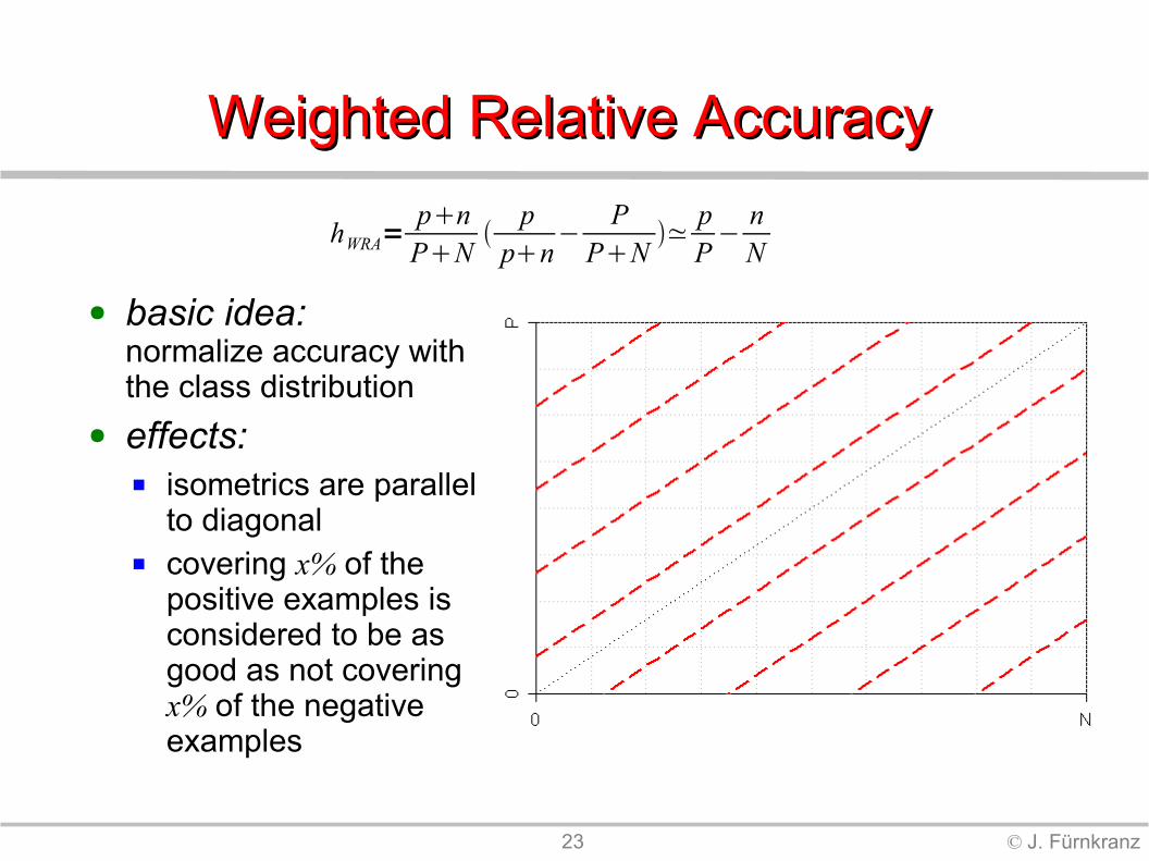
● basic idea:normalize accuracy with the class distribution

● effects: isometrics are parallel

to diagonal covering x% of the

positive examples isconsidered to be as good as not covering x% of the negative examples

hWRA=pnPN

p

pn−

PPN

≃pP−

nN

24 © J. Fürnkranz

Linear Cost MetricLinear Cost Metric

● Accuracy and weighted relative accuracy are only two special cases of the general case with linear costs: costs c mean that covering 1 positive example is as good

as not covering c/(1-c) negative examples

The general form is then● the isometrics of hcost are parallel lines with slope (1-c)/c

hcost=cp−1−cn

c measure

½ accuracy

N/(P+N) weighted relative accuracy

0 excluding negatives at all costs

1 covering positives at all costs

25 © J. Fürnkranz

Relative Cost MetricRelative Cost Metric

● Defined analogously to the Linear Cost Metric● Except that the trade-off is between the normalized

values of p and n between true positive rate p/P and false positive rate n/N

The general form is then● the isometrics of hcost are parallel lines with slope (1-c)/c

● The plots look the same as for the linear cost metric but the semantics of the c value is different:

● for hcost it does not include the example distribution● for hrcost it includes the example distribution

hrcost=c pP−1−c n

N

26 © J. Fürnkranz

Laplace-Estimate Laplace-Estimate

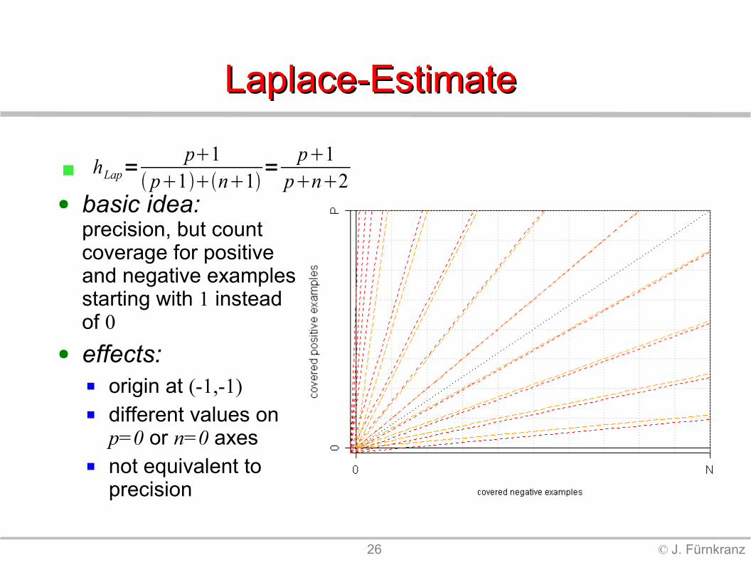
● basic idea:precision, but count coverage for positive and negative examples starting with 1 instead of 0

● effects: origin at (-1,-1) different values on

p=0 or n=0 axes not equivalent to

precision

hLap=p1

p1n1=

p1pn2

27 © J. Fürnkranz

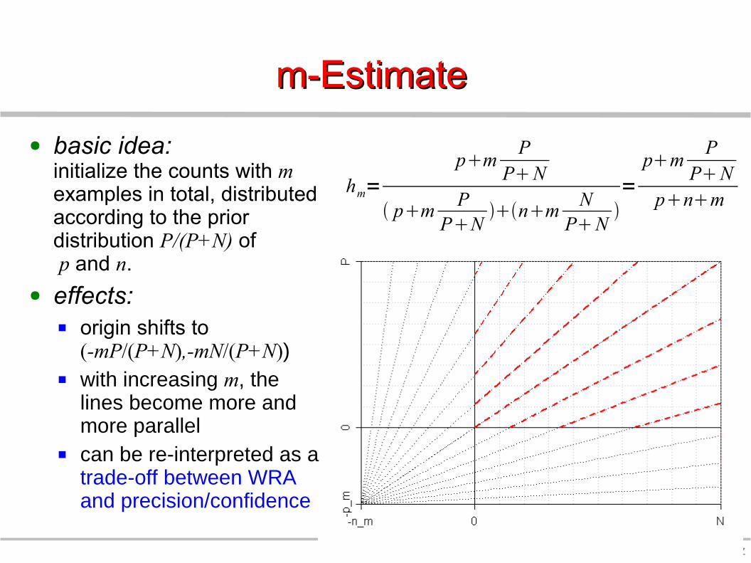
m-Estimate m-Estimate ● basic idea:

initialize the counts with m examples in total, distributed according to the prior distribution P/(P+N) of p and n.

● effects: origin shifts to

(-mP/(P+N),-mN/(P+N)) with increasing m, the

lines become more and more parallel

can be re-interpreted as a trade-off between WRA and precision/confidence

hm=pm P

PN

pm PPN

nm NPN

=

pm PPN

pnm

28 © J. Fürnkranz

Generalized m-EstimateGeneralized m-Estimate

● One can re-interpret the m-Estimate: Re-interpret c = N/(P+N) as a cost factor like in the general

cost metric Re-interpret m as a trade-off between precision and cost-

metric● m = 0: precision (independent of cost factor)● m∞: the isometrics converge towards the parallel isometrics of

the cost metric● Thus, the generalized m-Estimate may be viewed as a

means of trading off between precision and the cost metric

29 © J. Fürnkranz

Optimizing Precision Optimizing Precision ● Precision tries to pick the steepest continuation of the curve

● tries to maximize the area under this curve (→ AUC: Area Under the ROC Curve)

● no particular angle of isometrics is preferred, i.e. no preference for a certain cost model

30 © J. Fürnkranz

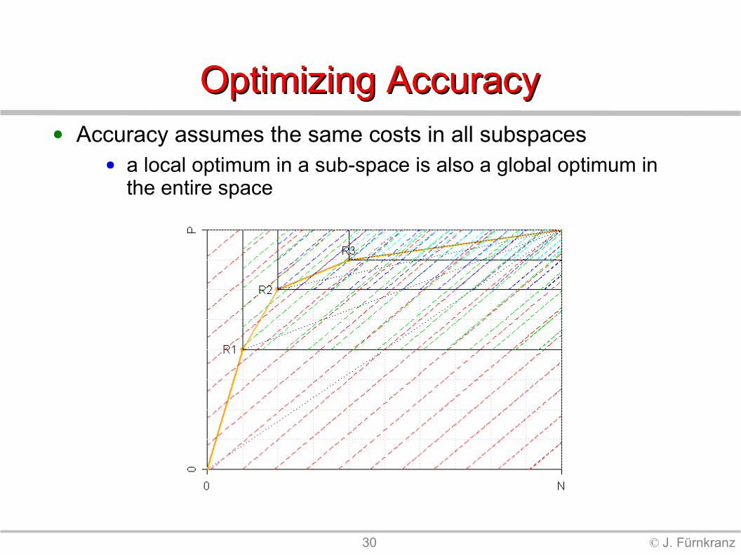
Optimizing AccuracyOptimizing Accuracy● Accuracy assumes the same costs in all subspaces

● a local optimum in a sub-space is also a global optimum in the entire space

31 © J. Fürnkranz

Summary of Rule Learning HeuristicsSummary of Rule Learning Heuristics● There are two basic types of (linear) heuristics.

precision: rotation around the origin cost metrics: parallel lines

● They have different goals precision picks the steepest continuation for the curve for

unkown costs linear cost metrics pick the best point according to known or

assumed costs

● The m-heuristic may be interpreted as a trade-off between the two prototypes parameter c chooses the cost model parameter m chooses the “degree of parallelism”

32 © J. Fürnkranz

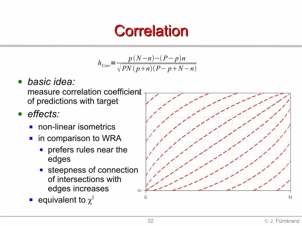
CorrelationCorrelation

● basic idea:measure correlation coefficient of predictions with target

● effects: non-linear isometrics in comparison to WRA

● prefers rules near the edges

● steepness of connection of intersections with edges increases

equivalent to χ2

hCorr=p N−n−P− pn

PN pnP− pN−n

33 © J. Fürnkranz

Foil GainFoil Gain

(c is the precision of the parent rule)

h foil=−plog 2 c−log2p

pn

34 © J. Fürnkranz

Which Heuristic is Best?Which Heuristic is Best?

● There have been many proposals for different heuristics and many different justifications for these proposals some measures perform better on some datasets, others on

other datasets

● Large-Scale Empirical Comparison: 27 training datasets

● on which parameters of the heuristics were tuned) 30 independent datasets

● which were not seen during optimization Goals:

● see which heuristics perform best● determine good parameter values for parametrized functions

35 © J. Fürnkranz

Best Parameter SettingsBest Parameter Settings

for m-estimate: m = 22.5

for relative cost metric: c = 0.342

36 © J. Fürnkranz

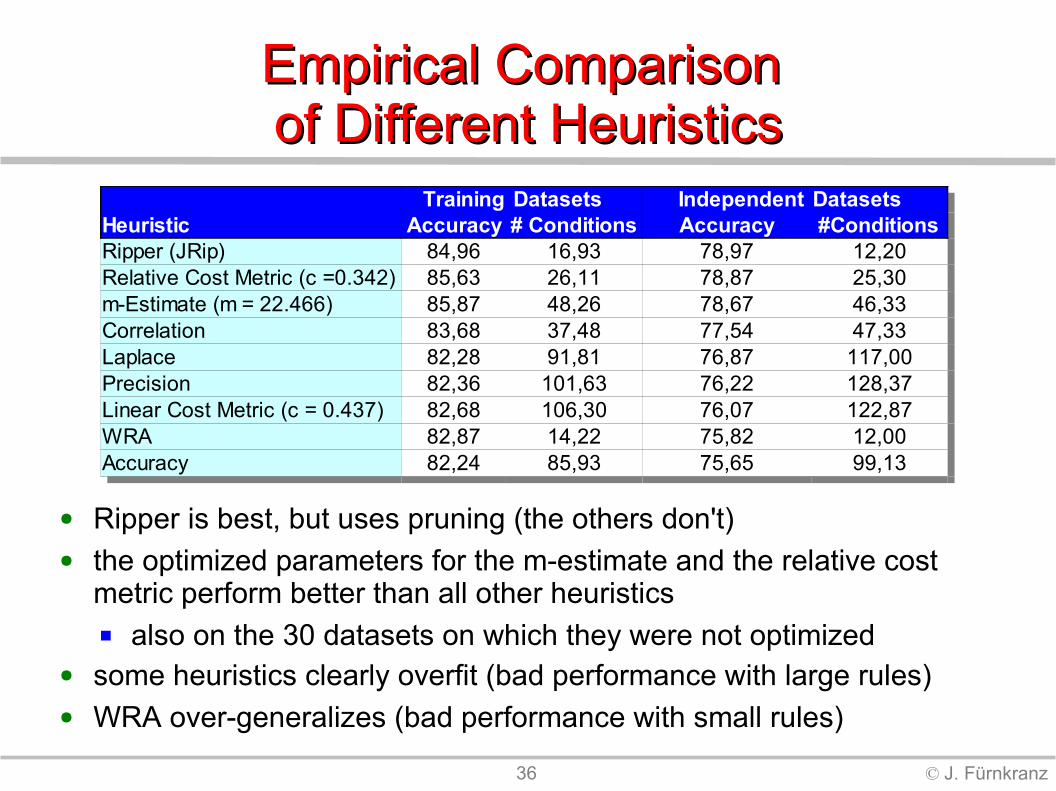
Empirical Comparison Empirical Comparison of Different Heuristicsof Different Heuristics

Training

84,96 16,93 78,97 12,2085,63 26,11 78,87 25,3085,87 48,26 78,67 46,3383,68 37,48 77,54 47,33

Laplace 82,28 91,81 76,87 117,0082,36 101,63 76,22 128,3782,68 106,30 76,07 122,87

WRA 82,87 14,22 75,82 12,0082,24 85,93 75,65 99,13

Datasets Independent DatasetsHeuristic Accuracy # Conditions Accuracy #ConditionsRipper (JRip)Relative Cost Metric (c =0.342)m-Estimate (m = 22.466)Correlation

PrecisionLinear Cost Metric (c = 0.437)

Accuracy

● Ripper is best, but uses pruning (the others don't)● the optimized parameters for the m-estimate and the relative cost

metric perform better than all other heuristics also on the 30 datasets on which they were not optimized

● some heuristics clearly overfit (bad performance with large rules)● WRA over-generalizes (bad performance with small rules)

37 © J. Fürnkranz

Overfitting Overfitting

● Overfitting Given

● a fairly general model class ● enough degrees of freedom

you can always find a model that explains the data● even if the data contains error (noise in the data)● in rule learning: each example is a rule

● Such concepts do not generalize well! → Pruning

38 © J. Fürnkranz

Overfitting - IllustrationOverfitting - Illustration

Prediction for this value of x?

Polynomial degree 1(linear function)

Polynomial degree 4(n-1 degrees can always fit n points)

□ here

□ or here ?

39 © J. Fürnkranz

OverfittingOverfitting

● Eine perfekte Anpassung an die gegebenen Daten ist nicht immer sinnvoll Daten könnten fehlerhaft sein

● z.B. zufälliges Rauschen (Noise) Die Klasse der gewählten Funktionen könnte nicht geeignet sein

● eine perfekte Anpassung an die Trainingsdaten ist oft gar nicht möglich

● Daher ist es oft günstig, die Daten nur ungefähr anzupassen bei Kurven:

● nicht alle Punkte müssen auf der Kurve liegen beim Konzept-Lernen:

● nicht alle positiven Beispiele müssen von der Theorie abgedeckt werden

● einige negativen Beispiele dürfen von der Theorie abgedeckt werden

40 © J. Fürnkranz

OverfittingOverfitting

beim Konzept-Lernen: nicht alle positiven Beispiele müssen von der Theorie

abgedeckt werden einige negativen Beispiele dürfen von der Theorie

abgedeckt werden

41 © J. Fürnkranz

Komplexität von KonzeptenKomplexität von Konzepten

● Je weniger komplex ein Konzept ist, desto geringer ist die Gefahr, daß es sich zu sehr den Daten anpaßt Für ein Polynom n-ten Grades kann man n+1 Parameter

wählen, um die Funktion an alle Punkte anzupassen● Daher wird beim Lernen darauf geachtet, die Größe der

Konzepte klein zu halten eine kurze Regel, die viele positive Beispiele erklärt (aber

eventuell auch einige negative) ist oft besser als eine lange Regel, die nur einige wenige positive Beispiele erklärt.

● Pruning: komplexe Regeln werden zurechtgestutzt Pre-Pruning:

● während des Lernens Post-Pruning:

● nach dem Lernen

42 © J. Fürnkranz

Pre-Pruning Pre-Pruning

● keep a theory simple while it is learned

● decide when to stop adding conditions to a rule (relax consistency constraint)

● decide when to stop adding rules to a theory(relax completeness constraint)

efficient but not accurate

Rule set with three rules á 3, 2, and 2 conditions

Pre-pruning decisions

43 © J. Fürnkranz

Pre-Pruning HeuristicsPre-Pruning Heuristics

1. Thresholding a heuristic value require a certain minimum value of the search heuristic e.g.: Precision > 0.8.

2. Foil's Minimum Description Length Criterion the length of the theory plus the exceptions (misclassified

examples) must be shorter than the length of the examples by themselves

lengths are measured in bits (information content)3. CN2's Significance Test

tests whether the distribution of the examples covered by a rule deviates significantly from the distribution of the examples in the entire training set

if not, discard the rule

44 © J. Fürnkranz

Minimum Coverage FilteringMinimum Coverage Filtering

positive examples (support) all examples (coverage)

filter rules that do not cover a minimum number of

45 © J. Fürnkranz

Support/Confidence FilteringSupport/Confidence Filtering

● filter rules that cover not enough positive

examples (p < suppmin) are not precise enough

(hprec < confmin)● effects:

all but a region around (0,P) is filtered

→ we will return to support/confidence in the context of association rule learning algorithms!

46 © J. Fürnkranz

CN2's likelihood ratio statisticsCN2's likelihood ratio statistics

● basic idea:measure significant deviation from prior probability distribution

● effects: non-linear isometrics

● similar to m-estimate● but prefer rules near the

edges distributed χ2

significance levels 95% (dark) and 99% (light grey)

hLRS=2 p log pe p

n log nen e p= pn P

PN; en= pn N

PN

are the expected number of positive and negative examplein the p+n covered examples.

47 © J. Fürnkranz

CorrelationCorrelation

● basic idea:measure correlation coefficient of predictions with target

● effects: non-linear isometrics in comparison to WRA

● prefers rules near the edges

● steepness of connection of intersections with edges increases

equivalent to χ2

grey area = cutoff of 0.3

hCorr=p N−n−P− pn

PN pnP− pN−n

48 © J. Fürnkranz

MDL-Pruning in FoilMDL-Pruning in Foil

● based on the Minimum Description Length-Principle (MDL) is it more effective to transmit the rule or the covered examples?

● compute the information contents of the rule (in bits)● compute the information contents of the examples (in bits)● if the rule needs more bits than the examples it covers, on can

directly transmit the examples → no need to further refine the rule Details → (Quinlan, 1990)

● doesn't work all that well if rules have expections (i.e., are inconsistent), the negative

examples must be encoded as well● they must be transmitted, otherwise the receiver could not

reconstruct which examples do not conform to the rule finding a minimal encoding (in the information-theoretic sense)

is practically impossible

49 © J. Fürnkranz

Foil's MDL-based Stopping CriterionFoil's MDL-based Stopping Criterion

● basic idea:compare the encoding length of the rule l(r) to the encoding length hMDL of the example. we assume l(r) = c constant

● effects: equivalent to filtering on

support because function only

depends on p

hMDL=log2PN log2 PNp costs for transmitting

which of the P+Nexamples are covered

and positive

costs for transmitting how many examples we have

(can be ignored)

50 © J. Fürnkranz

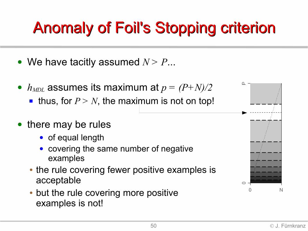
Anomaly of Foil's Stopping criterionAnomaly of Foil's Stopping criterion

● We have tacitly assumed N > P...

● hMDL assumes its maximum at p = (P+N)/2 thus, for P > N, the maximum is not on top!

● there may be rules ● of equal length● covering the same number of negative

examples● the rule covering fewer positive examples is

acceptable● but the rule covering more positive

examples is not!

51 © J. Fürnkranz

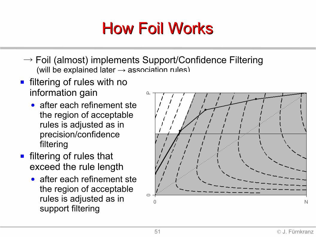
How Foil WorksHow Foil Works

filtering of rules with no information gain● after each refinement step,

the region of acceptable rules is adjusted as in precision/confidence filtering

filtering of rules that exceed the rule length● after each refinement step,

the region of acceptable rules is adjusted as in support filtering

→ Foil (almost) implements Support/Confidence Filtering (will be explained later → association rules)

52 © J. Fürnkranz

Pre-Pruning SystemsPre-Pruning Systems

● Foil: Search heuristic: Foil Gain Pruning: MDL-Based

● CN2: Search heuristic: Laplace/m-heuristic Pruning: Likelihood Ratio

● Fossil: Search heuristic: Correlation Pruning: Threshold

53 © J. Fürnkranz

Post PruningPost Pruning

54 © J. Fürnkranz

Post-Pruning: ExamplePost-Pruning: Example

IF T=hot AND H=high AND O=sunny AND W=false THEN noIF T=hot AND H=high AND O=sunny AND W=true THEN no IF T=hot AND H=high AND O=overcast AND W=false THEN yes IF T=cool AND H=normal AND O=rain AND W=false THEN yes IF T=cool AND H=normal AND O=overcast AND W=true THEN yes IF T=mild AND H=high AND O=sunny AND W=false THEN no IF T=cool AND H=normal AND O=sunny AND W=false THEN yes IF T=mild AND H=normal AND O=rain AND W=false THEN yes IF T=mild AND H=normal AND O=sunny AND W=true THEN yes IF T=mild AND H=high AND O=overcast AND W=true THEN yes IF T=hot AND H=normal AND O=overcast AND W=false THEN yes IF T=mild AND H=high AND O=rain AND W=true THEN no IF T=cool AND H=normal AND O=rain AND W=true THEN no IF T=mild AND H=high AND O=rain AND W=false THEN yes

55 © J. Fürnkranz

Reduced Error Pruning Reduced Error Pruning

● basic idea optimize the accuracy of a rule set on a separate pruning set

0.split training data into a growing and a pruning set

1.learn a complete and consistent rule set covering all positive examples and no negative examples

2.as long as the error on the pruning set does not increase

● delete condition or rule that results in the largest reduction of error on the pruning set

3.return the remaining rules

● accurate but not efficient O(n4)

57 © J. Fürnkranz

Incremental Incremental Reduced Error PruningReduced Error Pruning

● Prune each rule right after it is learned:

1. split training data into a growing and a pruning set

2. learn a consistent rule covering only positive examples

3. delete conditions as long as the error on the pruning set does not increase

4. if the rule is better than the default rule, add it to the rule set and goto 1.

● More accurate, much more efficient because it does not learn overly complex intermediate concept REP: O(n4) I-REP: O(n log2n)

● Subsequently used in the RIPPER (JRip in Weka) rule learner (Cohen, 1995)

59 © J. Fürnkranz

Multi-class problems Multi-class problems

GOAL: discriminate c classes from each other

PROBLEM: many learning algorithms are only suitable for binary (2-class) problems

SOLUTION: "Class binarization": Transform an c-class problem into a series of 2-class problems

60 © J. Fürnkranz

Class Binarization for Rule LearningClass Binarization for Rule Learning

● None class of a rule is defined by the majority of covered

examples decision lists, CN2 (Clark & Niblett 1989)

● One-against-all / unordered foreach class c: label its examples positive, all others

negative CN2 (Clark & Boswell 1991), Ripper -a unordered

● Ordered sort classes - learn first against rest - remove first - repeat Ripper (Cohen 1995)

● Error Correcting Output Codes (Dietterich & Bakiri, 1995) generalized by (Allwein, Schapire, & Singer, JMLR 2000)

61 © J. Fürnkranz

One-against-all binarizationOne-against-all binarization

Treat each class as a separate concept: c binary problems, one for each class label examples of one class positive, all others negative

62 © J. Fürnkranz

PredictionPrediction● It can happen that multiple rules fire for a class

no problem for concept learning (all rules say +) but problematic for multi-class learning

● because each rule may predict a different class Typical solution:

● use rule with the highest precision for prediction more complex approaches are possible: e.g., voting

● It can happen that no rule fires on a class no problem for concept learning (the example is then -) but problematic for multi-class learning

● because it remains unclear which class to select Typical solution: predict the largest class more complex approaches:

● e.g., rule stretching: find the most similar rule to an example

63 © J. Fürnkranz

Round Robin LearningRound Robin Learning(aka (aka Pairwise ClassificationPairwise Classification))

c(c-1)/2 problems each class against each

other class

✔ smaller training sets✔ simpler decision

boundaries✔ larger margins

64 © J. Fürnkranz

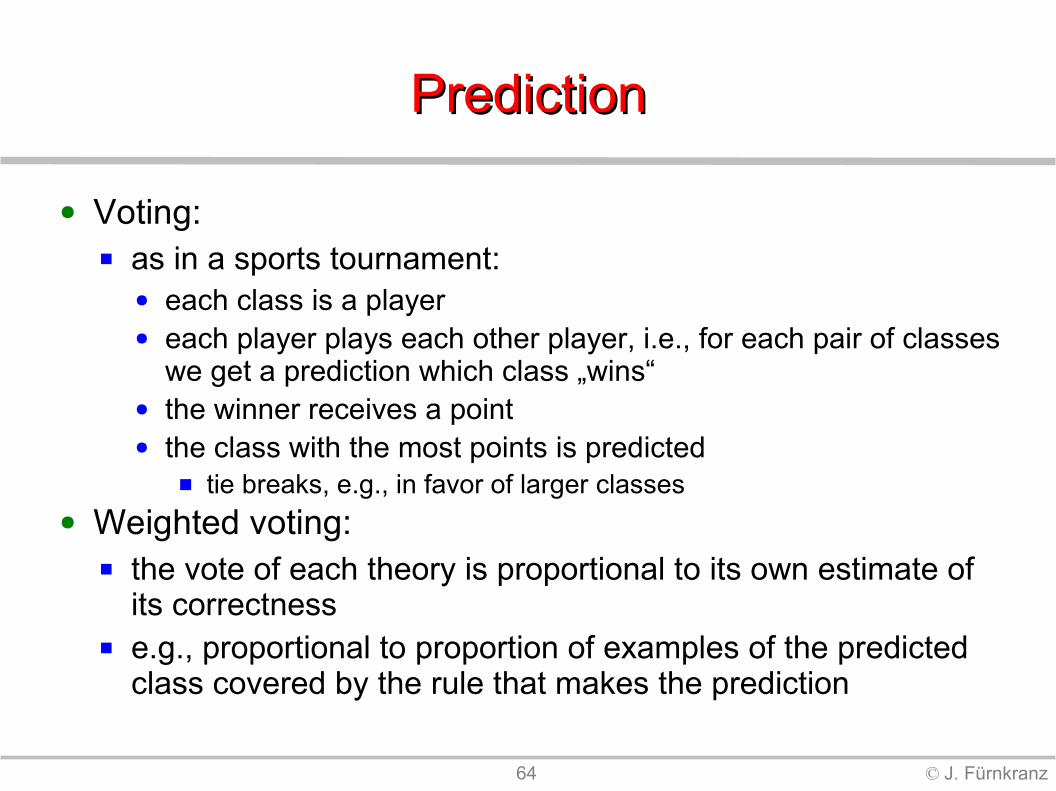
PredictionPrediction

● Voting: as in a sports tournament:

● each class is a player● each player plays each other player, i.e., for each pair of classes

we get a prediction which class „wins“● the winner receives a point● the class with the most points is predicted

tie breaks, e.g., in favor of larger classes● Weighted voting:

the vote of each theory is proportional to its own estimate of its correctness

e.g., proportional to proportion of examples of the predicted class covered by the rule that makes the prediction

65 © J. Fürnkranz

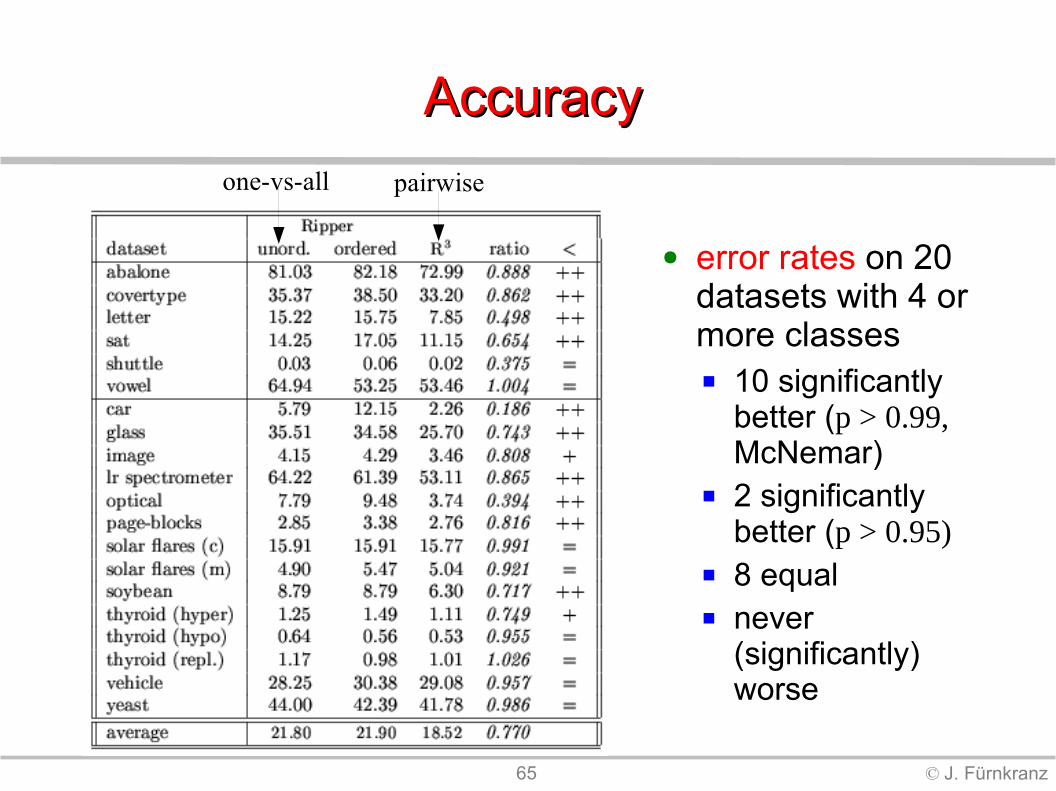
AccuracyAccuracy

● error rates on 20 datasets with 4 or more classes 10 significantly

better (p > 0.99, McNemar)

2 significantly better (p > 0.95)

8 equal never

(significantly) worse

pairwiseone-vs-all

66 © J. Fürnkranz

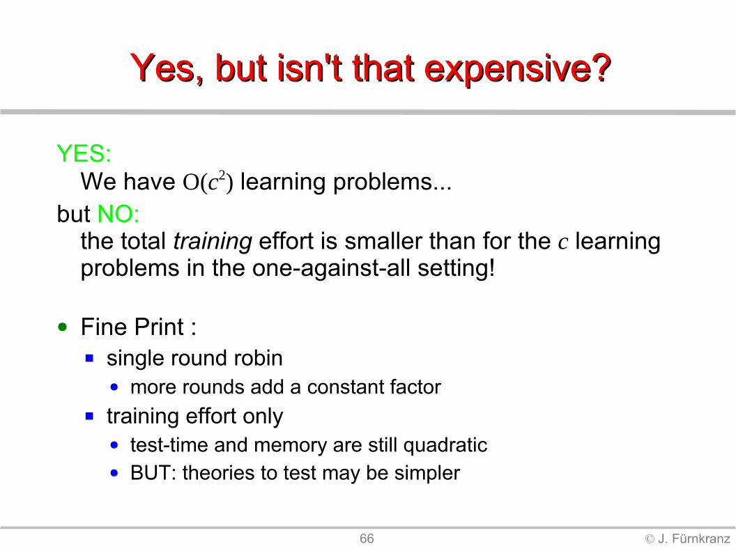
Yes, but isn't that expensive?Yes, but isn't that expensive?

YES: We have O(c2) learning problems...

but NO:the total training effort is smaller than for the c learning problems in the one-against-all setting!

● Fine Print : single round robin

● more rounds add a constant factor training effort only

● test-time and memory are still quadratic● BUT: theories to test may be simpler

67 © J. Fürnkranz

Advantages of Round RobinAdvantages of Round Robin● Accuracy

never lost against one-against-all

often significantly more accurate

● Efficiency proven to be faster than,

e.g., one-against-all, ECOC, boosting...

higher gains for slower base algorithms

● Understandability simpler boundaries/concepts similar to pairwise ranking as

recommended by Pyle (1999)● Example Size Reduction

each binary task is considerably smaller than original data

subtasks might fit into memory where entire task does not

● Easily parallelizable each task is independent of

all other tasks

68 © J. Fürnkranz

A Pathology forA Pathology forTop-Down LearningTop-Down Learning

● Parity problems (e.g. XOR) r relevant binary attributes s irrelevant binary attributes each of the n = r + s attributes has values 0/1 with probability ½ an example is positive if the number of 1's in the relevant

attributes is even, negative otherwise Problem for top-down learning:

● by construction, each condition of the form ai = 0 or a

i = 1

covers approximately 50% positive and 50% negative examples

● irrespective of whether ai is a relevant or an irrelevant attribute

➔ top-down hill-climbing cannot learn this type of concept Typical recommendation:

● use bottom-up learning for such problems

69 © J. Fürnkranz

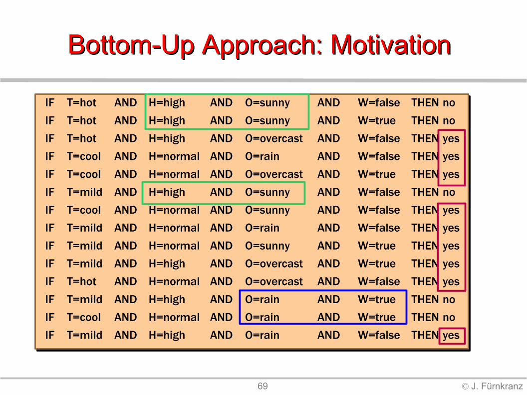
Bottom-Up Approach: Motivation Bottom-Up Approach: Motivation

IF T=hot AND H=high AND O=sunny AND W=false THEN noIF T=hot AND H=high AND O=sunny AND W=true THEN no IF T=hot AND H=high AND O=overcast AND W=false THEN yes IF T=cool AND H=normal AND O=rain AND W=false THEN yes IF T=cool AND H=normal AND O=overcast AND W=true THEN yes IF T=mild AND H=high AND O=sunny AND W=false THEN no IF T=cool AND H=normal AND O=sunny AND W=false THEN yes IF T=mild AND H=normal AND O=rain AND W=false THEN yes IF T=mild AND H=normal AND O=sunny AND W=true THEN yes IF T=mild AND H=high AND O=overcast AND W=true THEN yes IF T=hot AND H=normal AND O=overcast AND W=false THEN yes IF T=mild AND H=high AND O=rain AND W=true THEN no IF T=cool AND H=normal AND O=rain AND W=true THEN no IF T=mild AND H=high AND O=rain AND W=false THEN yes

70 © J. Fürnkranz

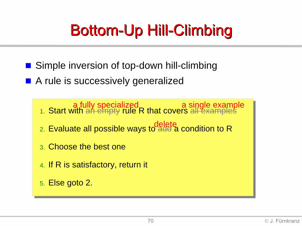
Bottom-Up Hill-ClimbingBottom-Up Hill-Climbing

Simple inversion of top-down hill-climbing

A rule is successively generalized

1. Start with an empty rule R that covers all examples

2. Evaluate all possible ways to add a condition to R

3. Choose the best one

4. If R is satisfactory, return it

5. Else goto 2.

a fully specialized a single example

delete

71 © J. Fürnkranz

A Pathology of Bottom-Up A Pathology of Bottom-Up Hill-ClimbingHill-Climbing

att1 att2 att3

+ 1 1 1

+ 1 0 0

− 0 1 0

− 0 0 1

Target concept att1 = 1 not (reliably) learnable with bottom-up hill-climbing● because no generalization of any seed example will increase

coverage● Hence you either stop or make an arbitrary choice (e.g.,

delete attribute 1)

72 © J. Fürnkranz

Bottom-Up Rule Learning AlgorithmsBottom-Up Rule Learning Algorithms

● AQ-type: select a seed example and search the space of its

generalizations BUT: search this space top-down Examples: AQ (Michalski 1969), Progol (Muggleton 1995)

● based on least general generalizations (lggs) greedy bottom-up hill-climbing BUT: expensive generalization operator

(lgg/rlgg of pairs of seed examples) Examples: Golem (Muggleton & Feng 1990), DLG (Webb 1992), RISE

(Domingos 1995)● Incremental Pruning of Rules:

greedy bottom-up hill-climbing via deleting conditions BUT: start at point previously reached via top-down specialization Examples: I-REP (Fürnkranz & Widmer 1994), Ripper (Cohen 1995)

● language bias: which type of

conditions are allowed (static)

which combinations of condictions are allowed (dynamic)

● search bias: search heuristics search algorithm

(greedy, stochastic, exhaustive)

search strategy (top-down, bottom-up)

● overfitting avoidance bias: pre-pruning

(stopping criteria) post-pruning

74 © J. Fürnkranz

Rules vs. Trees Rules vs. Trees

● Each decision tree can be converted into a rule set→ Rule sets are at least as expressive as decision trees

a decision tree can be viewed as a set of non-overlapping rules

typically learned via divide-and-conquer algorithms (recursive partitioning)

● Many concepts have a shorter description as a rule set exceptions: if one or more attributes are relevant for the

classification of all examples (e.g., parity)● Learning strategies:

Separate-and-Conquer vs. Divide-and-Conquer