learning spark
TRANSCRIPT
2
Learning Spark
Holden Karau
Andy Konwinski
Patrick Wendell
Matei Zaharia
Beijing • Cambridge • Farnham • Köln • Sebastopol • Tokyo

3
Table of Contents
Preface................................................................................................................................................ 5
Audience................................................................................................................................................5
How This Book is Organized..............................................................................................................6
Supporting Books.................................................................................................................................6
Code Examples..................................................................................................................................... 7
Early Release Status and Feedback................................................................................................... 7
Chapter 1. Introduction to Data Analysis with Spark......................................................8
What is Apache Spark?....................................................................................................................... 8
A Unified Stack.....................................................................................................................................8
Who Uses Spark, and For What?......................................................................................................11
A Brief History of Spark.................................................................................................................... 13
Spark Versions and Releases............................................................................................................13
Spark and Hadoop............................................................................................................................. 14
Chapter 2. Downloading and Getting Started...................................................................15
Downloading Spark............................................................................................................................15
Introduction to Spark’s Python and Scala Shells.......................................................................... 16
Introduction to Core Spark Concepts.............................................................................................20
Standalone Applications...................................................................................................................23
Conclusion.......................................................................................................................................... 25
Chapter 3. Programming with RDDs...................................................................................26
RDD Basics.........................................................................................................................................26
Creating RDDs................................................................................................................................... 28
RDD Operations................................................................................................................................ 28
Passing Functions to Spark..............................................................................................................32
Common Transformations and Actions.........................................................................................36
Persistence (Caching)........................................................................................................................46
Conclusion..........................................................................................................................................48
Chapter 4. Working with Key-Value Pairs.........................................................................49
4
Motivation.......................................................................................................................................... 49
Creating Pair RDDs...........................................................................................................................49
Transformations on Pair RDDs.......................................................................................................50
Actions Available on Pair RDDs......................................................................................................60
Data Partitioning................................................................................................................................61
Conclusion.......................................................................................................................................... 70
Chapter 5. Loading and Saving Your Data..........................................................................71
Motivation........................................................................................................................................... 71
Choosing a Format............................................................................................................................. 71
Formats............................................................................................................................................... 72
File Systems........................................................................................................................................88
Compression.......................................................................................................................................89
Databases............................................................................................................................................ 91
Conclusion..........................................................................................................................................93
About the Authors........................................................................................................................95

5
Preface
As parallel data analysis has become increasingly common, practitioners in many fields have
sought easier tools for this task. Apache Spark has quickly emerged as one of the most popular
tools for this purpose, extending and generalizing MapReduce. Spark offers three main benefits.
First, it is easy to use—you can develop applications on your laptop, using a high-level API that
lets you focus on the content of your computation. Second, Spark is fast, enabling interactive use
and complex algorithms. And third, Spark is a general engine, allowing you to combine multiple
types of computations (e.g., SQL queries, text processing and machine learning) that might
previously have required learning different engines. These features make Spark an excellent
starting point to learn about big data in general.
This introductory book is meant to get you up and running with Spark quickly. You’ll learn how
to learn how to download and run Spark on your laptop and use it interactively to learn the API.
Once there, we’ll cover the details of available operations and distributed execution. Finally,
you’ll get a tour of the higher-level libraries built into Spark, including libraries for machine
learning, stream processing, graph analytics and SQL. We hope that this book gives you the
tools to quickly tackle data analysis problems, whether you do so on one machine or hundreds.
Audience
This book targets Data Scientists and Engineers. We chose these two groups because they have
the most to gain from using Spark to expand the scope of problems they can solve. Spark’s rich
collection of data focused libraries (like MLlib) make it easy for data scientists to go beyond
problems that fit on single machine while making use of their statistical background. Engineers,
meanwhile, will learn how to write general-purpose distributed programs in Spark and operate
production applications. Engineers and data scientists will both learn different details from this
book, but will both be able to apply Spark to solve large distributed problems in their respective
fields.
Data scientists focus on answering questions or building models from data. They often have a
statistical or math background and some familiarity with tools like Python, R and SQL. We have
made sure to include Python, and wherever possible SQL, examples for all our material, as well
as an overview of the machine learning and advanced analytics libraries in Spark. If you are a
data scientist, we hope that after reading this book you will be able to use the same
mathematical approaches to solving problems, except much faster and on a much larger scale.
6
The second group this book targets is software engineers who have some experience with Java,
Python or another programming language. If you are an engineer, we hope that this book will
show you how to set up a Spark cluster, use the Spark shell, and write Spark applications to
solve parallel processing problems. If you are familiar with Hadoop, you have a bit of a head
start on figuring out how to interact with HDFS and how to manage a cluster, but either way, we
will cover basic distributed execution concepts.
Regardless of whether you are a data analyst or engineer, to get the most of this book you should
have some familiarity with one of Python, Java, Scala, or a similar language. We assume that
you already have a solution for storing your data and we cover how to load and save data from
many common ones, but not how to set them up. If you don’t have experience with one of those
languages, don’t worry, there are excellent resources available to learn these. We call out some
of the books available in Supporting Books.
How This Book is Organized
The chapters of this book are laid out in such a way that you should be able to go through the
material front to back. At the start of each chapter, we will mention which sections of the
chapter we think are most relevant to data scientists and which sections we think are most
relevant for engineers. That said, we hope that all the material is accessible to readers of either
background.
The first two chapters will get you started with getting a basic Spark installation on your laptop
and give you an idea of what you can accomplish with Apache Spark. Once we’ve got the
motivation and setup out of the way, we will dive into the Spark Shell, a very useful tool for
development and prototyping. Subsequent chapters then cover the Spark programming
interface in detail, how applications execute on a cluster, and higher-level libraries available on
Spark such as Spark SQL and MLlib.
Supporting Books
If you are a data scientist and don’t have much experience with Python, the Learning Python
book is an excellent introduction.
If you are an engineer and after reading this book you would like to expand your data analysis
skills, Machine Learning for Hackers and Doing Data Science are excellent books from O’Reilly.
This book is intended to be accessible to beginners. We do intend to release a deep dive
follow-up for those looking to gain a more thorough understanding of Spark’s internals.
7
Code Examples
All of the code examples found in this book are on GitHub. You can examine them and check
them out from https://github.com/databricks/learning-spark. Code examples are provided in
Java, Scala, and Python.
Tip
Our Java examples are written to work with Java version 6 and higher. Java 8 introduces a new
syntax called “lambdas” that makes writing inline functions much easier, which can simplify
Spark code. We have chosen not to take advantage of this syntax in most of our examples, as
most organizations are not yet using Java 8. If you would like to try Java 8 syntax, you can see
the Databricks blog post on this topic.
Early Release Status and Feedback
This is an early release copy of Learning Spark, and as such we are still working on the text,
adding code examples, and writing some of the later chapters. Although we hope that the book is
useful in its current form, we would greatly appreciate your feedback so we can improve it and
make the best possible finished product. The authors and editors can be reached at
The authors would like to thank the reviewers who offered feedback so far: Juliet Hougland,
Andrew Gal, Michael Gregson, Stephan Jou, Josh Mahonin, and Mike Patterson.
8
Chapter 1. Introduction to Data Analysis with Spark
This chapter provides a high level overview of what Apache Spark is. If you are already familiar
with Apache Spark and its components, feel free to jump ahead to Chapter 2.
What is Apache Spark?
Apache Spark is a cluster computing platform designed to be fast and general-purpose.
On the speed side, Spark extends the popular MapReduce model to efficiently support more
types of computations, including interactive queries and stream processing. Speed is important
in processing large datasets as it means the difference between exploring data interactively and
waiting minutes between queries, or waiting hours to run your program versus minutes. One of
the main features Spark offers for speed is the ability to run computations in memory, but the
system is also faster than MapReduce for complex applications running on disk.
On the generality side, Spark is designed to cover a wide range of workloads that previously
required separate distributed systems, including batch applications, iterative algorithms,
interactive queries and streaming. By supporting these workloads in the same engine, Spark
makes it easy and inexpensive to combine different processing types, which is often necessary in
production data analysis pipelines. In addition, it reduces the management burden of
maintaining separate tools.
Spark is designed to be highly accessible, offering simple APIs in Python, Java, Scala and SQL,
and rich built-in libraries. It also integrates closely with other big data tools. In particular, Spark
can run in Hadoop clusters and access any Hadoop data source.
A Unified Stack
The Spark project contains multiple closely-integrated components. At its core, Spark is a
“computational engine” that is responsible for scheduling, distributing, and monitoring
applications consisting of many computational tasks across many worker machines, or a
computing cluster. Because the core engine of Spark is both fast and general-purpose, it powers
multiple higher-level components specialized for various workloads, such as SQL or machine
learning. These components are designed to interoperate closely, letting you combine them like
libraries in a software project.

9
A philosophy of tight integration has several benefits. First, all libraries and higher level
components in the stack benefit from improvements at the lower layers. For example, when
Spark’s core engine adds an optimization, SQL and machine learning libraries automatically
speed up as well. Second, the costs associated with running the stack are minimized, because
instead of running 5-10 independent software systems, an organization only needs to run one.
These costs include deployment, maintenance, testing, support, and more. This also means that
each time a new component is added to the Spark stack, every organization that uses Spark will
immediately be able to try this new component. This changes the cost of trying out a new type of
data analysis from downloading, deploying, and learning a new software project to upgrading
Spark.
Finally, one of the largest advantages of tight integration is the ability to build applications that
seamlessly combine different processing models. For example, in Spark you can write one
application that uses machine learning to classify data in real time as it is ingested from
streaming sources. Simultaneously analysts can query the resulting data, also in real-time, via
SQL, e.g. to join the data with unstructured log files. In addition, more sophisticated data
engineers can access the same data via the Python shell for ad-hoc analysis. Others might access
the data in standalone batch applications. All the while, the IT team only has to maintain one
software stack.
Figure 1-1. The Spark Stack
Here we will briefly introduce each of the components shown in Figure 1-1.
10
Spark Core
Spark Core contains the basic functionality of Spark, including components for task scheduling,
memory management, fault recovery, interacting with storage systems, and more. Spark Core is
also home to the API that defines Resilient Distributed Datasets (RDDs), which are Spark’s main
programming abstraction. RDDs represent a collection of items distributed across many
compute nodes that can be manipulated in parallel. Spark Core provides many APIs for building
and manipulating these collections.
Spark SQL
Spark SQL provides support for interacting with Spark via SQL as well as the Apache Hive
variant of SQL, called the Hive Query Language (HiveQL). Spark SQL represents database tables
as Spark RDDs and translates SQL queries into Spark operations. Beyond providing the SQL
interface to Spark, Spark SQL allows developers to intermix SQL queries with the programmatic
data manipulations supported by RDDs in Python, Java and Scala, all within a single application.
This tight integration with the the rich and sophisticated computing environment provided by
the rest of the Spark stack makes Spark SQL unlike any other open source data warehouse tool.
Spark SQL was added to Spark in version 1.0.
Shark is a project out of UC Berkeley that pre-dates Spark SQL and is being ported to work on
top of Spark SQL. Shark provides additional functionality so that Spark can act as drop-in
replacement for Apache Hive. This includes a HiveQL shell, as well as a JDBC server that makes
it easy to connect external graphing and data exploration tools.
Spark Streaming
Spark Streaming is a Spark component that enables processing live streams of data. Examples of
data streams include log files generated by production web servers, or queues of messages
containing status updates posted by users of a web service. Spark Streaming provides an API for
manipulating data streams that closely matches the Spark Core’s RDD API, making it easy for
programmers to learn the project and move between applications that manipulate data stored in
memory, on disk, or arriving in real-time. Underneath its API, Spark Streaming was designed to
provide the same degree of fault tolerance, throughput, and scalability that the Spark Core
provides.
MLlib
Spark comes with a library containing common machine learning (ML) functionality called
MLlib. MLlib provides multiple types of machine learning algorithms, including binary
classification, regression, clustering and collaborative filtering, as well as supporting
11
functionality such as model evaluation and data import. It also provides some lower level ML
primitives including a generic gradient descent optimization algorithm. All of these methods are
designed to scale out across a cluster.
GraphX
GraphX is a library added in Spark 0.9 that provides an API for manipulating graphs (e.g., a
social network’s friend graph) and performing graph-parallel computations. Like Spark
Streaming and Spark SQL, GraphX extends the Spark RDD API, allowing us to create a directed
graph with arbitrary properties attached to each vertex and edge. GraphX also provides set of
operators for manipulating graphs (e.g., subgraph and mapVertices) and a library of common
graph algorithms (e.g., PageRank and triangle counting).
Cluster Managers
Under the hood, Spark is designed to efficiently scale up from one to many thousands of
compute nodes. To achieve this while maximizing flexibility, Spark can run over a variety of
cluster managers, including including Hadoop YARN, Apache Mesos, and a simple cluster
manager included in Spark itself called the Standalone Scheduler. If you are just installing Spark
on an empty set of machines, the Standalone Scheduler provides an easy way to get started;
while if you already have a Hadoop YARN or Mesos cluster, Spark’s support for these allows
your applications to also run on them.
Who Uses Spark, and For What?
Because Spark is a general purpose framework for cluster computing, it is used for a diverse
range of applications. In the Preface we outlined two personas that this book targets as readers:
Data Scientists and Engineers. Let’s take a closer look at each of these personas and how they
use Spark. Unsurprisingly, the typical use cases differ across the two personas, but we can
roughly classify them into two categories, data science and data applications.
Of course, these are imprecise personas and usage patterns, and many folks have skills from
both, sometimes playing the role of the investigating Data Scientist, and then “changing hats”
and writing a hardened data processing system. Nonetheless, it can be illuminating to consider
the two personas and their respective use cases separately.
Data Science Tasks
Data Science is the name of a discipline that has been emerging over the past few years centered
around analyzing data. While there is no standard definition, for our purposes a Data Scientist
12
is somebody whose main task is to analyze and model data. Data scientists may have experience
using SQL, statistics, predictive modeling (machine learning), and some programming, usually
in Python, Matlab or R. Data scientists also have experience with techniques necessary to
transform data into formats that can be analyzed for insights (sometimes referred to as data
wrangling).
Data Scientists use their skills to analyze data with the goal of answering a question or
discovering insights. Oftentimes, their workflow involves ad-hoc analysis, and so they use
interactive shells (vs. building complex applications) that let them see results of queries and
snippets of code in the least amount of time. Spark’s speed and simple APIs shine for this
purpose, and its built-in libraries mean that many algorithms are available out of the box.
Sometimes, after the initial exploration phase, the work of a Data Scientist will be
“productionized”, or extended, hardened (i.e. made fault tolerant), and tuned to become a
production data processing application, which itself is a component of a business application.
For example, the initial investigation of a Data Scientist might lead to the creation of a
production recommender system that is integrated into on a web application and used to
generate customized product suggestions to users. Often it is a different person or team that
leads the process of productizing the work of the Data Scientists, and that person is often an
Engineer.
Data Processing Applications
The other main use case of Spark can be described in the context of the Engineer persona. For
our purposes here, we think of Engineers as large class of software developers who use Spark to
build production data processing applications. These developers usually have an understanding
of the principles of software engineering, such as encapsulation, interface design, and Object
Oriented Programming. They frequently have a degree in Computer Science. They use their
engineering skills to design and build software systems that implement a business use case.
For Engineers, Spark provides a simple way to parallelize these applications across clusters, and
hides the complexity of distributed systems programming, network communication and fault
tolerance. The system gives enough control to monitor, inspect and tune applications while
allowing common tasks to be implemented quickly. The modular nature of the API (based on
passing distributed collections of objects) makes it easy to factor work into reusable libraries
and test it locally.
Spark’s users choose to use it for their data processing applications because it provides a wide
variety of functionality, is easy to learn and use, and is mature and reliable.
13
A Brief History of Spark
Spark is an open source project that has been built and is maintained by a thriving and diverse
community of developers from many different organizations. If you or your organization are
trying Spark for the first time, you might be interested in the history of the project. Spark started
in 2009 as a research project in the UC Berkeley RAD Lab, later to become the AMPLab. The
researchers in the lab had previously been working on Hadoop MapReduce, and observed that
MapReduce was inefficient for iterative and interactive computing jobs. Thus, from the
beginning, Spark was designed to be fast for interactive queries and iterative algorithms,
bringing in ideas like support for in-memory storage and efficient fault recovery.
Research papers were published about Spark at academic conferences and soon after its creation
in 2009, it was already 10—20x faster than MapReduce for certain jobs.
Some of Spark’s first users were other groups inside of UC Berkeley, including machine learning
researchers such as the the Mobile Millennium project, which used Spark to monitor and predict
traffic congestion in the San Francisco bay Area. In a very short time, however, many external
organizations began using Spark, and today, over 50 organizations list themselves on the Spark
PoweredBy page [1], and dozens speak about their use cases at Spark community events such as
Spark Meetups [2] and the Spark Summit [3]. Apart from UC Berkeley, major contributors to the
project currently include Yahoo!, Intel and Databricks.
In 2011, the AMPLab started to develop higher-level components on Spark, such as Shark (Hive
on Spark) and Spark Streaming. These and other components are often referred to as the
Berkeley Data Analytics Stack (BDAS) [4]. BDAS includes both components of Spark and other
software projects that complement it, such as the Tachyon memory manager.
Spark was first open sourced in March 2010, and was transferred to the Apache Software
Foundation in June 2013, where it is now a top-level project.
Spark Versions and Releases
Since its creation Spark has been a very active project and community, with the number of
contributors growing with each release. Spark 1.0 had over 100 individual contributors. Though
the level of activity has rapidly grown, the community continues to release updated versions of
Spark on a regular schedule. Spark 1.0 was released in May 2014. This book focuses primarily on
Spark 1.0 and beyond, though most of the concepts and examples also work in earlier versions.

14
Spark and Hadoop
Spark can create distributed datasets from any file stored in the Hadoop distributed file system
(HDFS) or other storage systems supported by Hadoop (including your local file system,
Amazon S3, Cassandra, Hive, HBase, etc). Spark supports text files, SequenceFiles, Avro,
Parquet, and any other Hadoop InputFormat. We will look at interacting with these data sources
in the loading and saving chapter.
[1]https://cwiki.apache.org/confluence/display/SPARK/Powered+By+Spark
[2]http://www.meetup.com/spark-users/
[3]http://spark-summit.org
[4]https://amplab.cs.berkeley.edu/software
15
Chapter 2. Downloading and Getting Started
In this chapter we will walk through the process of downloading and running Spark in local
mode on a single computer. This chapter was written for anybody that is new to Spark, including
both Data Scientists and Engineers.
Spark can be used from Python, Java or Scala. To benefit from this book, you don’t need to be an
expert programmer, but we do assume that you are comfortable with the basic syntax of at least
one of these languages. We will include examples in all languages wherever possible.
Spark itself is written in Scala, and runs on the Java Virtual Machine (JVM). To run Spark on
either your laptop or a cluster, all you need is an installation of Java 6 (or newer). If you wish to
use the Python API you will also need a Python interpreter (version 2.6 or newer) . Spark does
not yet work with Python 3.
Downloading Spark
The first step to using Spark is to download and unpack it into a usable form. Let’s start by
downloading a recent precompiled released version of Spark. Visit
http://spark.apache.org/downloads.html, then under “Pre-built packages”, next to “For Hadoop
1 (HDP1, CDH3)”, click “direct file download”. This will download a compressed tar file, or
“tarball,” called spark-1.0.0-bin-hadoop1.tgz.
If you want to use Spark with another Hadoop version, those are also available from
http://spark.apache.org/downloads.html but will have slightly different file names. Building
from source is also possible, and you can find the latest source code on GitHub at
http://github.com/apache/spark.
Note
Most Unix and Linux variants, including Mac OS X, come with a command-line tool called tar
that can be used to unpack tar files. If your operating system does not have the tar command
installed, try searching the Internet for a free tar extractor—for example, on Windows, you may
wish to try 7-Zip.
Now that we have downloaded Spark, let’s unpack it and take a look at what comes with the
default Spark distribution. To do that, open a terminal, change to the directory where you
downloaded Spark, and untar the file. This will create a new directory with the same name but

16
without the final .tgz suffix. Change into the directory, and see what’s inside. You can use the
following commands to accomplish all of that.
cd ~
tar -xf spark-1.0.0-bin-hadoop1.tgz
cd spark-1.0.0-bin-hadoop1
ls
In the line containing the tar command above, the x flag tells tar we are extracting files, and the f
flag specifies the name of the tarball. The ls command lists the contents of the Spark directory.
Let’s briefly consider the names and purpose of some of the more important files and directories
you see here that come with Spark.
README.md - Contains short instructions for getting started with Spark.
bin - Contains executable files that can be used to interact with Spark in various ways, e.g. the
spark-shell, which we will cover later in this chapter, is in here.
core, streaming, python - source code of major components of the Spark project.
examples - contains some helpful Spark standalone jobs that you can look at and run to learn about
the Spark API.
Don’t worry about the large number of directories and files the Spark project comes with; we
will cover most of these in the rest of this book. For now, let’s dive in right away and try out
Spark’s Python and Scala shells. We will start by running some of the examples that come with
Spark. Then we will write, compile and run a simple Spark Job of our own.
All of the work we will do in this chapter will be with Spark running in “local mode”, i.e.
non-distributed mode, which only uses a single machine. Spark can run in a variety of different
modes, or environments. Beyond local mode, Spark can also be run on Mesos, YARN, on top of a
Standalone Scheduler that is included in the Spark distribution. We will cover the various
deployment modes in detail in chapter (to come).
Introduction to Spark’s Python and Scala Shells
Spark comes with interactive shells that make ad-hoc data analysis easy. Spark’s shells will feel
familiar if you have used other shells such as those in R, Python, and Scala, or operating system
shells like Bash or the Windows command prompt.
Unlike most other shells, however, which let you manipulate data using the disk and memory on
a single machine, Spark’s shells allow you to interact with data that is distributed on disk or in

17
memory across many machines, and Spark takes care of automatically distributing this
processing.
Because Spark can load data into memory, many distributed computations, even ones that
process terabytes of data across dozens of machines, can finish running in a few seconds. This
makes the sort of iterative, ad-hoc, and exploratory analysis commonly done in shells a good fit
for Spark. Spark provides both Python and Scala shells that have been augmented to support
connecting to a cluster.
Note
Most of this book includes code in all of Spark’s languages, but interactive shells are only
available in Python and Scala. Because a shell is very useful for learning the API, we recommend
using one of these languages for these examples even if you are a Java developer. The API is the
same in every language.
The easiest way to demonstrate the power of Spark’s shells is to start using one of them for some
simple data analysis. Let’s walk through the example from the Quick Start Guide in the official
Spark documentation [5].
The first step is to open up one of Spark’s shells. To open the Python version of the Spark Shell,
which we also refer to as the PySpark Shell, go into your Spark directory and type:
bin/pyspark
(Or bin\pyspark in Windows.) To open the Scala version of the shell, type:
bin/spark-shell
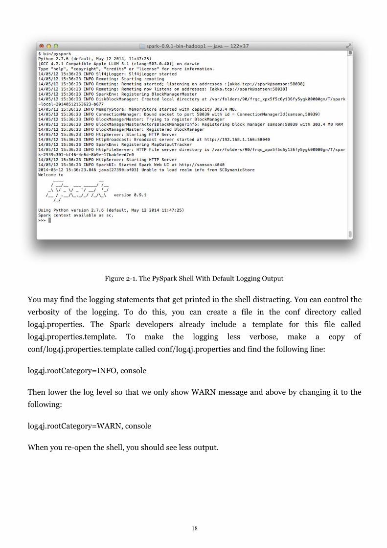
The shell prompt should appear within a few seconds. When the shell starts, you will notice a lot
of log messages. You may need to hit [Enter] once to clear the log output, and get to a shell
prompt. Figure Figure 2-1 shows what the PySpark shell looks like when you open it.
18
Figure 2-1. The PySpark Shell With Default Logging Output
You may find the logging statements that get printed in the shell distracting. You can control the
verbosity of the logging. To do this, you can create a file in the conf directory called
log4j.properties. The Spark developers already include a template for this file called
log4j.properties.template. To make the logging less verbose, make a copy of
conf/log4j.properties.template called conf/log4j.properties and find the following line:
log4j.rootCategory=INFO, console
Then lower the log level so that we only show WARN message and above by changing it to the
following:
log4j.rootCategory=WARN, console
When you re-open the shell, you should see less output.

19
Figure 2-2. The PySpark Shell With Less Logging Output
Using IPython
IPython is an enhanced Python shell that many Python users prefer, offering features such as
tab completion. You can find instructions for installing it at http://ipython.org. You can use
IPython with Spark by setting the IPYTHON environment variable to 1:
IPYTHON=1 ./bin/pyspark
To use the IPython Notebook, which is a web browser based version of IPython, use:
IPYTHON_OPTS="notebook" ./bin/pyspark
On Windows, set the environment variable and run the shell as follows:
set IPYTHON=1
bin\pyspark
In Spark we express our computation through operations on distributed collections that are
automatically parallelized across the cluster. These collections are called a Resilient

20
Distributed Datasets, or RDDs. RDDs are Spark’s fundamental abstraction for distributed
data and computation.
Before we say more about RDDs, let’s create one in the shell from a local text file and do some
very simple ad-hoc analysis by following the example below.
Example 2-1. Python line count
>>> lines = sc.textFile("README.md") # Create an RDD called lines
>>> lines.count() # Count the number of items in this RDD
127
>>> lines.first() # First item in this RDD, i.e. first line of README.md
u'# Apache Spark'
Example 2-2. Scala line count
scala> val lines = sc.textFile("README.md") // Create an RDD called lines
lines: spark.RDD[String] = MappedRDD[...]
scala> lines.count() // Count the number of items in this RDD
res0: Long = 127
scala> lines.first() // First item in this RDD, i.e. first line of README.md
res1: String = # Apache Spark
To exit the shell, you can press Control+D.
In the example above, the variables called lines are RDDs, created here from a text file on our
local machine. We can run various parallel operations on the RDDs, such as counting the
number of elements in the dataset (here lines of text in the file) or printing the first one. We will
discuss RDDs in great depth in later chapters, but before we go any further, let’s take a moment
now to introduce basic Spark concepts.
Introduction to Core Spark Concepts
Now that you have run your first Spark code using the shell, it’s time learn about programming
in it in more detail.
At a high level, every Spark application consists of a driver program that launches various
parallel operations on a cluster. The driver program contains your application’s main function
and defines distributed datasets on the cluster, then applies operations to them. In the examples
21
above, the driver program was the Spark shell itself, and you could just type in the operations
you wanted to run.
Driver programs access Spark through a SparkContext object, which represents a connection to
a computing cluster. In the shell, a SparkContext is automatically created for you, as the variable
called sc. Try printing out sc to see its type:
>>> sc
<pyspark.context.SparkContext object at 0x1025b8f90>
Once you have a SparkContext, you can use it to build resilient distributed datasets, or RDDs. In
the example above, we called SparkContext.textFile to create an RDD representing the lines of
text in a file. We can then run various operations on these lines, such as count().
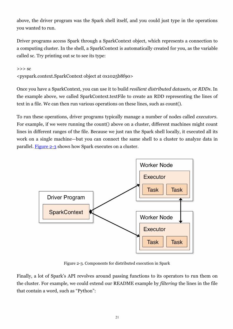
To run these operations, driver programs typically manage a number of nodes called executors.
For example, if we were running the count() above on a cluster, different machines might count
lines in different ranges of the file. Because we just ran the Spark shell locally, it executed all its
work on a single machine—but you can connect the same shell to a cluster to analyze data in
parallel. Figure 2-3 shows how Spark executes on a cluster.
Figure 2-3. Components for distributed execution in Spark
Finally, a lot of Spark’s API revolves around passing functions to its operators to run them on
the cluster. For example, we could extend our README example by filtering the lines in the file
that contain a word, such as “Python”:

22
Example 2-3. Python filtering example
>>> lines = sc.textFile("README.md")
>>> pythonLines = lines.filter(lambda line: "Python" in line)
>>> pythonLines.first()
u'## Interactive Python Shell'
Example 2-4. Scala filtering example
scala> val lines = sc.textFile("README.md") // Create an RDD called lines
lines: spark.RDD[String] = MappedRDD[...]
scala> val pythonLines = lines.filter(line => line.contains("Python"))
pythonLines: spark.RDD[String] = FilteredRDD[...]
scala> lines.first()
res0: String = ## Interactive Python Shell
Note
If you are unfamiliar with the lambda or => syntax above, it is a shorthand way to define
functions inline in Python and Scala. When using Spark in these languages, you can also define a
function separately and then pass its name to Spark. For example, in Python:
def hasPython(line):
return "Python" in line
pythonLines = lines.filter(hasPython)
Passing functions to Spark is also possible in Java, but in this case they are defined as classes,
implementing an interface called Function. For example:
JavaRDD<String> pythonLines = lines.filter(
new Function<String, Boolean>() {
Boolean call(String line) { return line.contains("Python"); }
}
);
Java 8 introduces shorthand syntax called “lambdas” that looks similar to Python and Scala.
Here is how the code would look with this syntax:
23
JavaRDD<String> pythonLines = lines.filter(line -> line.contains("Python"));
We discuss passing functions further in Passing Functions to Spark.
While we will cover the Spark API in more detail later, a lot of its magic is that function-based
operations like filter also parallelize across the cluster. That is, Spark automatically takes your
function (e.g. line.contains("Python")) and ships it to executor nodes. Thus, you can write code
in a single driver program and automatically have parts of it run on multiple nodes. Chapter 3
covers the RDD API in more detail.
Standalone Applications
The final piece missing in this quick tour of Spark is how to use it in standalone programs. Apart
from running interactively, Spark can be linked into standalone applications in either Java,
Scala or Python. The main difference from using it in the shell is that you need to initialize your
own SparkContext. After that, the API is the same.
The process of linking to Spark varies by language. In Java and Scala, you give your application
a Maven dependency on the spark-core artifact published by Apache. As of the time of writing,
the latest Spark version is 1.0.0, and the Maven coordinates for that are:
groupId = org.apache.spark
artifactId = spark-core_2.10
version = 1.0.0
If you are unfamiliar with Maven, it is a popular package management tool for Java-based
languages that lets you link to libraries in public repositories. You can use Maven itself to build
your project, or use other tools that can talk to the Maven repositories, including Scala’s SBT
tool or Gradle. Popular integrated development environments like Eclipse also allow you to
directly add a Maven dependency to a project.
In Python, you simply write applications as Python scripts, but you must instead run them using
a special bin/spark-submit script included in Spark. This script sets up the environment for
Spark’s Python API to function. Simply run your script with:
bin/spark-submit my_script.py
(Note that you will have to use backslashes instead of forward slashes on Windows.)

24
Note
In Spark versions before 1.0, use bin/pyspark my_script.py to run Python applications instead.
For detailed examples of linking applications to Spark, refer to the Quick Start Guide [6] in the
official Spark documentation. In a final version of the book, we will also include full examples in
an appendix.
Initializing a SparkContext
Once you have linked an application to Spark, you need to import the Spark packages in your
program and create a SparkContext. This is done by first creating a SparkConf object to
configure your application, and then building a SparkContext for it. Here is a short example in
each supported language:
Example 2-5. Initializing Spark in Python
from pyspark import SparkConf, SparkContext
conf = SparkConf().setMaster("local").setAppName("My App")
sc = SparkContext(conf)
Example 2-6. Initializing Spark in Java
import org.apache.spark.SparkConf;
import org.apache.spark.api.java.JavaSparkContext;
SparkConf conf = new SparkConf().setMaster("local").setAppName("My App");
JavaSparkContext sc = new JavaSparkContext(conf);
Example 2-7. Initializing Spark in Scala
import org.apache.spark.SparkConf
import org.apache.spark.SparkContext
import org.apache.spark.SparkContext._
val conf = new SparkConf().setMaster("local").setAppName("My App")
val sc = new SparkContext("local", "My App")
These examples show the minimal way to initialize a SparkContext, where you pass two
parameters:
A cluster URL, namely “local” in these examples, which tells Spark how to connect to a cluster. “local”
is a special value that runs Spark on one thread on the local machine, without connecting to a cluster.
25
An application name, namely “My App” in these examples. This will identify your application on the
cluster manager’s UI if you connect to a cluster.
Additional parameters exist for configuring how your application executes or adding code to be
shipped to the cluster, but we will cover these in later chapters of the book.
After you have initialized a SparkContext, you can use all the methods we showed before to
create RDDs (e.g. from a text file) and manipulate them.
Finally, to shut down Spark, you can either call the stop() method on your SparkContext, or
simply exit the application (e.g. with System.exit(0) or sys.exit()).
This quick overview should be enough to let you run a standalone Spark application on your
laptop. For more advanced configuration, a later chapter in the book will cover how to connect
your application to a cluster, including packaging your application so that its code is
automatically shipped to worker nodes. For now, please refer to the Quick Start Guide [7] in the
official Spark documentation.
Conclusion
In this chapter, we have covered downloading Spark, running it locally on your laptop, and
using it either interactively or from a standalone application. We gave a quick overview of the
core concepts involved in programming with Spark: a driver program creates a SparkContext
and RDDs, and then runs parallel operations on them. In the next chapter, we will dive more
deeply into how RDDs operate.
[5]http://spark.apache.org/docs/latest/quick-start.html
[6]http://spark.apache.org/docs/latest/quick-start.html
[7]http://spark.apache.org/docs/latest/quick-start.html

26
Chapter 3. Programming with RDDs
This chapter introduces Spark’s core abstraction for working with data, the Resilient Distributed
Dataset (RDD). An RDD is simply a distributed collection of elements. In Spark all work is
expressed as either creating new RDDs, transforming existing RDDs, or calling operations on
RDDs to compute a result. Under the hood, Spark automatically distributes the data contained
in RDDs across your cluster and parallelizes the operations you perform on them.
Both Data Scientists and Engineers should read this chapter, as RDDs are the core concept in
Spark. We highly recommend that you try some of these examples in an interactive shell (see
Introduction to Spark’s Python and Scala Shells). In addition, all code in this chapter is available
in the book’s GitHub repository.
RDD Basics
An RDD in Spark is simply a distributed collection of objects. Each RDD is split into multiple
partitions, which may be computed on different nodes of the cluster. RDDs can contain any type
of Python, Java or Scala objects, including user-defined classes.
Users create RDDs in two ways: by loading an external dataset, or by distributing a collection of
objects in their driver program. We have already seen loading a text file as an RDD of strings
using SparkContext.textFile():
Example 3-1. Creating an RDD of strings with textFile() in Python
>>> lines = sc.textFile("README.md")
Once created, RDDs offer two types of operations: transformations and actions.
Transformations construct a new RDD from a previous one. For example, one transformation
we saw before is filtering data that matches a predicate. In our text file example, we can use this
to create a new RDD holding just the strings that contain “Python”:
>>> pythonLines = lines.filter(lambda line: "Python" in line)
Actions, on the other hand, compute a result based on an RDD, and either return it to the driver
program or save it to an external storage system (e.g., HDFS). One example of an action we
called earlier is first(), which returns the first element in an RDD:
>>> pythonLines.first()

27
u'## Interactive Python Shell'
The difference between transformations and actions is due to the way Spark computes RDDs.
Although you can define new RDDs any time, Spark only computes them in a lazy fashion, the
first time they are used in an action. This approach might seem unusual at first, but makes a lot
of sense when working with big data. For instance, consider the example above, where we
defined a text file and then filtered the lines with “Python”. If Spark were to load and store all
the lines in the file as soon as we wrote lines = sc.textFile(...), it would waste a lot of storage
space, given that we then immediately filter out many lines. Instead, once Spark sees the whole
chain of transformations, it can compute just the data needed for its result. In fact, for the first()
action, Spark only scans the file until it finds the first matching line; it doesn’t even read the
whole file.
Finally, Spark’s RDDs are by default recomputed each time you run an action on them. If you
would like to reuse an RDD in multiple actions, you can ask Spark to persist it using
RDD.persist(). After computing it the first time, Spark will store the RDD contents in memory
(partitioned across the machines in your cluster), and reuse them in future actions. Persisting
RDDs on disk instead of memory is also possible. The behavior of not persisting by default may
again seem unusual, but it makes a lot of sense for big datasets: if you will not reuse the RDD,
there’s no reason to waste storage space when Spark could instead stream through the data once
and just compute the result.[8]
In practice, you will often use persist to load a subset of your data into memory and query it
repeatedly. For example, if we knew that we wanted to compute multiple results about the
README lines that contain “Python”, we could write:
>>> pythonLines.persist()
>>> pythonLines.count()
2
>>> pythonLines.first()
u'## Interactive Python Shell'
To summarize, every Spark program and shell session will work as follows:
1. Create some input RDDs from external data.
2. Transform them to define new RDDs using transformations like filter().
3. Ask Spark to persist() any intermediate RDDs that will need to be reused.

28
4. Launch actions such as count() and first() to kick off a parallel computation, which is then optimized
and executed by Spark.
In the rest of this chapter, we’ll go through each of these steps in detail, and cover some of the
most common RDD operations in Spark.
Creating RDDs
Spark provides two ways to create RDDs: loading an external dataset and parallelizing a
collection in your driver program.
The simplest way to create RDDs is to take an existing in-memory collection and pass it to
SparkContext’s parallelize method. This approach is very useful when learning Spark, since you
can quickly create your own RDDs in the shell and perform operations on them. Keep in mind
however, that outside of prototyping and testing, this is not widely used since it requires you
have your entire dataset in memory on one machine.
Example 3-2. Python parallelize example
lines = sc.parallelize(["pandas", "i like pandas"])
Example 3-3. Scala parallelize example
val lines = sc.parallelize(List("pandas", "i like pandas"))
Example 3-4. Java parallelize example
JavaRDD<String> lines = sc.parallelize(Arrays.asList("pandas", "i like pandas"));
A more common way to create RDDs is to load data in external storage. Loading external
datasets is covered in detail in Chapter 5. However, we already saw one method that loads a text
file as an RDD of strings, SparkContext.textFile:
Example 3-5. Python textFile example
lines = sc.textFile("/path/to/README.md")
Example 3-6. Scala textFile example
val lines = sc.textFile("/path/to/README.md")
Example 3-7. Java textFile example
JavaRDD<String> lines = sc.textFile("/path/to/README.md");
RDD Operations
RDDs support two types of operations, transformations and actions. Transformations are
operations on RDDs that return a new RDD, such as map and filter. Actions are operations that
return a result back to the driver program or write it to storage, and kick off a computation, such
29
as count and first. Spark treats transformations and actions very differently, so understanding
which type of operation you are performing will be important. If you are ever confused whether
a given function is a transformation or and action, you can look at its return type:
transformations return RDDs whereas actions return some other data type.
Transformations
Transformations are operations on RDDs that return a new RDD. As discussed in the lazy
evaluation section, transformed RDDs are computed lazily, only when you use them in an action.
Many transformations are element-wise, that is they work on one element at a time, but this is
not true for all transformations.
As an example, suppose that we have a log file, log.txt, with a number of messages, and we want
to select only the error messages. We can use the filter transformation seen before. This time
though, we’ll show a filter in all three of Spark’s language APIs:
Example 3-8. Python filter example
inputRDD = sc.textFile("log.txt")
errorsRDD = inputRDD.filter(lambda x: "error" in x)
Example 3-9. Scala filter example
val inputRDD = sc.textFile("log.txt")
val errorsRDD = inputRDD.filter(line => line.contains("error"))
Example 3-10. Java filter example
JavaRDD<String> inputRDD = sc.textFile("log.txt");
JavaRDD<String> errorsRDD = inputRDD.filter(
new Function<String, Boolean>() {
public Boolean call(String x) { return x.contains("error");
}
});
Note that the filter operation does not mutate the existing inputRDD. Instead, it returns a
pointer to an entirely new RDD. inputRDD can still be re-used later in the program, for instance,
to search for other words. In fact, let’s use inputRDD again to search for lines with the word
“warning” in them. Then, we’ll use another transformation, union, to print out the number of
lines that contained either “error” or “warning”. We show Python here, but the union() function
is identical in all three languages:
Example 3-11. Python union example
errorsRDD = inputRDD.filter(lambda x: "error" in x)
warningsRDD = inputRDD.filter(lambda x: "warning" in x)
30
badLinesRDD = errorsRDD.union(warningsRDD)
union is a bit different than filter, in that it operates on two RDDs instead of one.
Transformations can actually operate on any number of input RDDs.
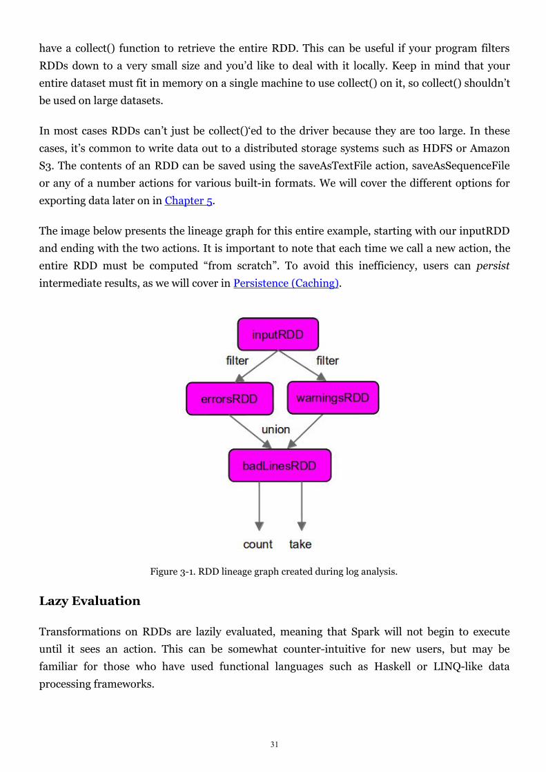
Finally, as you derive new RDDs from each other using transformations, Spark keeps track of
the set of dependencies between different RDDs, called the lineage graph. It uses this
information to compute each RDD on demand and to recover lost data if part of a persistent
RDD is lost. We will show a lineage graph for this example in Figure 3-1.
Actions
We’ve seen how to create RDDs from each other with transformations, but at some point, we’ll
want to actually do something with our dataset. Actions are the second type of RDD operation.
They are the operations that return a final value to the driver program or write data to an
external storage system. Actions force the evaluation of the transformations required for the
RDD they are called on, since they are required to actually produce output.
Continuing the log example from the previous section, we might want to print out some
information about the badLinesRDD. To do that, we’ll use two actions, count(), which returns
the count as a number, and take(), which collects a number of elements from the RDD.
Example 3-12. Python error count example using actions
print "Input had " + badLinesRDD.count() + " concerning lines"
print "Here are 10 examples:"
for line in badLinesRDD.take(10):
print line
Example 3-13. Scala error count example using actions
println("Input had " + badLinesRDD.count() + " concerning lines")
println("Here are 10 examples:")
badLinesRDD.take(10).foreach(println)
Example 3-14. Java error count example using actions
System.out.println("Input had " + badLinesRDD.count() + " concerning lines")
System.out.println("Here are 10 examples:")
for (String line: badLinesRDD.take(10)) {
System.out.println(line);
}
In this example, we used take() to retrieve a small number of elements in the RDD at the driver
program. We then iterate over them locally to print out information at the driver. RDDs also
31
have a collect() function to retrieve the entire RDD. This can be useful if your program filters
RDDs down to a very small size and you’d like to deal with it locally. Keep in mind that your
entire dataset must fit in memory on a single machine to use collect() on it, so collect() shouldn’t
be used on large datasets.
In most cases RDDs can’t just be collect()‘ed to the driver because they are too large. In these
cases, it’s common to write data out to a distributed storage systems such as HDFS or Amazon
S3. The contents of an RDD can be saved using the saveAsTextFile action, saveAsSequenceFile
or any of a number actions for various built-in formats. We will cover the different options for
exporting data later on in Chapter 5.
The image below presents the lineage graph for this entire example, starting with our inputRDD
and ending with the two actions. It is important to note that each time we call a new action, the
entire RDD must be computed “from scratch”. To avoid this inefficiency, users can persist
intermediate results, as we will cover in Persistence (Caching).
Figure 3-1. RDD lineage graph created during log analysis.
Lazy Evaluation
Transformations on RDDs are lazily evaluated, meaning that Spark will not begin to execute
until it sees an action. This can be somewhat counter-intuitive for new users, but may be
familiar for those who have used functional languages such as Haskell or LINQ-like data
processing frameworks.

32
Lazy evaluation means that when we call a transformation on an RDD (for instance calling map),
the operation is not immediately performed. Instead, Spark internally records meta-data to
indicate this operation has been requested. Rather than thinking of an RDD as containing
specific data, it is best to think of each RDD as consisting of instructions on how to compute the
data that we build up through transformations. Loading data into an RDD is lazily evaluated in
the same way transformations are. So when we call sc.textFile the data is not loaded until it is
necessary. Like with transformations, the operation (in this case reading the data) can occur
multiple times.
Tip
Although transformations are lazy, force Spark to execute them at any time by running an action,
such as count(). This is an easy way to test out just part of your program.
Spark uses lazy evaluation to reduce the number of passes it has to take over our data by
grouping operations together. In MapReduce systems like Hadoop, developers often have to
spend a lot time considering how to group together operations to minimize the number of
MapReduce passes. In Spark, there is no substantial benefit to writing a single complex map
instead of chaining together many simple operations. Thus, users are free to organize their
program into smaller, more manageable operations.
Passing Functions to Spark
Most of Spark transformations, and some of its actions, depend on passing in functions that are
used by Spark to compute data. Each of the core languages has a slightly different mechanism
for passing functions to Spark.
Python
In Python, we have three options for passing functions into Spark. For shorter function we can
pass in lambda expressions, as we have done in the example at the start of this chapter. We can
also pass in top-level functions, or locally defined functions.
Example 3-15. Passing a lambda in Python
word = rdd.filter(lambda s: "error" in s)
Passing a top-level Python function.
def containsError(s):
return "error" in s
33
word = rdd.filter(containsError)
One issue to watch out for when passing functions if that if you pass functions that are members
of an object, or references to fields in an object (e.g., self.field), this results in sending in the
entire object, which can be much larger than just the bit of information you need. Sometimes
this can also cause your program to fail, if your class contains objects that Python can’t figure
out how to pickle.
Example 3-16. Passing a function with field references (don’t do this!)
class SearchFunctions(object):
def __init__(self, query):
self.query = query
def isMatch(self, s):
return query in s
def getMatchesFunctionReference(self, rdd):
# Problem: references all of "self" in "self.isMatch"
return rdd.filter(self.isMatch)
def getMatchesMemberReference(self, rdd):
# Problem: references all of "self" in "self.query"
return rdd.filter(lambda x: self.query in x)
Instead, just extract the fields you need from your object into local variable and pass that in, like
we do below:
Example 3-17. Python function passing without field references
class WordFunctions(object):
...
def getMatchesNoReference(self, rdd):
# Safe: extract only the field we need into a local variable
query = self.query
return rdd.filter(lambda x: query in x)
Scala
In Scala, we can pass in functions defined inline or references to methods or static functions as
we do for Scala’s other functional APIs. Some other considerations come into play though,
namely that the function we pass and the data referenced in it needs to be Serializable
(implementing Java’s Serializable interface). Furthermore, like in Python, passing a method or
field of an object includes a reference to that whole object, though this is less obvious because
we are not forced to write these references with self. Like how we did with Python, we can

34
instead extract out the fields we need as local variables and avoid needing to pass the whole
object containing them.
Example 3-18. Scala function passing
class SearchFunctions(val query: String) {
def isMatch(s: String): Boolean = {
s.contains(query)
}
def getMatchesFunctionReference(rdd: RDD[String]): RDD[String] = {
// Problem: "isMatch" means "this.isMatch", so we pass all of "this"
rdd.map(isMatch)
}
def getMatchesFieldReference(rdd: RDD[String]): RDD[String] = {
// Problem: "query" means "this.query", so we pass all of "this"
rdd.map(x => x.split(query))
}
def getMatchesNoReference(rdd: RDD[String]): RDD[String] = {
// Safe: extract just the field we need into a local variable
val query_ = this.query
rdd.map(x => x.split(query_))
}
}
If you “NotSerializableException” errors in Scala, a reference to a method or field in a
non-serializable class is usually the problem. Note that passing in local variables or functions
that are members of a top-level object is always safe.
Java
In Java, functions are specified as objects that implement one of Spark’s function interfaces
from the org.apache.spark.api.java.function package. There are a number of different interfaces
based on the return type of the function. We show the most basic function interfaces below, and
cover a number of other function interfaces for when we need to return special types of data in
the section on converting between RDD types.
35
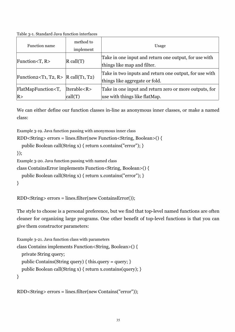
Table 3-1. Standard Java function interfaces
Function namemethod to
implementUsage
Function<T, R> R call(T)Take in one input and return one output, for use with
things like map and filter.
Function2<T1, T2, R> R call(T1, T2)Take in two inputs and return one output, for use with
things like aggregate or fold.
FlatMapFunction<T,
R>
Iterable<R>
call(T)
Take in one input and return zero or more outputs, for
use with things like flatMap.
We can either define our function classes in-line as anonymous inner classes, or make a named
class:
Example 3-19. Java function passing with anonymous inner class
RDD<String> errors = lines.filter(new Function<String, Boolean>() {
public Boolean call(String x) { return s.contains("error"); }
});
Example 3-20. Java function passing with named class
class ContainsError implements Function<String, Boolean>() {
public Boolean call(String x) { return x.contains("error"); }
}
RDD<String> errors = lines.filter(new ContainsError());
The style to choose is a personal preference, but we find that top-level named functions are often
cleaner for organizing large programs. One other benefit of top-level functions is that you can
give them constructor parameters:
Example 3-21. Java function class with parameters
class Contains implements Function<String, Boolean>() {
private String query;
public Contains(String query) { this.query = query; }
public Boolean call(String x) { return x.contains(query); }
}
RDD<String> errors = lines.filter(new Contains("error"));

36
In Java 8, you can also use lambda expressions to concisely implement the Function interfaces.
Since Java 8 is still relatively new as of the writing of this book, our examples use the more
verbose syntax for defining classes in previous versions of Java. However, with lambda
expressions, our search example would look like this:
Example 3-22. Java function passing with lambda expression in Java 8
RDD<String> errors = lines.filter(s -> s.contains("error"));
If you are interested in using Java 8’s lambda expression, refer to Oracle’s documentation and
the Databricks blog post on how to use lambdas with Spark.
Tip
Both anonymous inner classes and lambda expressions can reference any final variables in the
method enclosing them, so you can pass these variables to Spark just like in Python and Scala.
Common Transformations and Actions
In this chapter, we tour the most common transformations and actions in Spark. Additional
operations are available on RDDs containing certain type of data—for example, statistical
functions on RDDs of numbers, and key-value operations such as aggregating data by key on
RDDs of key-value pairs. We cover converting between RDD types and these special operations
in later sections.
Basic RDDs
We will begin by evaluating what operations we can do on all RDDs regardless of the data. These
transformations and actions are available on all RDD classes.
Transformations
Element-wise transformations
The two most common transformations you will likely be performing on basic RDDs are map,
and filter. The map transformation takes in a function and applies it to each element in the RDD
with the result of the function being the new value of each element in the resulting RDD. The
filter transformation take in a function and returns an RDD which only has elements that pass
the filter function.
37
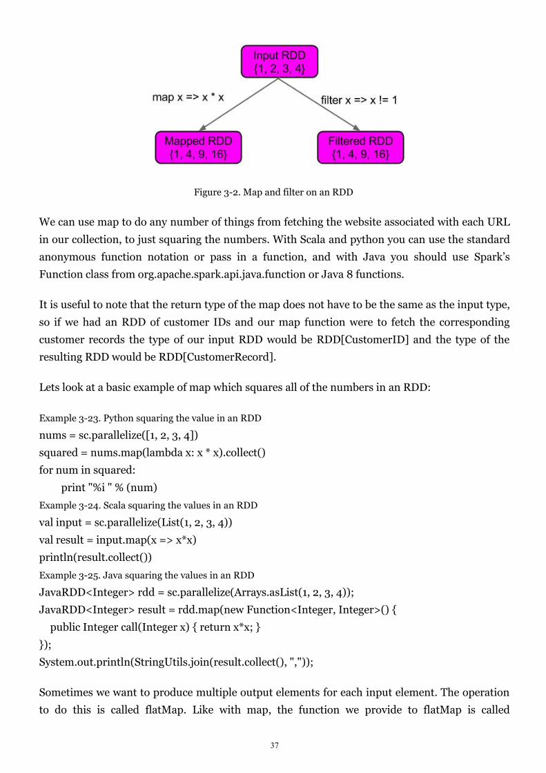
Figure 3-2. Map and filter on an RDD
We can use map to do any number of things from fetching the website associated with each URL
in our collection, to just squaring the numbers. With Scala and python you can use the standard
anonymous function notation or pass in a function, and with Java you should use Spark’s
Function class from org.apache.spark.api.java.function or Java 8 functions.
It is useful to note that the return type of the map does not have to be the same as the input type,
so if we had an RDD of customer IDs and our map function were to fetch the corresponding
customer records the type of our input RDD would be RDD[CustomerID] and the type of the
resulting RDD would be RDD[CustomerRecord].
Lets look at a basic example of map which squares all of the numbers in an RDD:
Example 3-23. Python squaring the value in an RDD
nums = sc.parallelize([1, 2, 3, 4])
squared = nums.map(lambda x: x * x).collect()
for num in squared:
print "%i " % (num)
Example 3-24. Scala squaring the values in an RDD
val input = sc.parallelize(List(1, 2, 3, 4))
val result = input.map(x => x*x)
println(result.collect())
Example 3-25. Java squaring the values in an RDD
JavaRDD<Integer> rdd = sc.parallelize(Arrays.asList(1, 2, 3, 4));
JavaRDD<Integer> result = rdd.map(new Function<Integer, Integer>() {
public Integer call(Integer x) { return x*x; }
});
System.out.println(StringUtils.join(result.collect(), ","));
Sometimes we want to produce multiple output elements for each input element. The operation
to do this is called flatMap. Like with map, the function we provide to flatMap is called
38
individually for each element in our input RDD. Instead of returning a single element, we return
an iterator with our return values. Rather than producing an RDD of iterators, we get back an
RDD which consists of the elements from all of the iterators. A simple example of flatMap is
splitting up an input string into words, as shown below.
Example 3-26. Python flatMap example, splitting lines into words
lines = sc.parallelize(["hello world", "hi"])
words = lines.flatMap(lambda line: line.split(" "))
words.first() # returns "hello"
Example 3-27. Scala flatMap example, splitting lines into multiple words
val lines = sc.parallelize(List("hello world", "hi"))
val words = lines.flatMap(line => line.split(" "))
words.first() // returns "hello"
Example 3-28. Scala flatMap example, splitting lines into multiple words
JavaRDD<String> lines = sc.parallelize(Arrays.asList("hello world", "hi"));
JavaRDD<String> words = rdd.flatMap(new FlatMapFunction<String, String>() {
public Iterable<String> call(String line) {
return Arrays.asList(line.split(" "));
}
});
words.first(); // returns "hello"
Pseudo Set Operations
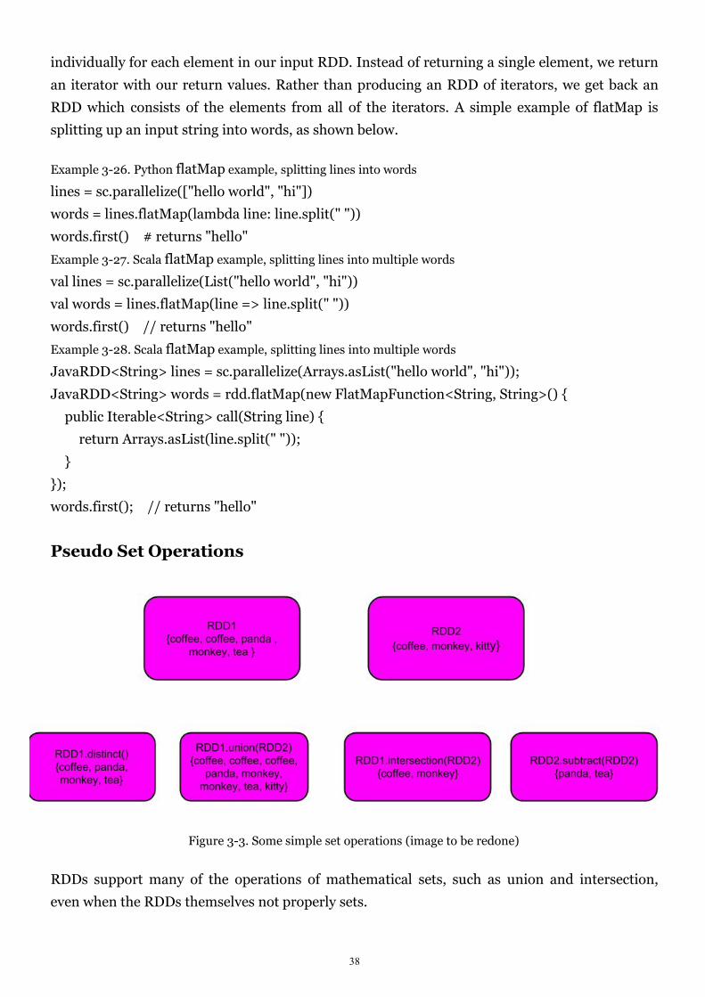
Figure 3-3. Some simple set operations (image to be redone)
RDDs support many of the operations of mathematical sets, such as union and intersection,
even when the RDDs themselves not properly sets.
39
The set property most frequently missing from our RDDs is the uniqueness of elements. If we
only want unique elements we can use the RDD.distinct() transformation to produce a new RDD
with only distinct items. Note that distinct() is expensive, however, as it requires shuffling all the
data over the network to ensure that we only receive one copy of each element.
The simplest set operation is union(other), which gives back an RDD consisting of the data from
both sources. This can be useful in a number of use cases, such as processing log files from many
sources. Unlike the mathematical union(), if there are duplicates in the input RDDs, the result of
Spark’s union() will contain duplicates (which we can fix if desired with distinct()).
Spark also provides an intersection(other) method, which returns only elements in both RDDs.
intersection() also removes all duplicates (including duplicates from a single RDD) while
running. While intersection and union are to very similar concepts, the performance of
intersection is much worse since it requires a shuffle over the network to identify common
elements.
Sometimes we need to remove some data from consideration. The subtract(other) function takes
in another RDD and returns an RDD that only has values present in the first RDD and not the
second RDD.
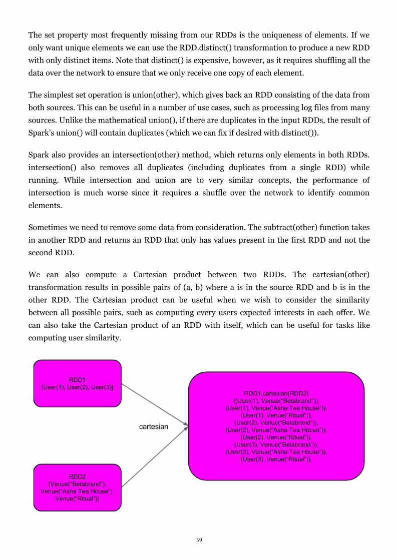
We can also compute a Cartesian product between two RDDs. The cartesian(other)
transformation results in possible pairs of (a, b) where a is in the source RDD and b is in the
other RDD. The Cartesian product can be useful when we wish to consider the similarity
between all possible pairs, such as computing every users expected interests in each offer. We
can also take the Cartesian product of an RDD with itself, which can be useful for tasks like
computing user similarity.

40
Figure 3-4. Cartesian product between two RDDs
The tables below summarize common single-RDD and multi-RDD transformations.
Table 3-2. Basic RDD transformations on an RDD containing {1, 2, 3, 3}
Function Name Purpose Example Result
map
Apply a function to each
element in the RDD and
return an RDD of the result
rdd.map(x => x +
1){2, 3, 4, 4}
flatMap
Apply a function to each
element in the RDD and
return an RDD of the
contents of the iterators
returned. Often used to
extract words.
rdd.flatMap(x =>
x.to(3)){1, 2, 3, 2, 3, 3, 3}
filter
Return an RDD consisting of
only elements which pass the
condition passed to filter
rdd.filter(x =>
x != 1){2, 3, 3}
distinct Remove duplicates rdd.distinct() {1, 2, 3}
sample(withReplacement,
fraction, [seed])Sample an RDD
rdd.sample(false,
0.5)non-deterministic
Table 3-3. Two-RDD transformations on RDDs containing {1, 2, 3} and {3, 4, 5}
Function
NamePurpose Example Result
unionProduce an RDD contain elements from
both RDDsrdd.union(other) {1, 2, 3, 3, 4, 5}
intersectionRDD containing only elements found in
both RDDsrdd.intersection(other) {3}
subtractRemove the contents of one RDD (e.g.
remove training data)rdd.subtract(other) {1, 2}
cartesian Cartesian product with the other RDD rdd.cartesian(other){(1, 3), (1, 4), …
(3,5)}
As you can see there are a wide variety of transformations available on all RDDs regardless of
our specific underlying data. We can transform our data element-wise, obtain distinct elements,
and do a variety of set operations.

41
Actions
The most common action on basic RDDs you will likely use is reduce. Reduce takes in a function
which operates on two elements of the same type of your RDD and returns a new element of the
same type. A simple example of such a function is + , which we can use to sum our RDD. With
reduce we can easily sum the elements of our RDD, count the number of elements, and perform
other types of aggregations.
Example 3-29. Python reduce example
sum = rdd.reduce(lambda x, y: x + y)
Example 3-30. Scala reduce example
val sum = rdd.reduce((x, y) => x + y)
Example 3-31. Java reduce example
Integer sum = rdd.reduce(new Function2<Integer, Integer, Integer>() {
public Integer call(Integer x, Integer y) { return x + y;}
});
Similar to reduce is fold which also takes a function with the same signature as needed for
reduce, but also takes a “zero value” to be used for the initial call on each partition. The zero
value you provide should be the identity element for your operation, that is applying it multiple
times with your function should not change the value, (e.g. 0 for +, 1 for *, or an empty list for
concatenation).
Tip
You can minimize object creation in fold by modifying and returning the first of the two
parameters in-place. However, you should not modify the second parameter.
Fold and reduce both require that the return type of our result be the same type as that of the
RDD we are operating over. This works well for doing things like sum, but sometimes we want
to return a different type. For example when computing the running average we need to have a
different return type. We could implement this using a map first where we transform every
element into the element and the number 1 so that the reduce function can work on pairs.
The aggregate function frees us from the constraint of having the return the same type as the
RDD which we are working on. With aggregate, like fold, we supply an initial zero value of the
type we want to return. We then supply a function to combine the elements from our RDD with
the accumulator. Finally, we need to supply a second function to merge two accumulators, given
that each node accumulates its own results locally.
42
We can use aggregate to compute the average of a RDD avoiding a map before the fold.
Example 3-32. Python aggregate example
sumCount = nums.aggregate((0, 0),
(lambda x, y: (x[0] + y, x[1] + 1),
(lambda x, y: (x[0] + y[0], x[1] + y[1]))))
return sumCount[0] / float(sumCount[1])
Example 3-33. Scala aggregate example
val result = input.aggregate((0, 0))(
(x, y) => (x._1 + y, x._2 + 1),
(x, y) => (x._1 + y._1, x._2 + y._2))
val avg = result._1 / result._2.toDouble
Example 3-34. Java aggregate example
class AvgCount {
public AvgCount(int total, int num) {
this.total = total;
this.num = num;
}
public int total;
public int num;
public double avg() {
return total / (double) num;
}
}
Function2<AvgCount, Integer, AvgCount> addAndCount =
new Function2<AvgCount, Integer, AvgCount>() {
public AvgCount call(AvgCount a, Integer x) {
a.total += x;
a.num += 1;
return a;
}
};
Function2<AvgCount, AvgCount, AvgCount> combine =
new Function2<AvgCount, AvgCount, AvgCount>() {
public AvgCount call(AvgCount a, AvgCount b) {
a.total += b.total;
a.num += b.num;
return a;
}
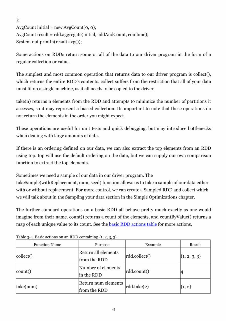
43
};
AvgCount initial = new AvgCount(0, 0);
AvgCount result = rdd.aggregate(initial, addAndCount, combine);
System.out.println(result.avg());
Some actions on RDDs return some or all of the data to our driver program in the form of a
regular collection or value.
The simplest and most common operation that returns data to our driver program is collect(),
which returns the entire RDD’s contents. collect suffers from the restriction that all of your data
must fit on a single machine, as it all needs to be copied to the driver.
take(n) returns n elements from the RDD and attempts to minimize the number of partitions it
accesses, so it may represent a biased collection. Its important to note that these operations do
not return the elements in the order you might expect.
These operations are useful for unit tests and quick debugging, but may introduce bottlenecks
when dealing with large amounts of data.
If there is an ordering defined on our data, we can also extract the top elements from an RDD
using top. top will use the default ordering on the data, but we can supply our own comparison
function to extract the top elements.
Sometimes we need a sample of our data in our driver program. The
takeSample(withReplacement, num, seed) function allows us to take a sample of our data either
with or without replacement. For more control, we can create a Sampled RDD and collect which
we will talk about in the Sampling your data section in the Simple Optimizations chapter.
The further standard operations on a basic RDD all behave pretty much exactly as one would
imagine from their name. count() returns a count of the elements, and countByValue() returns a
map of each unique value to its count. See the basic RDD actions table for more actions.
Table 3-4. Basic actions on an RDD containing {1, 2, 3, 3}
Function Name Purpose Example Result
collect()Return all elements
from the RDDrdd.collect() {1, 2, 3, 3}
count()Number of elements
in the RDDrdd.count() 4
take(num)Return num elements
from the RDDrdd.take(2) {1, 2}

44
Function Name Purpose Example Result
top(num)Return the top num
elements the RDDrdd.top(2) {3, 3}
takeOrdered(num)(ordering)
Return num elements
based on providing
ordering
rdd.takeOrdered(2)(myOr
dering){3, 3}
takeSample(withReplacement,
num, [seed])
Return num elements
at randomrdd.takeSample(false, 1)
non-determini
stic
reduce(func)
Combine the elements
of the RDD together in
parallel (e.g. sum)
rdd.fold((x, y) => x + y) 9
fold(zero)(func)
Same as reduce but
with the provided zero
value
rdd.fold(0)((x, y) => x + y) 9
aggregate(zeroValue)(seqOp,
combOp)
Similar to reduce but
used to return a
different type
rdd.aggregate(0, 0) ({case
(x, y) => (y._1() + x, y._2()
+ 1)}, {case (x, y) =>
(y._1() + x._1(), y._2() +
x._2()) })
(9, 4)
foreach(func)
Apply the provided
function to each
element of the RDD
rdd.foreach(func) nothing
Converting Between RDD Types
We don’t have to do anything special to get back the correct templated/generic type of RDD
(that is, our RDD of Strings can become an RDD of Integers just by calling map with the correct
function). Some functions are only available on certain types of RDDs, such as average on
numeric RDDs and join on key-value pair RDDs. We will cover these special functions for
numeric data in (to come) and pair RDDs in Chapter 4.
In Scala and Java, these methods aren’t defined on the standard RDD class, so to access this
additional functionality we have to make sure we get the correct specialized class.
Scala
In Scala the conversion between such RDDs (like from RDD[Double] and RDD[Numeric] to
DoubleRDD) is handled automatically using implicit conversions. A mentioned in standard
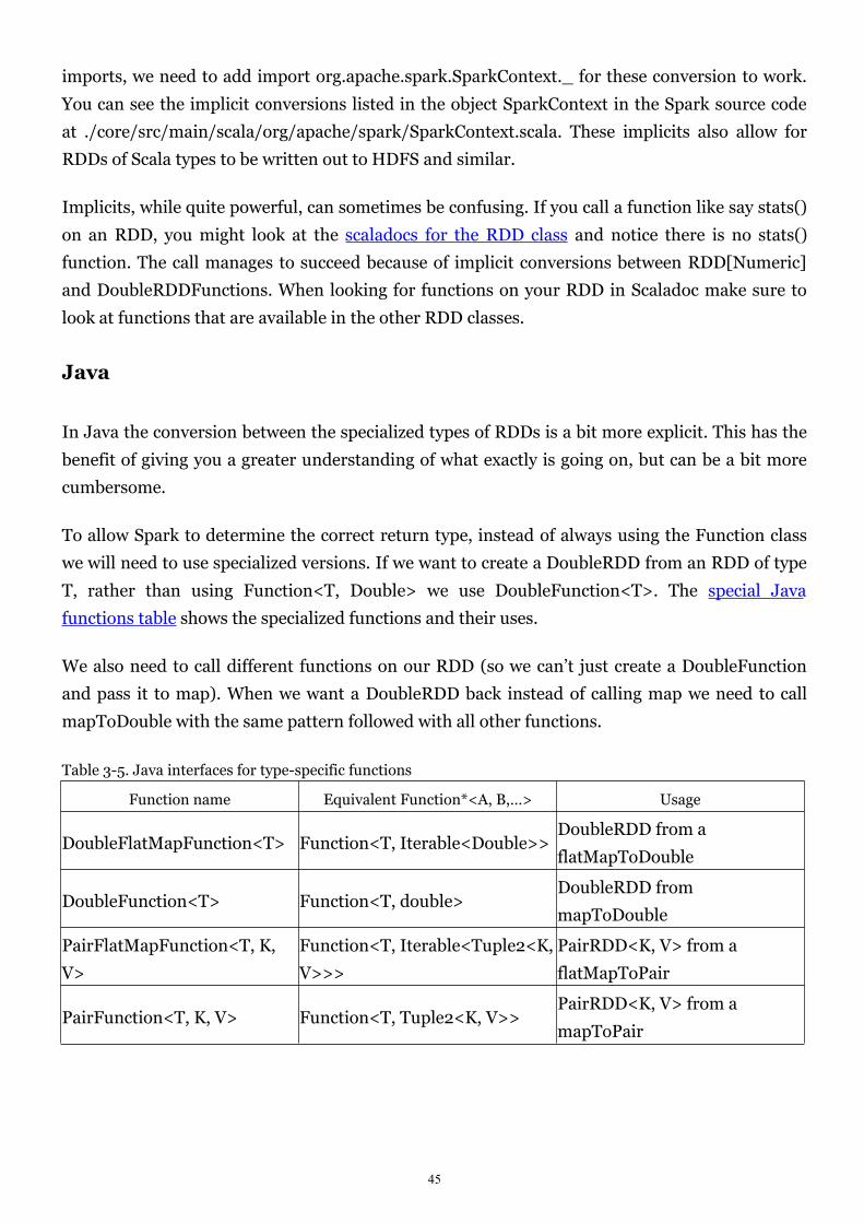
45
imports, we need to add import org.apache.spark.SparkContext._ for these conversion to work.
You can see the implicit conversions listed in the object SparkContext in the Spark source code
at ./core/src/main/scala/org/apache/spark/SparkContext.scala. These implicits also allow for
RDDs of Scala types to be written out to HDFS and similar.
Implicits, while quite powerful, can sometimes be confusing. If you call a function like say stats()
on an RDD, you might look at the scaladocs for the RDD class and notice there is no stats()
function. The call manages to succeed because of implicit conversions between RDD[Numeric]
and DoubleRDDFunctions. When looking for functions on your RDD in Scaladoc make sure to
look at functions that are available in the other RDD classes.
Java
In Java the conversion between the specialized types of RDDs is a bit more explicit. This has the
benefit of giving you a greater understanding of what exactly is going on, but can be a bit more
cumbersome.
To allow Spark to determine the correct return type, instead of always using the Function class
we will need to use specialized versions. If we want to create a DoubleRDD from an RDD of type
T, rather than using Function<T, Double> we use DoubleFunction<T>. The special Java
functions table shows the specialized functions and their uses.
We also need to call different functions on our RDD (so we can’t just create a DoubleFunction
and pass it to map). When we want a DoubleRDD back instead of calling map we need to call
mapToDouble with the same pattern followed with all other functions.
Table 3-5. Java interfaces for type-specific functions
Function name Equivalent Function*<A, B,…> Usage
DoubleFlatMapFunction<T> Function<T, Iterable<Double>>DoubleRDD from a
flatMapToDouble
DoubleFunction<T> Function<T, double>DoubleRDD from
mapToDouble
PairFlatMapFunction<T, K,
V>
Function<T, Iterable<Tuple2<K,
V>>>
PairRDD<K, V> from a
flatMapToPair
PairFunction<T, K, V> Function<T, Tuple2<K, V>>PairRDD<K, V> from a
mapToPair

46
We can modify our previous example where we squared an RDD of numbers to produce a
JavaDoubleRDD. This gives us access to the additional DoubleRDD specific functions like
average and stats.
Example 3-35. Java create DoubleRDD example
JavaDoubleRDD result = rdd.mapToDouble(
new DoubleFunction<Integer>() {
public double call(Integer x) {
return (double) x * x;
}
});
System.out.println(result.average());
Python
The Python API is structured a bit different than both the Java and Scala API. Like the Scala API,
we don’t need to be explicit to access the functions which are only available on Double or Pair
RDDs. In Python all of the functions are implemented on the base RDD class and will simply fail
at runtime if the type doesn’t work.
Persistence (Caching)
As discussed earlier, Spark RDDs are lazily evaluated, and sometimes we may wish to use the
same RDD multiple times. If we do this naively, Spark will recompute the RDD and all of its
dependencies each time we call an action on the RDD. This can be especially expensive for
iterative algorithms, which look at the data many times. Another trivial example would be doing
a count and then writing out the same RDD.
Example 3-36. Scala double execute example
val result = input.map(x => x*x)
println(result.count())
println(result.collect().mkString(","))
To avoid computing an RDD multiple times, we can ask Spark to persist the data. When we ask
Spark to persist an RDD, the nodes that compute the RDD store their partitions. If a node that
has data persisted on it fails, Spark will recompute the lost partitions of the data when needed.
We can also replicate our data on multiple nodes if we want to be able to handle node failure
without slowdown.
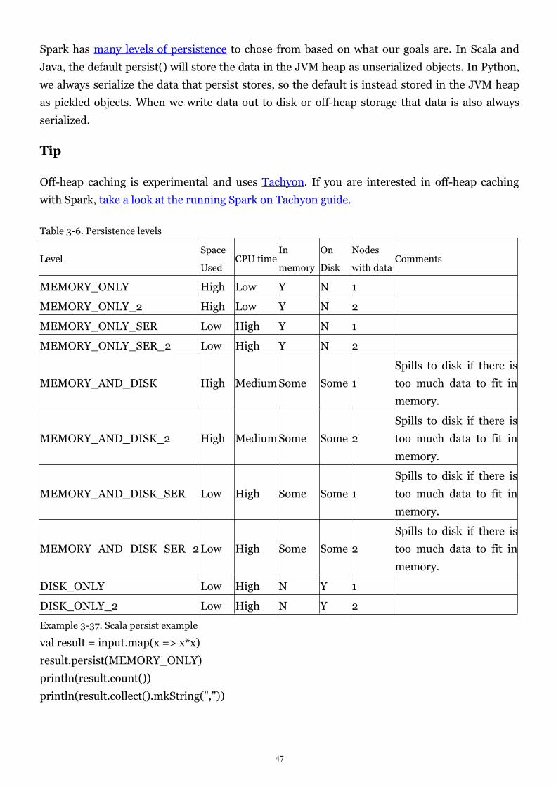
47
Spark has many levels of persistence to chose from based on what our goals are. In Scala and
Java, the default persist() will store the data in the JVM heap as unserialized objects. In Python,
we always serialize the data that persist stores, so the default is instead stored in the JVM heap
as pickled objects. When we write data out to disk or off-heap storage that data is also always
serialized.
Tip
Off-heap caching is experimental and uses Tachyon. If you are interested in off-heap caching
with Spark, take a look at the running Spark on Tachyon guide.
Table 3-6. Persistence levels
LevelSpace
UsedCPU time
In
memory
On
Disk
Nodes
with dataComments
MEMORY_ONLY High Low Y N 1
MEMORY_ONLY_2 High Low Y N 2
MEMORY_ONLY_SER Low High Y N 1
MEMORY_ONLY_SER_2 Low High Y N 2
MEMORY_AND_DISK High MediumSome Some 1
Spills to disk if there is
too much data to fit in
memory.
MEMORY_AND_DISK_2 High MediumSome Some 2
Spills to disk if there is
too much data to fit in
memory.
MEMORY_AND_DISK_SER Low High Some Some 1
Spills to disk if there is
too much data to fit in
memory.
MEMORY_AND_DISK_SER_2Low High Some Some 2
Spills to disk if there is
too much data to fit in
memory.
DISK_ONLY Low High N Y 1
DISK_ONLY_2 Low High N Y 2
Example 3-37. Scala persist example
val result = input.map(x => x*x)
result.persist(MEMORY_ONLY)
println(result.count())
println(result.collect().mkString(","))

48
Tip
You will note that we called persist on the RDD before the first action. The persist call on its own
doesn’t force evaluation.
If you attempt to cache too much data to fit in memory, Spark will automatically evict old
partitions using a Least Recently Used (LRU) cache policy. For the memory-only storage levels,
it will recompute these partitions the next time they are accessed, while for the
memory-and-disk ones, it will write them out to disk. In either case, this means that you don’t
have to worry about your job breaking if you ask Spark to cache too much data. However,
caching unnecessary data can lead to eviction of useful data and more recomputation time.
Finally, RDDs come with a method called unpersist() that lets you manually remove them from
the cache.
Conclusion
In this chapter, we have covered the RDD execution model and a large number of common
operations on RDDs. If you have gotten here, congratulations—you’ve learned all the core
concepts of working in Spark. In the next chapter, we’ll cover a special set of operations
available on RDDs of key-value pairs, which are the most common way to aggregate or group
together data in parallel. After that, we discuss input and output from a variety of data sources,
and more advanced topics in working with SparkContext.
[8] The ability to always recompute an RDD is actually why RDDs are called “resilient”. When a
machine holding RDD data fails, Spark uses this ability to recompute the missing partitions,
transparent to the user.
49
Chapter 4. Working with Key-Value Pairs
This chapter covers how to work with RDDs of key-value pairs, which are a common data type
required for many operations in Spark. Key-value RDDs expose new operations such as
aggregating data items by key (e.g., counting up reviews for each product), grouping together
data with the same key, and grouping together two different RDDs. Oftentimes, to work with
data records in Spark, you will need to turn them into key-value pairs and apply one of these
operations.
We also discuss an advanced feature that lets users control the layout of pair RDDs across nodes:
partitioning. Using controllable partitioning, applications can sometimes greatly reduce
communication costs, by ensuring that data that will be accessed together will be on the same
node. This can provide significant speedups. We illustrate partitioning using the PageRank
algorithm as an example. Choosing the right partitioning for a distributed dataset is similar to
choosing the right data structure for a local one—in both cases, data layout can greatly affect
performance.
Motivation
Spark provides special operations on RDDs containing key-value pairs. These RDDs are called
Pair RDDs. Pair RDDs are a useful building block in many programs, as they expose operations
that allow you to act on each key in parallel or regroup data across the network. For example,
pair RDDs have a reduceByKey method that can aggregate data separately for each key, and a
join method that can merge two RDDs together by grouping elements with the same key. It is
common to extract fields from an RDD (representing for instance, an event time, customer ID,
or other identifier) and use those fields as keys in Pair RDD operations.
Creating Pair RDDs
There are a number of ways to get Pair RDDs in Spark. Many formats we explore in Chapter 5
will directly return Pair RDDs for their key-value data. In other cases we have a regular RDD
that we want to turn into a Pair RDDs. To illustrate creating a Pair RDDs we will key our data by
the first word in each line of the input.
In Python, for the functions on keyed data to work we need to make sure our RDD consists of
tuples.

50
Example 4-1. Python create pair RDD using the first word as the key
input.map(lambda x: (x.split(" ")[0], x))
In Scala, to create Pair RDDs from a regular RDD, we simply need to return a tuple from our
function.
Example 4-2. Scala create pair RDD using the first word as the key
input.map(x => (x.split(" ")(0), x))
Java doesn’t have a built-in tuple type, so Spark’s Java API has users create tuples using the
scala.Tuple2 class. This class is very simple: Java users can construct a new tuple by writing new
Tuple2(elem1, elem2) and can then access the elements with the ._1() and ._2() methods.
Java users also need to call special versions of Spark’s functions when creating Pair RDDs. For
instance, the mapToPair function should be used in place of the basic map function. This is
discussed in more detail in converting between RDD types, but lets look at a simple example
below.
Example 4-3. Java create pair RDD using the first word as the key
PairFunction<String, String, String> keyData =
new PairFunction<String, String, String>() {
public Tuple2<String, String> call(String x) {
return new Tuple2(x.split(" ")[0], x);
}
};
JavaPairRDD<String, String> rdd = input.mapToPair(keyData);
When creating a Pair RDD from an in memory collection in Scala and Python we only need to
make sure the types of our data are correct, and call parallelize. To create a Pair RDD in Java
from an in memory collection we need to make sure our collection consists of tuples and also
call SparkContext.parallelizePairs instead of SparkContext.parallelize.
Transformations on Pair RDDs
Pair RDDs are allowed to use all the transformations available to standard RDDs. The same
rules from passing functions to spark apply. Since Pair RDDs contain tuples, we need to pass
functions that operate on tuples rather than on individual elements.
In Java and Scala when we run a map or filter or similar over a Pair RDDs, our function will be
passed an instance of scala.Tuple2. In Scala pattern matching is a common way of extracting the
51
individual values, whereas in Java we use the ._1() and ._2() values to access the elements. In
Python our Pair RDDs consist of standard Python tuple objects that we interact with as normal.
For instance, we can create take our Pair RDD from the previous section then filter out lines
longer than 20 characters.
Example 4-4. Python simple filter on second element
result = pair.filter(lambda x: len(x[1]) < 20)
Example 4-5. Scala simple filter on second element
pair.filter{case (x, y) => y.length < 20}
Example 4-6. Java simple filter on second element
Function<Tuple2<String, String>, Boolean> longWordFilter =
new Function<Tuple2<String, String>, Boolean>() {
public Boolean call(Tuple2<String, String> input) {
return (input._2().length() < 20);
}
};
JavaPairRDD<String, String> result = rdd.filter(longWordFilter);
Sometimes working with these pairs can be awkward if we only want to access the value part of
our Pair RDD. Since this a common pattern, Spark provides the mapValues(func) function
which is the same as map{case (x, y)⇒ (x, func(y)} and we will use this function in many of our
examples.
Aggregations
When datasets are described in terms of key-value pairs, it is common to want to aggregate
statistics across all elements with the same key. We have looked at the fold, combine, and reduce
actions on basic RDDs, and similar per-key transformations exist on Pair RDDs. Spark has a
similar set of operations which combine the values together which have the same key. Instead of
being actions these operations return RDDs and as such are transformations.
reduceByKey is quite similar to reduce, both take a function and use it to combine values.
reduceByKey runs several parallel reduce operations, one for each key in the dataset, where each
operation combines values together which have the same key. Because datasets can have very
large numbers of keys, reduceByKey is not implemented as an action that returns a value back to
the user program. Instead, it returns a new RDD consisting of each key and the reduced value
for that key.
52
foldByKey is quite similar to fold, both use a zero value of the same type of the data in our RDD
and combination function. Like with fold the provided zero value for foldByKey should have no
impact when added with your combination function to another element.
We can use reduceByKey along with mapValues to compute the per-key average in a very similar
manner to how we used fold and map compute the entire RDD average. As with averaging, we
can achieve the same result using a more specialized function we will cover next.
Example 4-7. Python per key average with reduceByKey and mapValues
rdd.mapValues(lambda x: (x, 1)).reduceByKey(lambda x, y: (x[0] + y[0], x[1] + y[1]))
Example 4-8. Scala per key average with reduceByKey and mapValues
rdd.mapValues(x => (x, 1)).reduceByKey((x, y) => (x._1 + y._1, x._2 + y._2))
Note
Those familiar with the combiner concept from MapReduce should note that calling
reduceByKey and foldByKey will automatically perform combining locally on each machine
before computing global totals for each key. The user does not need to specify a combiner. The
more general combineByKey interface allows you to customize combining behavior.
We can use a similar approach to also implement the classic distributed word count problem.
We will use flatMap from the previous chapter so that we can produce a Pair RDD of words and
the number 1 and then sum together all of the words using reduceByKey like in our previous
example.
Example 4-9. Python word count example
rdd = sc.textFile("s3://...")
words = rdd.flatMap(lambda x: x.split(" "))
result = words.map(lambda x: (x, 1)).reduceByKey(lambda x, y: x + y)
Example 4-10. Scala word count example
val input = sc.textFile("s3://...")
val words = input.flatMap(x => x.split(" "))
val result = words.map(x => (x, 1)).reduceByKey((x, y) => x + y)
Example 4-11. Java word count example
JavaRDD<String> input = sc.textFile("s3://...")
JavaRDD<String> words = rdd.flatMap(new FlatMapFunction<String, String>() {
public Iterable<String> call(String x) { return Arrays.asList(x.split(" ")); }
});
JavaPairRDD<String, Integer> result = words.mapToPair(
new PairFunction<String, String, Integer>() {
53
public Tuple2<String, Integer> call(String x) { return new Tuple2(x, 1); }
}).reduceByKey(
new Function2<Integer, Integer, Integer>() {
public Integer call(Integer a, Integer b) { return a + b; }
});
Tip
We can actually implement word count even faster by using the countByValue() function on the
first RDD: lines.flatMap(x => x.split(" ")).countByValue().
combineByKey is the most general of the per-key aggregation functions and provides flexibility
in how how the values associated with each key are combined. Most of the other per-key
combiners are implemented using it. Like aggregate, combineByKey allows the user to return
values which are not the same type as our input data. To use combineByKey we need to provide
a number of different functions.
The first required function is called createCombiner which should take a single element in the
source RDD and return an element of the desired type in the resulting RDD. A good example of
this would be if we were building a list of all of the values for each key, createCombiner could
return a list containing the element it was passed in. In implementing foldByKey
createCombiner creates a new instance of the provided zero value and combines it with the
input value, and in reduceByKey it is the identity operator (namely it just returns the input).
The second required function is mergeValue which takes the current accumulated value for the
key and the new value and returns a new accumulated value for the key. If we wanted to make a
list of elements we might have mergeValue simply append the new element to the current list.
With reduceByKey and foldByKey the mergeValue function is used is simply the user provided
merge function. mergeValue is used to update the accumulated value for each key when
processing a new element.
The final required function you need to provide to combineByKey is mergeCombiners. Since we
don’t run through the elements linearly, we can have multiple accumulators for each key.
mergeCombiners must take two accumulators (of the type returned by createCombiner) and
return a merged result. If we were using combineByKey to implement groupByKey our
mergeCombiners function could just return the lists as appended to each other. In the case of
foldByKey and reduceByKey since our accumulator is the same type as our data, the
combineByKey function they use is the same as the mergeValue function.
54
Since combineByKey has a lot of different parameters it is a great candidate for an explanatory
example. To better illustrate how combineByKey works we will look at computing the average
value for each key, since our accumulator will be of a different type than
Example 4-12. Python per-key average using combineByKey
sumCount = nums.combineByKey((lambda x: (x,1)),
(lambda x, y: (x[0] + y, x[1] + 1)),
(lambda x, y: (x[0] + y[0], x[1] + y[1])))
sumCount.collectAsMap()
Example 4-13. Scala per-key average using combineByKey
val input = sc.parallelize(List(("coffee", 1) , ("coffee", 2) , ("panda", 4)))
val result = input.combineByKey(
(v) => (v, 1),
(acc: (Int, Int), v) => (acc._1 + v, acc._2 + 1),
(acc1: (Int, Int), acc2: (Int, Int)) => (acc1._1 + acc2._1, acc1._2 + acc2._2)
).map{ case (key, value) => (key, value._1 / value._2.toFloat) }
result.collectAsMap().map(println(_))
Example 4-14. Java per-key average using combineByKey
Function<Integer, AvgCount> createAcc = new Function<Integer, AvgCount>() {
@Override
public AvgCount call(Integer x) {
return new AvgCount(x, 1);
}
};
Function2<AvgCount, Integer, AvgCount> addAndCount =
new Function2<AvgCount, Integer, AvgCount>() {
@Override
public AvgCount call(AvgCount a, Integer x) {
a.total_ += x;
a.num_ += 1;
return a;
}
};
Function2<AvgCount, AvgCount, AvgCount> combine =
new Function2<AvgCount, AvgCount, AvgCount>() {
@Override
public AvgCount call(AvgCount a, AvgCount b) {
a.total_ += b.total_;
a.num_ += b.num_;
55
return a;
}
};
AvgCount initial = new AvgCount(0,0);
JavaPairRDD<String, AvgCount> avgCounts =
rdd.combineByKey(createAcc, addAndCount, combine);
Map<String, AvgCount> countMap = avgCounts.collectAsMap();
for (Entry<String, AvgCount> entry : countMap.entrySet()) {
System.out.println(entry.getKey() + ":" + entry.getValue().avg());
}
There are many options for combining our data together by key. Most of them are implemented
on top of combineByKey but provide a simpler interface. Using one of the specialized per-key
combiners in Spark can be much faster than the naive approach of grouping our data and then
reducing the data.
Tuning the Level of Parallelism
So far we have talked about how all of our transformations are distributed, but we have not
really looked at how Spark decides how to split up the work. Every RDD has a fixed number of
partitions which determine the degree of parallelism to use when executing operations on the
RDD.
When performing aggregations or grouping operations, we can ask Spark to use a specific
number of partitions. Spark will always try to infer a sensible default value based on the size of
your cluster, but in some cases users will want to tune the level of parallelism for better
performance.
Most of the operators discussed in this chapter accept a second parameter giving the number of
partitions to use when creating the grouped or aggregated RDD:
Example 4-15. Python reduceByKey with custom parallelism
data = [("a", 3), ("b", 4), ("a", 1)]
sc.parallelize(data).reduceByKey(lambda x, y: x + y) # Default parallelism
sc.parallelize(data).reduceByKey(lambda x, y: x + y, 10) # Custom parallelism
Example 4-16. Scala reduceByKey with custom parallelism
val data = Seq(("a", 3), ("b", 4), ("a", 1))
sc.parallelize(data).reduceByKey(_ + _) // Default parallelism
sc.parallelize(data).reduceByKey(_ + _, 10) // Custom parallelism

56
Sometimes, we want to change the partitioning of an RDD outside of the context of grouping
and aggregation operations. For those cases, Spark provides the repartition function. Keep in
mind that repartitioning your data is a fairly expensive operation. Spark also has an optimized
version of repartition called coalesce that allows avoiding data movement, but only if you are
decreasing the number of RDD partitions. To know whether you can safely call coalesce you can
check the size of the RDD using rdd.partitions.size() in Java/Scala and rdd.getNumPartitions()
in Python and make sure that you are coalescing it fewer partitions that it currently has.
Grouping Data
With keyed data a common use case is grouping our data together by key, say joining all of a
customers orders together.
If our data is already keyed in the way which we are interested groupByKey will group our data
together using the key in our RDD. On an RDD consisting of keys of type K and values of type V
we get back an RDD of type [K, Iterable[V]].
groupBy works on unpaired data or data where we want to use a different condition besides
equality on the current key. groupBy takes a function which it applies to every element in the
source RDD and uses the result to determine the key.
Tip
If you find your self writing code where you groupByKey and then do a reduce or fold on the
values, you can probably achieve the same result more efficiently by using on of the per-key
combiners. Rather than reducing the RDD down to an in memory value, the data is reduced
per-key and we get back an RDD with the reduced values corresponding to each key. e.g.
rdd.reduceByKey(func) produces the same RDD as rdd.groupByKey().mapValues(value =>
value.reduce(func)) but is more efficient as it avoids the step of creating a list of values for each
key.
In addition to grouping together data from a single RDD, we can group together data sharing the
same key from multiple RDDs using a function called cogroup cogroup over two RDDs sharing
the same key type K with the respective value types V and W gives use back RDD[(K,
Tuple(Iterable[V], Iterable[W]))]. If one of the RDDs doesn’t have an elements for a given key
that is present in the other RDD the corresponding Iterable is simply empty. cogroup gives us
the power to group together data from multiple RDDs.
The basic transformation on which the joins we discuss in the next section are implemented is
cogroup. cogroup returns a Pair RDD with an entry for every key found in any of the RDDs it is

57
called on along with a tuple of iterators with each iterator containing all of the elements in the
corresponding RDD for that key.
Tip
cogroup can be used for much more than just implementing joins. We can also use it to
implement intersect by key. Additionally, cogroup can work on three RDDs at once.
Joins
Some of the most useful operations we get with keyed data comes from using it together with
other keyed data. Joining data together is probably one of the most common operations on a
Pair RDD, and we have a full range of options including right and left outer joins, cross joins,
inner joins.
The simple join operator is an inner join. Only keys which are present in both Pair RDDs are
output. When there are multiple values for the same key in one of the inputs the resulting Pair
RDD will also have multiple entries for the same key, with the values being the Cartesian
product of the values for that key in each of the input RDDs. A simple way to understand this is
by looking at an example of a join.
Example 4-17. Scala shell inner join example
storeAddress = {
(Store("Ritual"), "1026 Valencia St"), (Store("Philz"), "748 Van Ness Ave"),
(Store("Philz"), "3101 24th St"), (Store("Starbucks"), "Seattle")}
storeRating = {
(Store("Ritual"), 4.9), (Store("Philz"), 4.8))}
storeAddress.join(storeRating) = {
(Store("Ritual"), ("1026 Valencia St", 4.9)),
(Store("Philz"), ("748 Van Ness Ave", 4.8)),
(Store("Philz"), ("3101 24th St", 4.8))}
Sometimes we don’t need the key to be present in both RDDs to want it in our result. For
example if we were joining customer information with recommendations we might not want to
drop customers if there were not any recommendations yet. leftOuterJoin(other) and
rightOuterJoin(other) both join Pair RDDs together by key where one of the Pair RDDs can be
missing the key.
58
With leftOuterJoin the resulting Pair RDD has entries for each key in the source RDD. The value
associated with each key in the result is a tuple of the value from the source RDD and an Option
(or Optional in Java) for the value from the other Pair RDD. In Python if an value isn’t present
None is used and if the value is present the regular value, without any wrapper, is used. Like
with join we can have multiple entries for each key and when this occurs we get the cartesian
product between the two list of values.
Tip
Optional is part of Google’s Guava library and is similar to nullable. We can check isPresent() to
see if its set, and get() will return the contained instance provided it has data present.
rightOuterJoin is almost identical to leftOuterJoin except the key must be present in the other
RDD and the tuple has an option for the source rather than other RDD.
We can look at our example from earlier and do a leftOuterJoin and a rightOuterJoin between
the two Pair RDDs we used to illustrate join.
Example 4-18. Scala shell leftOuterJoin / rightOuterJoin examples
storeAddress.leftOuterJoin(storeRating) =
{(Store("Ritual"),("1026 Valencia St",Some(4.9))),
(Store("Starbucks"),("Seattle",None)),
(Store("Philz"),("748 Van Ness Ave",Some(4.8))),
(Store("Philz"),("3101 24th St",Some(4.8)))}
storeAddress.rightOuterJoin(storeRating) =
{(Store("Ritual"),(Some("1026 Valencia St"),4.9)),
(Store("Philz"),(Some("748 Van Ness Ave"),4.8)),
(Store("Philz"), (Some("3101 24th St"),4.8))}
Sorting Data
Having sorted data is quite useful in many cases, especially when producing downstream output.
We can sort an RDD with key value pairs provided that there is an ordering defined on the key.
Once we have sorted our data any subsequent call on the sorted data to collect or save will result
in ordered data.
Since we often want our RDDs in the reverse order, the sortByKey function takes a parameter
called ascending indicating if we want it in ascending order (defaults to true). Sometimes we
want a different sort order entirely, and to support this we can provide our own comparison
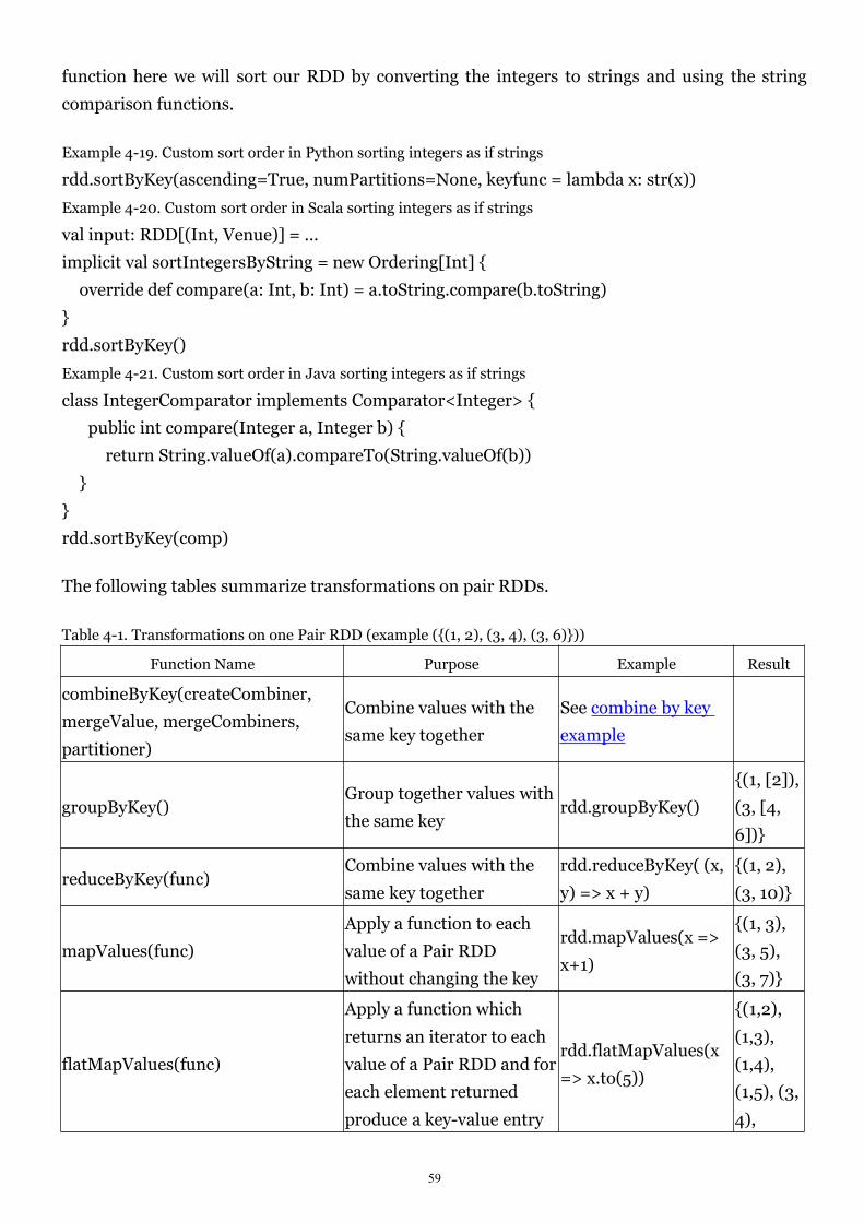
59
function here we will sort our RDD by converting the integers to strings and using the string
comparison functions.
Example 4-19. Custom sort order in Python sorting integers as if strings
rdd.sortByKey(ascending=True, numPartitions=None, keyfunc = lambda x: str(x))
Example 4-20. Custom sort order in Scala sorting integers as if strings
val input: RDD[(Int, Venue)] = ...
implicit val sortIntegersByString = new Ordering[Int] {
override def compare(a: Int, b: Int) = a.toString.compare(b.toString)
}
rdd.sortByKey()
Example 4-21. Custom sort order in Java sorting integers as if strings
class IntegerComparator implements Comparator<Integer> {
public int compare(Integer a, Integer b) {
return String.valueOf(a).compareTo(String.valueOf(b))
}
}
rdd.sortByKey(comp)
The following tables summarize transformations on pair RDDs.
Table 4-1. Transformations on one Pair RDD (example ({(1, 2), (3, 4), (3, 6)}))
Function Name Purpose Example Result
combineByKey(createCombiner,
mergeValue, mergeCombiners,
partitioner)
Combine values with the
same key together
See combine by key
example
groupByKey()Group together values with
the same keyrdd.groupByKey()
{(1, [2]),
(3, [4,
6])}
reduceByKey(func)Combine values with the
same key together
rdd.reduceByKey( (x,
y) => x + y)
{(1, 2),
(3, 10)}
mapValues(func)
Apply a function to each
value of a Pair RDD
without changing the key
rdd.mapValues(x =>
x+1)
{(1, 3),
(3, 5),
(3, 7)}
flatMapValues(func)
Apply a function which
returns an iterator to each
value of a Pair RDD and for
each element returned
produce a key-value entry
rdd.flatMapValues(x
=> x.to(5))
{(1,2),
(1,3),
(1,4),
(1,5), (3,
4),
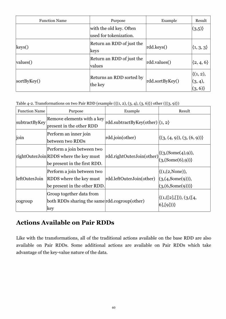
60
Function Name Purpose Example Result
with the old key. Often
used for tokenization.
(3,5)}
keys()Return an RDD of just the
keysrdd.keys() {1, 3, 3}
values()Return an RDD of just the
valuesrdd.values() {2, 4, 6}
sortByKey()Returns an RDD sorted by
the keyrdd.sortByKey()
{(1, 2),
(3, 4),
(3, 6)}
Table 4-2. Transformations on two Pair RDD (example ({(1, 2), (3, 4), (3, 6)}) other ({(3, 9)})
Function Name Purpose Example Result
subtractByKeyRemove elements with a key
present in the other RDDrdd.subtractByKey(other) {1, 2}
joinPerform an inner join
between two RDDsrdd.join(other) {(3, (4, 9)), (3, (6, 9))}
rightOuterJoin
Perform a join between two
RDDS where the key must
be present in the first RDD.
rdd.rightOuterJoin(other){(3,(Some(4),9)),
(3,(Some(6),9))}
leftOuterJoin
Perform a join between two
RDDS where the key must
be present in the other RDD.
rdd.leftOuterJoin(other)
{(1,(2,None)),
(3,(4,Some(9))),
(3,(6,Some(9)))}
cogroup
Group together data from
both RDDs sharing the same
key
rdd.cogroup(other){(1,([2],[])), (3,([4,
6],[9]))}
Actions Available on Pair RDDs
Like with the transformations, all of the traditional actions available on the base RDD are also
available on Pair RDDs. Some additional actions are available on Pair RDDs which take
advantage of the key-value nature of the data.
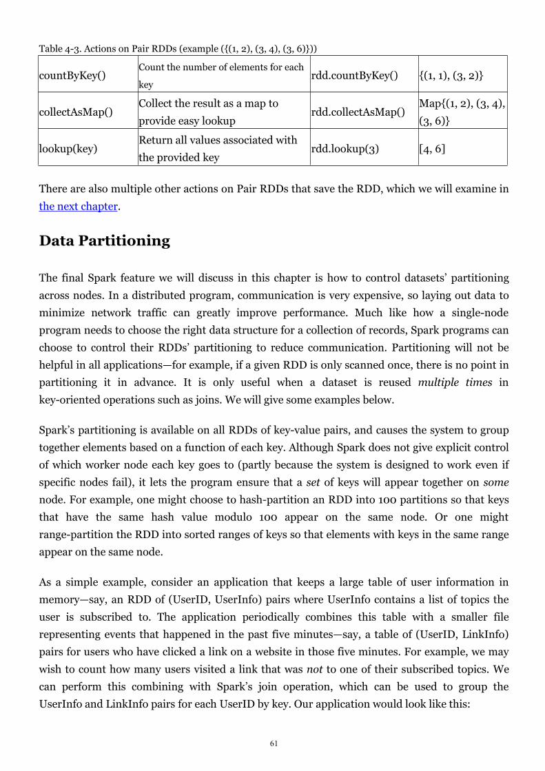
61
Table 4-3. Actions on Pair RDDs (example ({(1, 2), (3, 4), (3, 6)}))
countByKey()Count the number of elements for each
keyrdd.countByKey() {(1, 1), (3, 2)}
collectAsMap()Collect the result as a map to
provide easy lookuprdd.collectAsMap()
Map{(1, 2), (3, 4),
(3, 6)}
lookup(key)Return all values associated with
the provided keyrdd.lookup(3) [4, 6]
There are also multiple other actions on Pair RDDs that save the RDD, which we will examine in
the next chapter.
Data Partitioning
The final Spark feature we will discuss in this chapter is how to control datasets’ partitioning
across nodes. In a distributed program, communication is very expensive, so laying out data to
minimize network traffic can greatly improve performance. Much like how a single-node
program needs to choose the right data structure for a collection of records, Spark programs can
choose to control their RDDs’ partitioning to reduce communication. Partitioning will not be
helpful in all applications—for example, if a given RDD is only scanned once, there is no point in
partitioning it in advance. It is only useful when a dataset is reused multiple times in
key-oriented operations such as joins. We will give some examples below.
Spark’s partitioning is available on all RDDs of key-value pairs, and causes the system to group
together elements based on a function of each key. Although Spark does not give explicit control
of which worker node each key goes to (partly because the system is designed to work even if
specific nodes fail), it lets the program ensure that a set of keys will appear together on some
node. For example, one might choose to hash-partition an RDD into 100 partitions so that keys
that have the same hash value modulo 100 appear on the same node. Or one might
range-partition the RDD into sorted ranges of keys so that elements with keys in the same range
appear on the same node.
As a simple example, consider an application that keeps a large table of user information in
memory—say, an RDD of (UserID, UserInfo) pairs where UserInfo contains a list of topics the
user is subscribed to. The application periodically combines this table with a smaller file
representing events that happened in the past five minutes—say, a table of (UserID, LinkInfo)
pairs for users who have clicked a link on a website in those five minutes. For example, we may
wish to count how many users visited a link that was not to one of their subscribed topics. We
can perform this combining with Spark’s join operation, which can be used to group the
UserInfo and LinkInfo pairs for each UserID by key. Our application would look like this:
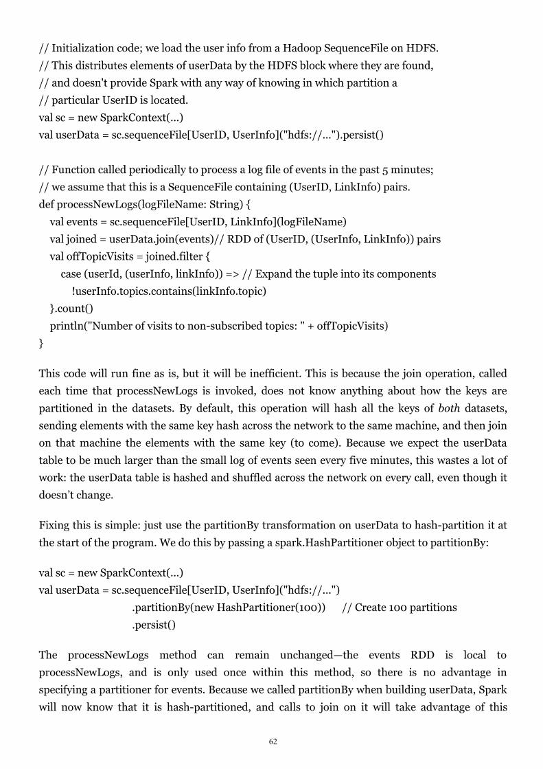
62
// Initialization code; we load the user info from a Hadoop SequenceFile on HDFS.
// This distributes elements of userData by the HDFS block where they are found,
// and doesn't provide Spark with any way of knowing in which partition a
// particular UserID is located.
val sc = new SparkContext(...)
val userData = sc.sequenceFile[UserID, UserInfo]("hdfs://...").persist()
// Function called periodically to process a log file of events in the past 5 minutes;
// we assume that this is a SequenceFile containing (UserID, LinkInfo) pairs.
def processNewLogs(logFileName: String) {
val events = sc.sequenceFile[UserID, LinkInfo](logFileName)
val joined = userData.join(events)// RDD of (UserID, (UserInfo, LinkInfo)) pairs
val offTopicVisits = joined.filter {
case (userId, (userInfo, linkInfo)) => // Expand the tuple into its components
!userInfo.topics.contains(linkInfo.topic)
}.count()
println("Number of visits to non-subscribed topics: " + offTopicVisits)
}
This code will run fine as is, but it will be inefficient. This is because the join operation, called
each time that processNewLogs is invoked, does not know anything about how the keys are
partitioned in the datasets. By default, this operation will hash all the keys of both datasets,
sending elements with the same key hash across the network to the same machine, and then join
on that machine the elements with the same key (to come). Because we expect the userData
table to be much larger than the small log of events seen every five minutes, this wastes a lot of
work: the userData table is hashed and shuffled across the network on every call, even though it
doesn’t change.
Fixing this is simple: just use the partitionBy transformation on userData to hash-partition it at
the start of the program. We do this by passing a spark.HashPartitioner object to partitionBy:
val sc = new SparkContext(...)
val userData = sc.sequenceFile[UserID, UserInfo]("hdfs://...")
.partitionBy(new HashPartitioner(100)) // Create 100 partitions
.persist()
The processNewLogs method can remain unchanged—the events RDD is local to
processNewLogs, and is only used once within this method, so there is no advantage in
specifying a partitioner for events. Because we called partitionBy when building userData, Spark
will now know that it is hash-partitioned, and calls to join on it will take advantage of this
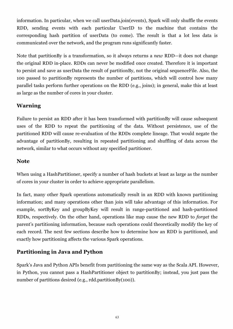
63
information. In particular, when we call userData.join(events), Spark will only shuffle the events
RDD, sending events with each particular UserID to the machine that contains the
corresponding hash partition of userData (to come). The result is that a lot less data is
communicated over the network, and the program runs significantly faster.
Note that partitionBy is a transformation, so it always returns a new RDD—it does not change
the original RDD in-place. RDDs can never be modified once created. Therefore it is important
to persist and save as userData the result of partitionBy, not the original sequenceFile. Also, the
100 passed to partitionBy represents the number of partitions, which will control how many
parallel tasks perform further operations on the RDD (e.g., joins); in general, make this at least
as large as the number of cores in your cluster.
Warning
Failure to persist an RDD after it has been transformed with partitionBy will cause subsequent
uses of the RDD to repeat the partitioning of the data. Without persistence, use of the
partitioned RDD will cause re-evaluation of the RDDs complete lineage. That would negate the
advantage of partitionBy, resulting in repeated partitioning and shuffling of data across the
network, similar to what occurs without any specified partitioner.
Note
When using a HashPartitioner, specify a number of hash buckets at least as large as the number
of cores in your cluster in order to achieve appropriate parallelism.
In fact, many other Spark operations automatically result in an RDD with known partitioning
information; and many operations other than join will take advantage of this information. For
example, sortByKey and groupByKey will result in range-partitioned and hash-partitioned
RDDs, respectively. On the other hand, operations like map cause the new RDD to forget the
parent’s partitioning information, because such operations could theoretically modify the key of
each record. The next few sections describe how to determine how an RDD is partitioned, and
exactly how partitioning affects the various Spark operations.
Partitioning in Java and Python
Spark’s Java and Python APIs benefit from partitioning the same way as the Scala API. However,
in Python, you cannot pass a HashPartitioner object to partitionBy; instead, you just pass the
number of partitions desired (e.g., rdd.partitionBy(100)).

64
Determining an RDD’s Partitioner
In Scala and Java, you can determine how an RDD is partitioned using its partitioner property
(or partitioner() method in Java).[9] This returns a scala.Option object, which is a Scala class for
a container that may or may not contain one item. (It is considered good practice in Scala to use
Option for fields that may not be present, instead of setting a field to null if a value is not present,
running the risk of a null-pointer exception if the program subsequently tries to use the null as if
it were an actual, present value.) You can call isDefined() on the Option to check whether it has a
value, and get() to get this value. If present, the value will be a spark.Partitioner object. This is
essentially a function telling the RDD which partition each key goes into—more about this later.
The partitioner property is a great way to test in the Spark shell how different Spark operations
affect partitioning, and to check that the operations you want to do in your program will yield
the right result. For example:
scala> val pairs = sc.parallelize(List((1, 1), (2, 2), (3, 3)))
pairs: spark.RDD[(Int, Int)] = ParallelCollectionRDD[0] at parallelize at <console>:12
scala> pairs.partitioner
res0: Option[spark.Partitioner] = None
scala> val partitioned = pairs.partitionBy(new spark.HashPartitioner(2))
partitioned: spark.RDD[(Int, Int)] = ShuffledRDD[1] at partitionBy at <console>:14
scala> partitioned.partitioner
res1: Option[spark.Partitioner] = Some(spark.HashPartitioner@5147788d)
In this short session, we created an RDD of (Int, Int) pairs, which initially have no partitioning
information (an Option with value None). We then created a second RDD by hash-partitioning
the first. If we actually wanted to use partitioned in further operations, then we should have
appended .cache() to the third line of input, in which partitioned is defined. This is for the same
reason that we needed cache for userData in the previous example: without cache, subsequent
RDD actions will evaluate the entire lineage of partitioned, which will cause pairs to be
hash-partitioned over and over.
Operations that Benefit from Partitioning
Many of Spark’s operations involve shuffling data by key across the network. All of these will
benefit from partitioning. As of Spark 1.0, the operations that benefit from partitioning are:
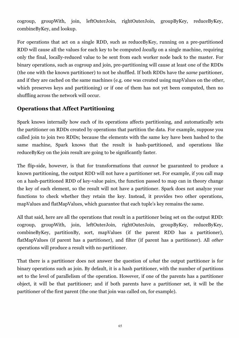
65
cogroup, groupWith, join, leftOuterJoin, rightOuterJoin, groupByKey, reduceByKey,
combineByKey, and lookup.
For operations that act on a single RDD, such as reduceByKey, running on a pre-partitioned
RDD will cause all the values for each key to be computed locally on a single machine, requiring
only the final, locally-reduced value to be sent from each worker node back to the master. For
binary operations, such as cogroup and join, pre-partitioning will cause at least one of the RDDs
(the one with the known partitioner) to not be shuffled. If both RDDs have the same partitioner,
and if they are cached on the same machines (e.g. one was created using mapValues on the other,
which preserves keys and partitioning) or if one of them has not yet been computed, then no
shuffling across the network will occur.
Operations that Affect Partitioning
Spark knows internally how each of its operations affects partitioning, and automatically sets
the partitioner on RDDs created by operations that partition the data. For example, suppose you
called join to join two RDDs; because the elements with the same key have been hashed to the
same machine, Spark knows that the result is hash-partitioned, and operations like
reduceByKey on the join result are going to be significantly faster.
The flip-side, however, is that for transformations that cannot be guaranteed to produce a
known partitioning, the output RDD will not have a partitioner set. For example, if you call map
on a hash-partitioned RDD of key-value pairs, the function passed to map can in theory change
the key of each element, so the result will not have a partitioner. Spark does not analyze your
functions to check whether they retain the key. Instead, it provides two other operations,
mapValues and flatMapValues, which guarantee that each tuple’s key remains the same.
All that said, here are all the operations that result in a partitioner being set on the output RDD:
cogroup, groupWith, join, leftOuterJoin, rightOuterJoin, groupByKey, reduceByKey,
combineByKey, partitionBy, sort, mapValues (if the parent RDD has a partitioner),
flatMapValues (if parent has a partitioner), and filter (if parent has a partitioner). All other
operations will produce a result with no partitioner.
That there is a partitioner does not answer the question of what the output partitioner is for
binary operations such as join. By default, it is a hash partitioner, with the number of partitions
set to the level of parallelism of the operation. However, if one of the parents has a partitioner
object, it will be that partitioner; and if both parents have a partitioner set, it will be the
partitioner of the first parent (the one that join was called on, for example).
66
Example: PageRank
As an example of a more involved algorithm that can benefit from RDD partitioning, we
consider PageRank. The PageRank algorithm, named after Google’s Larry Page, aims to assign a
measure of importance (a “rank”) to each document in a set based on how many documents
have links to it. It can be used to rank web pages, of course, but also scientific articles, or
influential users in a social network (by treating each user as a “document” and each friend
relationship as a “link”).
PageRank is an iterative algorithm that performs many joins, so it is a good use case for RDD
partitioning. The algorithm maintains two datasets: one of (pageID, linkList) elements
containing the list of neighbors of each page, and one of (pageID, rank) elements containing the
current rank for each page. It proceeds as follows:
1. Initialize each page’s rank to 1.0
2. On each iteration, have page p send a contribution of rank(p) / numNeighbors(p) to its neighbors
(the pages it has links to).
3. Set each page’s rank to 0.15 + 0.85 * contributionsReceived.
The last two steps repeat for several iterations, during which the algorithm will converge to the
correct PageRank value for each page. As a simple solution, it’s typically enough to run about ten
iterations and declare the resulting ranks to be the PageRank values.
Here is the code to implement PageRank in Spark:
val sc = new SparkContext(...)
// Assume that our neighbor list was saved as a Spark objectFile
val links = sc.objectFile[(String, Seq[String])]("links")
.partitionBy(new HashPartitioner(100))
.persist()
// Initialize each page's rank to 1.0; since we use mapValues, the resulting RDD
// will have the same partitioner as links
var ranks = links.mapValues(_ => 1.0)
// Run 10 iterations of PageRank
for (i <- 0 until 10) {
val contributions = links.join(ranks).flatMap {
case (pageId, (links, rank)) =>
67
links.map(dest => (dest, rank / links.size))
}
ranks = contributions.reduceByKey(_ + _).mapValues(0.15 + 0.85 * _)
}
// Write out the final ranks
ranks.saveAsTextFile("ranks")
That’s it! The algorithm starts with a ranks RDD initialized at 1.0 for each element, and keeps
updating the ranks variable on each iteration. The body of PageRank is pretty simple to express
in Spark: it first does a join between the current ranks RDD and the static links one, in order to
obtain the link list and rank for each page ID together, then uses this in a flatMap to create
“contribution” values to send to each of the page’s neighbors. We then add up these values by
page ID (i.e. by the page receiving the contribution) and set that page’s rank to 0.15 + 0.85 *
contributionsReceived.
Although the code itself is simple, the example does several things to ensure that the RDDs are
partitioned in an efficient way, and to minimize communication:
1. Notice that the links RDD is joined against ranks on each iteration. Since links is a static dataset, we
partition it at the start with partitionBy, so that it does not need to be shuffled across the network. In
practice, the links RDD is also likely to be much larger in terms of bytes than ranks, since it contains
a list of neighbors for each page ID instead of just a Double, so this optimization saves considerable
network traffic over a simple implementation of PageRank (e.g. in plain MapReduce).
2. For the same reason, we call persist on links to keep it in RAM across iterations.
3. When we first create ranks, we use mapValues instead of map to preserve the partitioning of the
parent RDD (links), so that our first join against it is very cheap.
4. In the loop body, we follow our reduceByKey withmapValues; because the result of reduceByKey
is already hash-partitioned, this will make it more efficient to join the mapped result against links on
the next iteration.
Finally, note also that the extra syntax from using partitioning is small, and mapValues in
particular is more concise in the places it’s used here than a map.
Note
To maximize the potential for partitioning-related optimizations, you should use mapValues or
flatMapValues whenever you are not changing an element’s key.

68
Custom Partitioners
While Spark’s HashPartitioner and RangePartitioner are well-suited to many use cases, Spark
also allows you to tune how an RDD is partitioned by providing a custom Partitioner object. This
can be used to further reduce communication by taking advantage of domain-specific
knowledge.
For example, suppose we wanted to run the PageRank algorithm in the previous section on a set
of web pages. Here each page’s ID (the key in our RDD) will be its URL. Using a simple hash
function to do the partitioning, pages with similar URLs (e.g., http://www.cnn.com/WORLD
and http://www.cnn.com/US) might be hashed to completely different nodes. However, we
know that web pages within the same domain tend to link to each other a lot. Because PageRank
needs to send a message from each page to each of its neighbors on each iteration, it helps to
group these pages into the same partition. We can do this with a custom Partitioner that looks at
just the domain name instead of the whole URL.
To implement a custom partitioner, you need to subclass the spark.Partitioner class and
implement three methods:
numPartitions: Int, which returns the number of partitions you will create
getPartition(key: Any): Int, which returns the partition ID (0 to numPartitions-1) for a given key
equals, the standard Java equality method. This is important to implement because Spark will need
to test your Partitioner object against other instances of itself when it decides whether two of your
RDDs are partitioned in the same way!
One gotcha is that, if you rely on Java’s hashCode method in your algorithm, it can return
negative numbers. You need to be careful that getPartition always returns a non-negative result.
For example, here is how we would write the domain-name based partitioner sketched above,
which hashes only the domain name of each URL:
class DomainNamePartitioner(numParts: Int) extends Partitioner {
override def numPartitions: Int = numParts
override def getPartition(key: Any): Int = {
val domain = new java.net.URL(key.toString).getHost()
val code = (domain.hashCode % numPartitions)
if (code < 0) {
code + numPartitions // Make it non-negative
} else {
69
code
}
}
// Java equals method to let Spark compare our Partitioner objects
override def equals(other: Any): Boolean = other match {
case dnp: DomainNamePartitioner =>
dnp.numPartitions == numPartitions
case _ =>
false
}
}
Note that in the equals method, we used Scala’s pattern matching operator (match) to test
whether other is a DomainNamePartitioner, and cast it if so; this is the same as using instanceof
in Java.
Using a custom Partitioner is easy: just pass it to the partitionBy method. Many of the
shuffle-based methods in Spark, such as join and groupByKey, can also take an optional
Partitioner object to +control the partitioning of the output.
Creating a custom Partitioner in Java is very similar to Scala: just extend the spark.Partitioner
class and implement the required methods.
In Python, you do not extend a Partitioner class, but instead pass a hash function as an
additional argument to RDD.partitionBy(). For example:
import urlparse
def hash_domain(url):
return hash(urlparse.urlparse(url).netloc)
rdd.partitionBy(20, hash_domain) # Create 20 partitions
Note that the hash function you pass will be compared by identity to that of other RDDs. If you
want to partition multiple RDDs with the same partitioner, pass the same function object (e.g., a
global function) instead of creating a new lambda for each one!
70
Conclusion
In this chapter, we have seen how to work with keyed data using the specialized functions
available in Spark. The techniques from the previous chapter on Programming with RDDs also
still work on our Pair RDDs. In the next chapter, we will look at how to load and save data.
[9] The Python API does not yet offer a way to query partitioners, though it still uses them
internally.

71
Chapter 5. Loading and Saving Your Data
Both engineers and data scientists will find parts of this chapter useful. Engineers may wish to
explore more output formats to see if there is something well suited to their intended down
stream consumer available and should consider looking online for different Hadoop formats.
Data Scientists can likely focus on the input format that their data is already in. Spark supports
reading from classes that implement Hadoop’s InputFormat and writing to Hadoop’s
OutputFormat interfaces.
Motivation
We’ve looked at a number of operations we can perform on our data once we have it distributed
in Spark. So far our examples have loaded and saved all of their data from a native collection
and regular files, but odds are that your data doesn’t fit on a single machine, so its time to
explore our options.
In addition to different formats, we also have different compression options which can decrease
the amount of space and network overhead required but can introduce restrictions on how we
read the data. There are myriad of different data sources and formats we can use to create a new
RDD and we will only cover the most common here.
Note
In Spark 1.0, the standard data APIs for Python only support text data. However, you can work
around this by using Spark SQL, which allows loading data from a number of formats supported
by Hive. We will cover Spark SQL in a later chapter, but briefly illustrate how to load data from
Hive in this chapter too.
Choosing a Format
Often when we need data for our code we don’t get to choose the format. Sometimes we are
lucky enough to be able to choose from multiple formats or work with our upstream data
providers. We will start with some common file formats which we can write to a number of
different file systems. In addition to standard file formats, we will also examine using different
database systems for IO. Spark works with all the formats implementing Hadoop’s InputFormat
and OutputFormat interfaces.

72
Table 5-1. Common Supported File Formats
Format
nameSplittable Structured comments
text files yes noPlain old text files. Splittable provided
records are one per line.
JSON yes semi
Common text based format, are
semi-structured, splittable if one record per
line.
CSV yes yesVery common text based format, often used
with spreadsheet applications.
Sequence
filesyes yes
A common Hadoop file format used for
key-value data.
Protocol
Buffersyes yes A fast space-efficient multi-language format.
Object
Filesyes yes
Useful for saving data from a Spark job to be
consumed by shared code. Breaks if you
change your classes, as it relies on Java
Serialization.
In addition to these file formats, Spark can also work directly with a number of database and
search systems. We will look at Mongo, Hive, Cassandra, and Elasticsearch, but many more are
supported through the standard Hadoop connectors with Spark. This is convenient if your data
happens to already be in one of these systems as nightly dumps of data can be difficult to
maintain. When about to run a new Spark job against an on-line system you should verify you
have sufficient capacity for a potentially very high volume of queries.
Formats
Spark makes it very simple to load and save data in a large number of formats. Formats range
from unstructured, like text, to semi-structured, like JSON, and to structured like Sequence
Files. The input formats that Spark wraps all transparently handle compressed formats based on
the file extension.
In addition to the output mechanism supported directly in Spark, we can use both Hadoop’s
new and old file APIs for keyed (or paired) data. This restriction exists because the Hadoop
interfaces require key-value data, although some formats ignore the key.
73
Text Files
Text files are very simple to load from and save to with Spark. When we load a single text file as
an RDD each input line becomes an element in the RDD. We can also load multiple whole text
files at the same time into a Pair RDD with the key being the name and the value being the
contents of each file.
Loading a single text file is as simple as calling the textFile function on our spark context with
the path to the file. If we want to control the number of partitions that the we can also specify
minPartitions.
Example 5-1. Python load text file example
input = sc.textFile("file:///home/holden/repos/spark/README.md")
Example 5-2. Scala load text file example
val input = sc.textFile("file:///home/holden/repos/spark/README.md")
Example 5-3. Java load text file example
JavaRDD<String> input = sc.textFile("file:///home/holden/repos/spark/README.md")
Multi-part inputs in the form of a directory containing all of the parts can be handled in two
ways. We can just use same textFile method and pass it a directory and it will load all of the
parts into our RDD. Sometimes its important to know which file which piece of input came from
(such as time data with the key in the file) or we need to process an entire file at a time. If our
files are small enough then we can use the wholeTextFiles method and get back a Pair RDD
where the key is the name of the input file.
wholeTextFiles can be very useful when each file represents a certain time periods data. If we
had files representing sales data from different periods we could easily compute the average for
each period.
Example 5-4. Scala average value per file
val input = sc.wholeTextFiles("file://home/holden/happypanda")
val result = input.mapValues{y =>
val nums = y.split(" ").map(x => x.toDouble)
nums.sum / nums.size.toDouble
}
Tip
Spark supports reading all the files in a given directory and doing wild card expansion on the
input (e.g. part-*.txt). This is useful since large data sets are often spread across multiple files.
74
Outputting text files is also quite simple. The method saveAsTextFile takes a path and will
output the contents of the RDD to that file. The path is treated as a directory and Spark will
output multiple files underneath that directory. This allows Spark to write the output from
multiple nodes. With this method we don’t get to control which files end up with which
segments of our data but there are other output formats which do allow this.
Example 5-5. Scala save as text file example
result.saveAsTextFile(outputFile)
Loading and saving text files is implemented through wrappers around Hadoop’s file APIs. If
you want further examples of how to work with the Hadoop file APIs you can see how this is
implemented in SparkContext and RDD respectively.
JSON
JSON is a popular semi-structured data format. The simplest way to load JSON data is by
loading the data as a text file and then mapping over the values with a JSON parser. Like wise,
we can use our preferred JSON serialization library to write out the values to strings which we
can then write out. In Java and Scala we can also work with JSON data using a custom Hadoop
format.
Loading the data as a text file and then parsing the JSON data is an approach that we can use in
all of the supported languages. This works assuming that you have one JSON record per-row, if
you have multi-line JSON files you will instead have to load the whole file and then parse each
file. If constructing a JSON parser is expensive in your language, you can use mapPartitions to
re-use the parser.
There are a wide variety of JSON libraries available for the three languages we are looking at, for
simplicities sake we are only considering one library per language. In Java we will use Jackson,
in Scala we are using liftweb-json, and in python we use the built in library. These libraries have
been chosen as they perform reasonable well and are also relatively simple, if you spend a lot of
time in the parsing stage you may wish to look at other JSON libraries for Scala or for Java.
Example 5-6. Python load JSON example
data = input.map(lambda x: json.loads(x))
Example 5-7. Scala load JSON example
import play.api.libs.json._
import play.api.libs.functional.syntax._
...
val parsed = input.map(Json.parse(_))
75
If your JSON data happens to follow a predictable schema (lucky you!), we can parse it into a
more structured format. This is often where we will find invalid records, so we may wish to skip
them.
Example 5-8. Scala load JSON example
case class Person(name: String, lovesPandas: Boolean)
implicit val personReads = Json.format[Person]
// We use asOpt combined with flatMap so that if it fails to parse we
// get back a None and the flatMap essentially skips the result.
val parsed = input.flatMap(record =>
personReads.read(JSON.parseFull(record)).asOpt)
Example 5-9. Java load JSON example
public static class ParseJson implements FlatMapFunction<Iterator<String>, Person> {
public Iterable<Person> call(Iterator<String> lines) throws Exception {
ArrayList<Person> people = new ArrayList<Person>();
ObjectMapper mapper = new ObjectMapper();
while (lines.hasNext()) {
String line = lines.next();
try {
people.add(mapper.readValue(line, Person.class));
} catch (Exception e) {
// skip records on failure
}
}
return people;
}
}
Tip
Handling incorrectly formatted records can be a big problem, especially with semi-structured
data like JSON. With small data sets it can be acceptable to stop the world (i.e. fail the program)
on malformed input, but often with large data sets malformed input is simply a part of life. If
you do choose to skip incorrectly formatted (or attempt to recover) incorrectly formatted data
you may wish to look at using accumulators to keep track of the number of errors.
Writing out JSON files is much simpler compared to loading it as we don’t have to worry about
incorrectly formatted data and we know the type of the data that we are writing out. We can use
the same librariess we used to convert our RDD of strings into parsed JSON data and instead

76
take our RDD of structured data and convert it into an RDD of strings which we can then write
out using Spark’s text file API.
Lets say we were running a promotion for people that love pandas, so we can take our input
from the first step and filter it for the people that love pandas.
Example 5-10. Python save JSON example
(data.filter(lambda x: x['lovesPandas']).map(lambda x: json.dumps(x))
.saveAsTextFile(outputFile))
Example 5-11. Scala save JSON example
result.filter(x => x.lovesPandas).map(x => Json.toJson(x)).
saveAsTextFile(outputFile)
Example 5-12. Java save JSON example
public static class WriteJson implements
FlatMapFunction<Iterator<Person>, String> {
public Iterable<String> call(Iterator<Person> people) throws Exception {
ArrayList<String> text = new ArrayList<String>();
ObjectMapper mapper = new ObjectMapper();
while (people.hasNext()) {
Person person = people.next();
text.add(mapper.writeValueAsString(person));
}
return text;
}
}
JavaRDD<Person> result = input.mapPartitions(new ParseJson()).filter(
new LikesPandas());
JavaRDD<String> formatted = result.mapPartitions(new WriteJson());
formatted.saveAsTextFile(outfile);
We can easily load and save JSON data with Spark by using the existing mechanism for working
with text and adding JSON libraries.
CSV (Comma Separated Values) / TSV (Tab Separated Values)
CSV files are supposed to contain a fixed number of fields per-line, and the fields are most
commonly separated by comma or tab. Records are often stored one per line, but this is not
always the case as records can sometimes span lines. CSV/TSV files can sometimes be
inconsistent, most frequently in respect to handling newlines, escaping, non-ASCII characters,
77
non-integer numbers. CSVs cannot handle nested field types natively, so we have to unpack and
pack to specific fields manually.
Unlike with JSON fields each record doesn’t have field names associated with them; instead we
get back row numbers. It is common practice in single CSV files to have the first rows column
values be the names of each field.
Loading CSV/TSV data is similar to loading JSON data in that we can first load it as text and
then process it. The lack of standardization leads to different versions of the same library
sometimes handling input in different ways.
Like with JSON there are many different CSV libraries and we will only use one for each
language. In both Scala and Java we use opencsv. Once again in Python we use the included csv
library.
Tip
As with JSON there is a Hadoop CSVInputFormat that we can use to load CSV data in Scala and
Java (although it does not support records containing newlines).
If your CSV data happens to not contain newlines in any of the fields, you can load your data
with textFile and parse it.
Example 5-13. Python load CSV example
import csv
import StringIO
...
def loadRecord(line):
"""Parse a CSV line"""
input = StringIO.StringIO(line)
reader = csv.DictReader(input, fieldnames=["name", "favouriteAnimal"])
return reader.next()
input = sc.textFile(inputFile).map(loadRecord)
Example 5-14. Java load CSV example
import au.com.bytecode.opencsv.CSVReader;
...
public static class ParseLine implements Function<String, String[]> {
public String[] call(String line) throws Exception {
CSVReader reader = new CSVReader(new StringReader(line));
return reader.readNext();
78
}
}
JavaRDD<String> csvFile1 = sc.textFile(csv1);
JavaPairRDD<String[]> csvData = csvFile1.map(new ParseLine());
Example 5-15. Scala load CSV example
import au.com.bytecode.opencsv.CSVReader
...
val input = sc.textFile(inputFile)
val result = input.map{ line =>
val reader = new CSVReader(new StringReader(line));
reader.readNext();
}
If there are embedded newlines in fields we will need to load each file in full and parse the entire
segment. This is unfortunate as if each file is large this can easily introduce bottlenecks in
loading and parsing.
Example 5-16. Python load CSV example
def loadRecords(fileNameContents):
"""Load all the records in a given file"""
input = StringIO.StringIO(fileNameContents[1])
reader = csv.DictReader(input, fieldnames=["name", "favoriteAnimal"])
return reader
fullFileData = sc.wholeTextFiles(inputFile).flatMap(loadRecords)
Example 5-17. Java load CSV example
public static class ParseLine implements FlatMapFunction<Tuple2<String, String>, String[]> {
public Iterable<String[]> call(Tuple2<String, String> file) throws Exception {
CSVReader reader = new CSVReader(new StringReader(file._2()));
return reader.readAll();
}
}
JavaPairRDD<String, String> csvData = sc.wholeTextFiles(csvInput);
JavaRDD<String[]> keyedRDD = csvData.flatMap(new ParseLine());
Example 5-18. Scala load CSV example
case class Person(name: String, favoriteAnimal: String)
val input = sc.wholeTextFiles(inputFile)
val result = input.flatMap{ case (_, txt) =>
val reader = new CSVReader(new StringReader(txt));

79
reader.readAll().map(x => Person(x(0), x(1)))
}
Tip
If there are only a few input files you may want to repartition your input to allow Spark to
effectively parallelize your future operations.
As with JSON data, writing out CSV/TSV data is quite simple and we can benefit from reusing
the output encoding object. Since in CSV we don’t output the field name with each record, to
have a consistent output we need to create a mapping. One of the easy ways to do this is to just
write a function which converts the fields to given positions in an array. In Python if we are
outputting dictionaries the csv writer can do this for us based on the order we provide the
feildnames when constructing the writer.
The CSV libraries we are using output to files/writers so we can use StringWriter/StringIO to
allow us to put the result in our RDD.
Example 5-19. Python write csv example
def writeRecords(records):
"""Write out CSV lines"""
output = StringIO.StringIO()
writer = csv.DictWriter(output, fieldnames=["name", "favoriteAnimal"])
for record in records:
writer.writerow(record)
return [output.getvalue()]
pandaLovers.mapPartitions(writeRecords).saveAsTextFile(outputFile)
Example 5-20. Scala write CSV example
pandaLovers.map(person => List(person.name, person.favoriteAnimal).toArray)
.mapPartitions{people =>
val stringWriter = new StringWriter();
val csvWriter = new CSVWriter(stringWriter);
csvWriter.writeAll(people.toList)
Iterator(stringWriter.toString)
}.saveAsTextFile(outFile)
As you may have noticed the above only works provided that we know all of the fields that we
will be outputting. However, if some of the field names are determined at runtime from user

80
input we need to take a different approach. The simplest approach is going over all of our data
and extracting the distinct keys.
Sequence Files
Sequence files are a popular Hadoop format comprised of flat files with key-value pairs and are
supported in Spark’s Java and Scala APIs. Sequence files have sync markers that allow Spark to
seek to a point in the file and then resychronize with the record boundaries. This allows Spark to
efficiently read Sequence files in from multiple nodes and in to many partitions. Sequence Files
are a common input/output format for Hadoop MapReduce jobs as well so if you are working
with an existing Hadoop system there is a good change your data will be available as a sequence
file.
Sequence files consist of elements which implement Hadoop’s Writable interface, as Hadoop
uses a custom serialization framework. We have a conversion table of some common types and
their corresponding Writable class. The standard rule of thumb is try adding the word Writable
to the end of your class name and see if it is a known subclass of org.apache.hadoop.io.Writable.
If you can’t find a Writable for the data you are trying to write out (like for example a custom
case class), you can go ahead and implement your own Writable class by overriding readFields
and write from org.apache.hadoop.io.Writable.
Warning
Hadoop’s RecordReader re-uses the same object for each record, so directly calling cache, on an
RDD you read in like this can fail, instead add a simple map operation and cache the result of
the map. Further more, many Hadoop Writable classes do not implement java.io.Serializable so
for them to work in RDDs we need to convert them with a map anyways.
Table 5-2. Corresponding Hadoop Writable Types
Scala Type Java Type Hadoop Writable
Int Integer IntWritable or VIntWritable [a]
Long Long LongWritable or VLongWritable [a]
Float Float FloatWritable
Double Double DoubleWritable
Boolean Boolean BooleanWritable
Array[Byte] Byte[] BytesWritable
String String Text
Array[T] T[] ArrayWritable<TW> [b]
List[T] List<T> ArrayWritable<TW> [b]

81
Scala Type Java Type Hadoop Writable
Map[A, B] Map<A, B> MapWritable<AW, BW> [b]
[a] ints and longs are often stored as a fixed size. Storing the number 12 takes the same amount of
space as storing the number 2**30. If you might have a large number of small numbers. Instead
we can use variable sized types which will use less bits to store smaller numbers.
[b]The templated type must also be a writable type.
Spark has a specialized API for reading in sequence files. On the Spark Context we can call
sequenceFile(path, keyClass, valueClass, minPartitions). As mentioned earlier, Sequence Files
work with Writable classes, so our keyClass and valueClass will both have to be the correct
Writable class. Lets consider loading people and the number of pandas they have seen from a
sequence file, in this case our keyClass would be Text and our valueClass would be IntWritable
or VIntWritable, for simplicity lets work with IntWritable.
Example 5-21. Scala load sequence file example
val data = sc.sequenceFile(inFile, classOf[Text], classOf[IntWritable]).
map{case (x, y) => (x.toString, y.get())}
Example 5-22. Java load sequence file example
public static class ConvertToNativeTypes implements
PairFunction<Tuple2<Text, IntWritable>, String, Integer> {
public Tuple2<String, Integer> call(Tuple2<Text, IntWritable> record) {
return new Tuple2(record._1.toString(), record._2.get());
}
}
JavaPairRDD<Text, IntWritable> input = sc.sequenceFile(fileName, Text.class,
IntWritable.class);
JavaPairRDD<String, Integer> result = input.mapToPair(
new ConvertToNativeTypes());
Tip
In Scala there is a convenience function which can automatically convert Writables to their
corresponding Scala type. Instead of specifying the keyClass and valueClass we can call
sequenceFile[Key, Class](path, minPartitions) and get back an RDD of native Scala types.
Writing the data out to a sequence file is fairly similar in Scala. First since sequence files are
key-value pairs, we need a PairRDD with types that our sequence file can write out. Implicit
conversions between Scala types and Hadoop Writables exist for many native types, so if you are
82
writing out a native type you can just save your PairRDD by calling saveAsSequenceFile(path)
and it will write out the data for us. If there isn’t an automatic conversion from our key and
value to Writable, or we want to use VarInts we can just map over the data and convert it before
saving. Lets consider writing out the data that we loaded in the previous example (people and
how many pandas they have seen).
Example 5-23. Scala save sequence file example
val data = sc.parallelize(List(("Panda", 3), ("Kay", 6), ("Snail", 2)))
data.saveAsSequenceFile(outputFile)
In Java saving a sequence file is slightly more involved, due to the lack of saveAsSequenceFile
method on the JavaPairRDD. Instead we use Spark’s ability to save to custom Hadoop formats
and we will show how to save to a sequence file in java in the custom Hadoop formats
subsection.
Object Files
Object files are a deceptively simple wrapper around sequence files which allows us to save our
RDDs containing just values. Unlike with Sequence files, the values are written out using Java
Serialization.
Warning
If you change your classes, e.g., to add and remove fields, old object files may no longer be
readable. Object files use Java Serialization, which has some support for managing compatibility
across class versions but requires programmer effort to do so.
Using Java Serialization for object files has a number of implications. Unlike with normal
sequence files, the output will be different than Hadoop outputting the same objects. Unlike the
other formats, object files are mostly intended to be used for Spark jobs communicating with
other Spark Jobs. Java Serialization can also be quite slow.
Saving an object file is as simple as calling saveAsObjectFile on an RDD. Reading an object file
back is also quite simple, the function objectFile on the SparkContext takes in a path and returns
an RDD.
With all of these warnings about object files you might wonder why anyone would use them. The
primary reason to use object files are they require almost no work to save almost arbitrary
objects.

83
Hadoop Input and Output Formats
In addition to the formats Spark has wrappers for, we can also interact with other Hadoop
supported formats. Spark supports both the old and new Hadoop file APIs providing a great
amount of flexibility.
To read in a file using the new Hadoop API we need to tell spark a few things. The
newAPIHadoopFile takes a path, and three classes. The first class is the “format” class, this is
the class representing our input format. The next class is the class for our, and the final class is
the class of our value. If we need to specify additional Hadoop configuration properties we can
also pass in a conf object.
One of the simplest Hadoop input formats is the KeyValueTextInputFormat which can be used
for reading in key-value data from text files. Each line is processed individually with they key
and value separated by a tab character. This format ships with Hadoop so we don’t have to add
any extra dependencies to our project to use it.
Example 5-24. Scala load KeyValueTextInputFormat
val input = sc.hadoopFile[Text, Text, KeyValueTextInputFormat](inputFile).map{
case (x, y) => (x.toString, y.toString)
}
We looked at loading JSON data by loading the data as a text file and then parsing it, but we can
also load JSON data using a custom Hadoop input format. This example requires setting up
some extra bits for compression so feel free to skip it. Twitter’s Elephant Bird package supports
a large number of data formats, including JSON, Lucene, Protocol Buffer related formats, and so
on. The package also works with both the new and old Hadoop file APIs. To illustrate how to
work with the new style Hadoop APIs from Spark lets look at loading LZO compressed JSON
data with LzoJsonInputFormat:
Example 5-25. Scala load LZO compressed JSON with Elephant Bird
val input = sc.newAPIHadoopFile(inputFile, classOf[LzoJsonInputFormat],
classOf[LongWritable], classOf[MapWritable], conf)
// Each MapWritable in "input" represents a JSON object
Warning
LZO support requires installing the hadoop-lzo package and pointing Spark to its native
libraries. If you install the Debian package, adding --driver-library-path
/usr/lib/hadoop/lib/native/ --driver-class-path /usr/lib/hadoop/lib/ to your spark-submit
invocation should do the trick.
84
Reading a file using the old Hadoop API is pretty much the same from a usage point of view,
except we provide an old style InputFormat class. Many of Spark’s built in convenience
functions (like sequenceFile) are implemented using the old style Hadoop API.
We already examined sequence files to some extent, but in Java we don’t have the same
convience function for saving from a PairRDD. We will use this as a way to illustrate how to have
using the old Hadoop format APIs as this is how Spark implements its helper function for
PairRDDs in scala and we’ve already shown the new APIs with the JSON example.
Example 5-26. Java save sequence file example
public static class ConvertToWritableTypes implements
PairFunction<Tuple2<String, Integer>, Text, IntWritable> {
public Tuple2<Text, IntWritable> call(Tuple2<String, Integer> record) {
return new Tuple2(new Text(record._1), new IntWritable(record._2));
}
}
JavaPairRDD<String, Integer> rdd = sc.parallelizePairs(input);
JavaPairRDD<Text, IntWritable> result = rdd.mapToPair(new ConvertToWritableTypes());
result.saveAsHadoopFile(fileName, Text.class, IntWritable.class,
SequenceFileOutputFormat.class);
In addition to the saveAsHadoopFile and saveAsNewAPIHadoopFile functions, if you want
more control over writing out a Hadoop format you can use saveAsHadoopDataset /
saveAsNewAPIHadoopDataset. Both functions just take a configuration object on which you
need to set all of the Hadoop properties. The configuration is done the same as one would do for
configuring the output of a Hadoop MapReduce job.
Protocol Buffers
Protocol buffers [10] were first developed at Google for internal RPCs and have since been open
sourced. Protocol Buffers (PB) are structured data, with the fields and types of fields being
clearly defined. Protocol Buffers are optimized to be fast for encoding and decoding and also
take up the minimum amount of space. Compared to XML protocol buffers are 3x to 10x smaller
and can be 20x to 100x faster to encode and decode. While a PB has a consistent encoding there
are multiple ways to create a file consisting of many PB messages.
Protocol Buffers are defined using a domain specific language and then the protocol buffer
compiler can be used to generate accessor methods in a variety of languages (including all those

85
supported by Spark). Since protocol buffers aim to take up a minimal amount of space they are
not “self-describing” as encoding the description of the data would take up additional space.
This means that to parse data which is formatted as PB we need the protocol buffer definition to
make sense of data.
Protocol buffers consist of fields which can be either optional, required, or repeated. When
parsing data, a mission optional field does not result in a failure, but a missing required field
results in failing to parse the data. As such when adding new fields to existing protocol buffers it
is good practice to make the new fields optional as not everyone will upgrade at the same time
(and even if they do you might want to read your old data).
Protocol buffers fields can be many pre-defined types, or another protocol buffer message.
These types include string, int32, enums, and more. This is by no mean a complete introduction
to protocol buffers, if you are interested you should consult the protobuf website. For our
example we will look at loading many VenueResponse objects from our sample proto.
Example 5-27. Sample protocol buffer definition
message Venue {
required int32 id = 1;
required string name = 2;
required VenueType type = 3;
optional string address = 4;
enum VenueType {
COFFEESHOP = 0;
WORKPLACE = 1;
CLUB = 2;
OMNOMNOM = 3;
OTHER = 4;
}
}
message VenueResponse {
repeated Venue results = 1;
}
Twitter’s Elephant Bird library, that we used in the previous section to load JSON data, also
supports loading and saving data from protocol buffers. Lets look at writing out some Venues.
86
Example 5-28. Scala Elephant Bird Protocol buffer write out example
val job = new Job()
val conf = job.getConfiguration
LzoProtobufBlockOutputFormat.setClassConf(classOf[Places.Venue], conf);
val dnaLounge = Places.Venue.newBuilder()
dnaLounge.setId(1);
dnaLounge.setName("DNA Lounge")
dnaLounge.setType(Places.Venue.VenueType.CLUB)
val data = sc.parallelize(List(dnaLounge.build()))
val outputData = data.map{ pb =>
val protoWritable = ProtobufWritable.newInstance(classOf[Places.Venue]);
protoWritable.set(pb)
(null, protoWritable)
}
outputData.saveAsNewAPIHadoopFile(outputFile, classOf[Text],
classOf[ProtobufWritable[Places.Venue]],
classOf[LzoProtobufBlockOutputFormat[ProtobufWritable[Places.Venue]]], conf)
Tip
When building your project make sure to use the same protocol buffer library version as Spark,
as of this writing that is version 2.5
Hive and Parquet
A great way to create RDDs from Hive and Parquet is through using Spark SQL. This allows us
to get back structured data from Hive and also write expressive queries. This approach also
supports all three of our languages. We will cover this in detail the Spark SQL Chapter, but for
now let’s look at just loading data.
To connect Spark SQL to an existing Hive installation, you need to provide a Hive configuration.
This is done by copying your hive-site.xml to Spark’s conf/ directory. If you just want to explore,
a local Hive metastore will be used if no hive-site.xml is set, and we can easily load data into a
Hive table to query later on. Spark has an example file we can load into our a Hive table.
When loading data with Spark SQL, the resulting RDDs consist of Row objects. In Python you
can treat the row object much like a hash map.
Example 5-29. Python Hive load example
from pyspark.sql import HiveContext

87
hiveCtx = HiveContext(sc)
rows = hiveCtx.hql("SELECT key, value FROM src")
keys = input.map(lambda row: row["key"])
In Java and Scala the Row objects we get back allow access based on the column number. Each
Row object has a get method that gives back a general type we can cast, and specific get methods
for common basic types (e.g. getFloat, getInt, getLong, getString, getShort, getBoolean).
Example 5-30. Scala Hive load example
import org.apache.spark.sql.hive.HiveContext
val hiveCtx = new org.apache.spark.sql.hive.HiveContext(sc)
val rows = hiveCtx.hql("SELECT key, value FROM src")
val keys = input.map(row => row.getInt(0))
Example 5-31. Java Hive load example
import org.apache.spark.sql.hive.api.java.JavaHiveContext;
import org.apache.spark.sql.api.java.Row;
import org.apache.spark.sql.api.java.JavaSchemaRDD;
JavaHiveContext hiveCtx = new JavaHiveContext(sc);
JavaSchemaRDD rows = hiveCtx.hql("SELECT key, value FROM src");
JavaRDD<Integer> keys = rdd.map(new Function<Row, Integer>() {
public Integer call(Row row) { return row.getInt(0); }
});
When loading data from Hive, Spark SQL supports any Hive-supported storage format,
including text files, RCFiles, ORC, Parquet, Avro and Protocol Buffers.
Without a Hive installation, Spark SQL can also directly load data from Parquet files:
Example 5-32. Python Parquet load example
from pyspark.sql import SQLContext
sqlCtx = SQLContext(sc)
rows = sqlCtx.parquetFile("people.parquet")
names = input.map(lambda row: row["name"])

88
File Systems
Spark supports a large number of file systems for reading and writing to which we can use with
any of the file formats we want.
Local/"Regular” FS
While Spark supports loading files from the local file system, it can be somewhat less convenient
to work with compared to the other options. While it doesn’t require any setup, it requires
that the files are available on all the nodes in your cluster.
Some network file systems, like NFS, AFS, MapR’s NFS layer, are exposed to the user as a
regular file system. If your data is already in one of these forms, then you can use it as an input
by just specifying pathtofile as the path and Spark will handle it.
Example 5-33. Scala load compressed text file from local FS
val rdd = sc.textFile("file:///home/holden/happypandas.gz")
Tip
If the file isn’t already on all nodes in the cluster, you can load it locally and then call parallelize.
We can also use addFile(path) to distribute the contents and then use SparkFiles.get(path) in
place where we would normally specify the location (e.g. sc.textFile(SparkFiles.get(…))). Both of
these approaches can be slow, so consider if you can put your files in HDFS, on S3 or similar.
Amazon S3
S3 is an increasingly popular option for storing large amount of data. S3 is especially fast when
our compute nodes are located inside of EC2, but can easily have much worse performance if we
have to go over the public internet.
Spark will check the AWS_ACCESS_KEY_ID and AWS_SECRET_ACCESS_KEY environment
variables for your S3 credentials.
HDFS
The Hadoop Distributed File System (HDFS) is a popular distributed file system that Spark
works well with. HDFS is designed to work on commodity hardware and be resilient to node
failure while providing high data throughput. Spark and HDFS can be collocated on the same
machines and Spark can take advantage of this data locality to avoid network overhead.
89
Using Spark with HDFS is as simple as specifying hdfs://master:port/path for your input and
output. The Deploying Spark chapter covers how to setup spark for HDFS systems requiring
authentication.
Warning
The HDFS protocol has changed, if you run a version of Spark which is compiled for a different
version it will fail. By default Spark is build against 1.0.4, if you build from source you can
specify SPARK_HADOOP_VERSION= as a environment variable to build against a different
version or you can download a different precompiled version of Spark.
Compression
Frequently when working with big data, we find our selves needing to use compressed data to
save storage space and network overhead. With most Hadoop output formats we can specify a
compression codec which will compress the data. As we have already seen, Spark’s native input
formats (textFile and SequenceFile) can automatically handle some types of compression for us.
When reading in compressed data, there are some compression codecs which can be used to
automatically guess the compression type.
These compression options only apply to the Hadoop formats which support compression,
namely those which are written out to a file system. The database Hadoop formats generally do
not implement support for compression, or if they have compressed records it is configured in
the database its self rather than with the Hadoop connector.
Choosing an output compression codec can have a big impact on future users of the data. With
distributed systems such as Spark we normally try and read our data in from multiple difference
machines. To make this possible each worker needs to be able to find the start of a new record.
Some compression formats make this impossible, which requires a single node read in all of the
data which can easily lead to a bottleneck. Formats which can be easily read from multiple
machines are called “splittable”.

90
Table 5-3. Compression Options
FormatSplitt
able
Average
Compressi
on Speed
Effectiveness on
TextHadoop Compression Codec
Pure
JavaNative Comments
gzip N Fast Highorg.apache.hadoop.io.co
mpress.GzipCodecY Y
lzo Y [a] Very fast Mediumcom.hadoop.compressio
n.lzo.LzoCodecY Y
LZO require
installation
on every
worker node
bzip2 Y Slow Very highorg.apache.hadoop.io.co
mpress.BZip2CodecY Y
Uses pure
Java for
splittable
version
zlib N Slow Mediumorg.apache.hadoop.io.co
mpress.DefaultCodecY Y
Default
compression
codec for
Hadoop
Snappy N Very Fast Loworg.apache.hadoop.io.co
mpress.SnappyCodecN Y
There is a
pure java
port of
Snappy but
it is not
currently
available in
Spark/Hadd
op[a]Depends on the library used
Warning
While Spark’s textFile method can handle compressed input, they automatically disable
splittable even if the input is compressed in such a way that it could be read in a splittable way.
If you find your self needing to read in a large single file compressed input, you should consider
skipping Spark’s wrapper and instead use either newAPIHadoopFile or hadoopFile and specify
the correct compression codec.
Some data formats (like Sequence files) allow us to only compress the data of our key value data,
which can be useful for doing lookups. Other data formats have their own compression control,

91
for example many of the formats in twitter’s Elephant Bird package work with LZO compressed
data.
Spark wraps both the old and new style APIs for specifying the compression codec.
If we don’t know what the compression format is while writing our code, we can instead use the
CompressionCodecFactory to determine the codec based on the file name.
Databases
Spark load and write data with database, and database like systems in two primary ways. Spark
SQL provides a query language and row interface for some databases. Additional databases, and
database like systems, can be accessed through Hadoop’s connectors.
Elasticsearch
Spark can both read and write data from Elasticsearch using ElasticSearch-Hadoop.
Elasticsearch is a new open source Lucene based search system. Most of the connectors we have
looked at so far have written out to files, this connector instead wraps RPCs to the Elasticsearch
cluster.
The elastic search connector is a bit different than the other connectors we have examined, since
it ignores the path information we provide instead depends on setting up configuration on our
Spark context. The Elasticsearch OutputFormat connector also doesn’t quite have the types to
use Spark’s wrappers, so we instead use saveAsHadoopDataSet which means we need to set
more properties by hand. Lets look at how to read/write some simple data out to Elastic Search.
Example 5-34. Scala Elastic Search Output Example
val jobConf = new JobConf(sc.hadoopConfiguration)
jobConf.set("mapred.output.format.class", "org.elasticsearch.hadoop.mr.EsOutputFormat")
jobConf.setOutputCommitter(classOf[FileOutputCommitter])
jobConf.set(ConfigurationOptions.ES_RESOURCE_WRITE, "twitter/tweets")
jobConf.set(ConfigurationOptions.ES_NODES, "localhost")
FileOutputFormat.setOutputPath(jobConf, new Path("-"))
output.saveAsHadoopDataset(jobConf)
Example 5-35. Scala Elastic Search Input Example
def mapWritableToInput(in: MapWritable): Map[String, String] = {
in.map{case (k, v) => (k.toString, v.toString)}.toMap
}
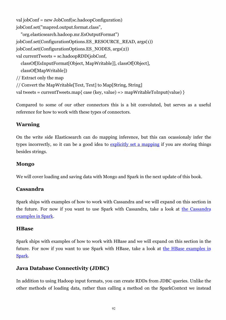
92
val jobConf = new JobConf(sc.hadoopConfiguration)
jobConf.set("mapred.output.format.class",
"org.elasticsearch.hadoop.mr.EsOutputFormat")
jobConf.set(ConfigurationOptions.ES_RESOURCE_READ, args(1))
jobConf.set(ConfigurationOptions.ES_NODES, args(2))
val currentTweets = sc.hadoopRDD(jobConf,
classOf[EsInputFormat[Object, MapWritable]], classOf[Object],
classOf[MapWritable])
// Extract only the map
// Convert the MapWritable[Text, Text] to Map[String, String]
val tweets = currentTweets.map{ case (key, value) => mapWritableToInput(value) }
Compared to some of our other connectors this is a bit convoluted, but serves as a useful
reference for how to work with these types of connectors.
Warning
On the write side Elasticsearch can do mapping inference, but this can ocassionaly infer the
types incorrectly, so it can be a good idea to explicitly set a mapping if you are storing things
besides strings.
Mongo
We will cover loading and saving data with Mongo and Spark in the next update of this book.
Cassandra
Spark ships with examples of how to work with Cassandra and we will expand on this section in
the future. For now if you want to use Spark with Cassandra, take a look at the Cassandra
examples in Spark.
HBase
Spark ships with examples of how to work with HBase and we will expand on this section in the
future. For now if you want to use Spark with HBase, take a look at the HBase examples in
Spark.
Java Database Connectivity (JDBC)
In addition to using Hadoop input formats, you can create RDDs from JDBC queries. Unlike the
other methods of loading data, rather than calling a method on the SparkContext we instead
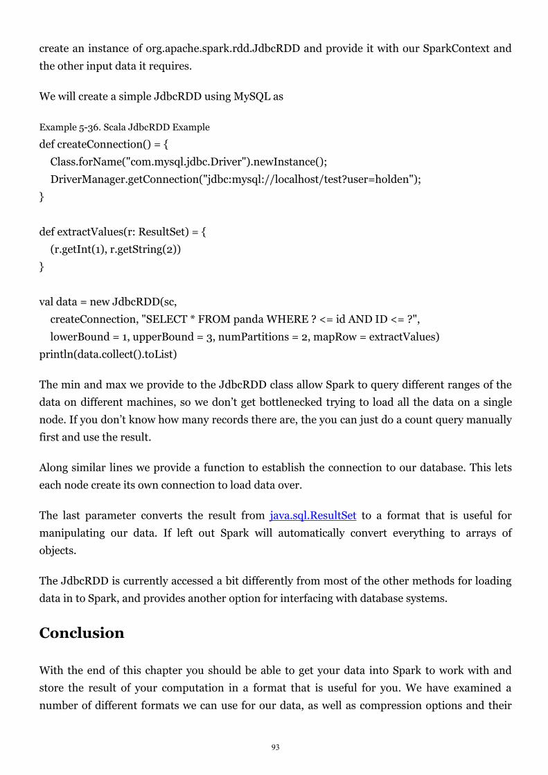
93
create an instance of org.apache.spark.rdd.JdbcRDD and provide it with our SparkContext and
the other input data it requires.
We will create a simple JdbcRDD using MySQL as
Example 5-36. Scala JdbcRDD Example
def createConnection() = {
Class.forName("com.mysql.jdbc.Driver").newInstance();
DriverManager.getConnection("jdbc:mysql://localhost/test?user=holden");
}
def extractValues(r: ResultSet) = {
(r.getInt(1), r.getString(2))
}
val data = new JdbcRDD(sc,
createConnection, "SELECT * FROM panda WHERE ? <= id AND ID <= ?",
lowerBound = 1, upperBound = 3, numPartitions = 2, mapRow = extractValues)
println(data.collect().toList)
The min and max we provide to the JdbcRDD class allow Spark to query different ranges of the
data on different machines, so we don’t get bottlenecked trying to load all the data on a single
node. If you don’t know how many records there are, the you can just do a count query manually
first and use the result.
Along similar lines we provide a function to establish the connection to our database. This lets
each node create its own connection to load data over.
The last parameter converts the result from java.sql.ResultSet to a format that is useful for
manipulating our data. If left out Spark will automatically convert everything to arrays of
objects.
The JdbcRDD is currently accessed a bit differently from most of the other methods for loading
data in to Spark, and provides another option for interfacing with database systems.
Conclusion
With the end of this chapter you should be able to get your data into Spark to work with and
store the result of your computation in a format that is useful for you. We have examined a
number of different formats we can use for our data, as well as compression options and their

94
implications on how data can be consumed. Subsequent chapters will examine ways to write
more effective and powerful Spark programs now that we can load and save large data sets.
[10] sometimes called pbs or protobufs

95
About the Authors
Holden Karau is a software development engineer at Databricks and is active in open source.
She is the author of an earlier Spark book. Prior to Databricks she worked on a variety of search
and classification problems at Google, Foursquare, and Amazon. She graduated from the
University of Waterloo with a Bachelors of Mathematics in Computer Science. Outside of
software she enjoys paying with fire, welding, and hula hooping.
Most recently, Andy Konwinski co-founded Databricks. Before that he was a PhD student and
then postdoc in the AMPLab at UC Berkeley, focused on large scale distributed computing and
cluster scheduling. He co-created and is a committer on the Apache Mesos project. He also
worked with systems engineers and researchers at Google on the design of Omega, their next
generation cluster scheduling system. More recently, he developed and led the AMP Camp Big
Data Bootcamps and first Spark Summit, and has been contributing to the Spark project.
Patrick Wendell is an engineer at Databricks as well as a Spark Committer and PMC member. In
the Spark project, Patrick has acted as release manager for several Spark releases, including
Spark 1.0. Patrick also maintains several subsystems of Spark's core engine. Before helping start
Databricks, Patrick obtained an M.S. in Computer Science at UC Berkeley. His research focused
on low latency scheduling for large scale analytics workloads. He holds a B.S.E in Computer
Science from Princeton University
Matei Zaharia is a PhD student in the AMP Lab at UC Berkeley, working on topics in computer
systems, cloud computing and big data. He is also a committer on Apache Hadoop and Apache
Mesos. At Berkeley, he leads the development of the Spark cluster computing framework, and
has also worked on projects including Mesos, the Hadoop Fair Scheduler, Hadoop's straggler
detection algorithm, Shark, and multi-resource sharing. Matei got his undergraduate degree at
the University of Waterloo in Canada.