learning structured predictors - lxmls 2020lxmls.it.pt/2018/strlearn.pdf · 2018-06-19 · learning...
TRANSCRIPT


Supervised (Structured) Prediction
I Learning to predict: given training data{(x(1),y(1)), (x(2),y(2)), . . . , (x(m),y(m))
}
learn a predictor x→ y that works well on unseen inputs x
I Non-Structured Prediction: outputs y are atomicI Binary prediction: y ∈ {−1,+1}I Multiclass prediction: y ∈ {1, 2, . . . , L}
I Structured Prediction: outputs y are structuredI Sequence prediction: y are sequencesI Parsing: y are treesI . . .
2/74

Named Entity Recognition
y per - qnt - - org org - timex Jim bought 300 shares of Acme Corp. in 2006
y per per - - locx Jack London went to Paris
y per per - - locx Paris Hilton went to London
y per - - locx Jackie went to Lisdon
3/74

Named Entity Recognition
y per - qnt - - org org - timex Jim bought 300 shares of Acme Corp. in 2006
y per per - - locx Jack London went to Paris
y per per - - locx Paris Hilton went to London
y per - - locx Jackie went to Lisdon
3/74

Part-of-speech Tagging
y NNP NNP VBZ NNP .x Ms. Haag plays Elianti .
4/74

Syntactic Parsing
? Unesco is now holding its biennial meetings in New York .
ROOT
SBJ TMP
VC NMOD
NMOD
OBJ
LOC
NAME
PMOD
P
x are sentencesy are syntactic dependency trees
5/74

Machine Translation
rules may describe the transformation of does notinto ne ... pas in French. A particular instance maylook like this:
VP(AUX(does), RB(not), x0:VB)→ ne, x0, pas
lhs(ri) can be any arbitrary syntax tree fragment.Its leaves are either lexicalized (e.g. does) or vari-ables (x0, x1, etc). rhs(ri) is represented as a se-quence of target-language words and variables.
Now we give a brief overview of how suchtransformational rules are acquired automaticallyin GHKM.1 In Figure 1, the (π, f ,a) triple is rep-resented as a directed graph G (edges going down-ward), with no distinction between edges of π andalignments. Each node of the graph is labeled withits span and complement span (the latter in italicin the figure). The span of a node n is defined bythe indices of the first and last word in f that arereachable from n. The complement span of n isthe union of the spans of all nodes n� in G thatare neither descendants nor ancestors of n. Nodesof G whose spans and complement spans are non-overlapping form the frontier set F ∈ G.
What is particularly interesting about the fron-tier set? For any frontier of graph G containinga given node n ∈ F , spans on that frontier de-fine an ordering between n and each other frontiernode n�. For example, the span of VP[4-5] eitherprecedes or follows, but never overlaps the span ofany node n� on any graph frontier. This propertydoes not hold for nodes outside of F . For instance,PP[4-5] and VBG[4] are two nodes of the samegraph frontier, but they cannot be ordered becauseof their overlapping spans.
The purpose of xRs rules in this framework isto order constituents along sensible frontiers in G,and all frontiers containing undefined orderings,as between PP[4-5] and VBG[4], must be disre-garded during rule extraction. To ensure that xRsrules are prevented from attempting to re-orderany such pair of constituents, these rules are de-signed in such a way that variables in their lhs canonly match nodes of the frontier set. Rules thatsatisfy this property are said to be induced by G.2
For example, rule (d) in Table 1 is valid accord-ing to GHKM, since the spans corresponding to
1Note that we use a slightly different terminology.2Specifically, an xRs rule ri is extracted from G by taking
a subtree γ ∈ π as lhs(ri), appending a variable to eachleaf node of γ that is internal to π, adding those variables torhs(ri), ordering them in accordance to a, and if necessaryinserting any word of f to ensure that rhs(ri) is a sequence ofcontiguous spans (e.g., [4-5][6][7-8] for rule (f) in Table 1).
!" #! $%& ''( )' ''&
'&
''( $%*
!""# $%& ' ' ( )
# " ! ' ( * $ & )
!!"#$%"&
"!"&
"!"&
##"&
$%&!"'$&
'!"&
'!"&
(!"%$("&
)!")
#%"*"&
'&$%&!"'$&
'&(
!"%$+("&
&&'%(
!"%$("&
$&'%(
!"*$("&
'&'%&!"*$&
$&!%&!"#$&
(#%)!
!! "#$ %& '( ) *+ , "
"#$%$ &$'&($ )*+(,-$ .%/0'*.,/% +'1)*2 30'1 40.*+$ +
+
5
-
Figure 1: Spans and complement-spans determine whatrules are extracted. Constituents in gray are members of thefrontier set; a minimal rule is extracted from each of them.
(a) S(x0:NP, x1:VP, x2:.) → x0, x1, x2
(b) NP(x0:DT, CD(7), NNS(people))→ x0, 7(c) DT(these)→(d) VP(x0:VBP, x1:NP)→ x0, x1
(e) VBP(include)→(f) NP(x0:NP, x1:VP)→ x1, , x0
(g) NP(x0:NNS)→ x0
(h) NNS(astronauts)→ ,(i) VP(VBG(coming), PP(IN(from), x0:NP))→ , x0
(j) NP(x0:NNP)→ x0
(k) NNP(France)→(l) .(.) → .
Table 1: A minimal derivation corresponding to Figure 1.
its rhs constituents (VBP[3] and NP[4-8]) do notoverlap. Conversely, NP(x0:DT, x1:CD:, x2:NNS)is not the lhs of any rule extractible from G, sinceits frontier constituents CD[2] and NNS[2] haveoverlapping spans.3 Finally, the GHKM proce-dure produces a single derivation from G, whichis shown in Table 1.
The concern in GHKM was to extract minimalrules, whereas ours is to extract rules of any arbi-trary size. Minimal rules defined over G are thosethat cannot be decomposed into simpler rules in-duced by the same graph G, e.g., all rules in Ta-ble 1. We call minimal a derivation that only con-tains minimal rules. Conversely, a composed ruleresults from the composition of two or more min-imal rules, e.g., rule (b) and (c) compose into:
NP(DT(these), CD(7), NNS(people))→ , 7
3It is generally reasonable to also require that the root nof lhs(ri) be part of F , because no rule induced by G cancompose with ri at n, due to the restrictions imposed on theextraction procedure, and ri wouldn’t be part of any validderivation.
(Galley, Graehl, Knight, Marcu, DeNeefe, Wang, and Thayer, 2006)
x are sentences in Chinesey are sentences in English aligned to x
6/74

Object Detection
(Kumar and Hebert, 2003)
x are imagesy are grids labeled with object types
7/74

Object Detection
(Kumar and Hebert, 2003)
x are imagesy are grids labeled with object types
7/74

Today’s Goals
I Introduce basic concepts for structured predictionI We will restrict to sequence prediction
I What can we can borrow from standard classification?I Learning paradigms and algorithms, in essence, work here tooI However, computations behind algorithms are prohibitive
I What can we borrow from HMM and other structured formalisms?I Representations of structured data into feature spacesI Inference/search algorithms for tractable computationsI E.g., algorithms for HMMs (Viterbi, forward-backward) will play a major role in today’s
methods
8/74

Sequence Prediction
y per per - - locx Jack London went to Paris
9/74

Sequence Prediction
I x = x1x2 . . . xn are input sequences, xi ∈ XI y = y1y2 . . . yn are output sequences, yi ∈ {1, . . . , L}
I Goal: given training data
{(x(1),y(1)), (x(2),y(2)), . . . , (x(m),y(m))
}
learn a predictor x→ y that works well on unseen inputs x
I What is the form of our prediction model?
10/74

Exponentially-many Solutions
I Let Y = {-,per, loc}
I The solution space (all output sequences):
Jack London went to Paris
-
per
loc
-
per
loc
-
per
loc
-
per
loc
-
per
loc
I Each path is a possible solution
I For an input sequence of size n, there are |Y|n possible outputs
11/74

Exponentially-many Solutions
I Let Y = {-,per, loc}
I The solution space (all output sequences):
Jack London went to Paris
-
per
loc
-
per
loc
-
per
loc
-
per
loc
-
per
loc
I Each path is a possible solution
I For an input sequence of size n, there are |Y|n possible outputs
11/74

Approach 1: Label Classifiers
I Multiclass prediction over individual labels at each position
yi = argmaxl ∈ {loc, per, -}
score(x, i, l)
I For linear models, score(x, i, l) = w · f(x, i, l)I f(x, i, l) ∈ Rd represents an assignment of label l for xiI w ∈ Rd is a vector of parameters (learned), has a weight for each feature in f
I Can capture interactions between full input sequence x and one output label le.g.: current word, surrounding words, capitalization, prefix-suffix, gazetteer, . . .
I Can not capture interactions between output labels!12/74

Approach 2: HMM for Sequence Prediction
perπper
perTper,per
- - loc
Jack London
Oper, London
went to Paris
I Define an HMM were each label is a stateI Model parameters:
I πl : probability of starting with label lI Tl,l′ : probability of transitioning from l to l′
I Ol,x: probability of generating symbol x given label lI Predictions:
p(x,y) = πy1Oy1,x1
∏
i>1
Tyi−1,yiOyi,xi
I Learning: relative counts + smoothingI Prediction: Viterbi algorithm
13/74

Approach 2: Representation in HMM
perπper
perTper,per
- - loc
Jack London
Oper, London
went to Paris
I Label interactions are captured in the transition parametersI But interactions between labels and input symbols are quite limited!
I Only Oyi,xi= p(xi | yi)
I Not clear how to exploit patterns such as:I Capitalization, digitsI Prefixes and suffixesI Next word, previous wordI Combinations of these with label transitions
I Why? HMM independence assumptions:given label yi, token xi is independent of anything else
14/74

Approach 3: Transition-based Sequence Prediction
I Predict one label at a time, left-to-right, using previous predictions:
yi = argmaxl ∈ {loc, per, -}
score(x, i, l, y1:i−1)
I Captures interactions between full input x and prefixes of the output sequence
I Prediction of y is approximate (greedy, beam search)
15/74

Approach 4: Factored Sequence Prediction
I At each position, multiclass prediction over label bigrams (pairs of adjacent labels):
y = argmaxy ∈ Y
score(x,y) = argmaxy ∈ Y
n∑
i=1
score(x, i, yi−1, yi)
I Output sequence factored into label bigrams
I Captures interactions between full input x and label bigrams
I Prediction is tractable for many types of factorizations (this lecture)
16/74

Approach 5: Re-Ranking
y = argmaxy ∈ A(Y)
score(x,y)
I Scoring of full inputs and outputsI Relies on an active set of full outputs, enumerated exhaustivelyI Previous approaches can be used to select active set
17/74

Sequence Prediction: Summary of Approaches
18/74

Factored Sequence Predictors
y = argmaxy ∈ Y
n∑
i=1
score(x, i, yi−1, yi)
Next questions:
I There are exponentially-many sequences y for a given x,how do we solve the argmax problem?
I What is the form of score(x, i, a, b)?We will use linear scoring functions: score(x, i, a, b) = w · f(x, i, a, b)
I How do we learn w?19/74

Predicting with Factored Sequence Models
I Assume we have a score function score(x, i, a, b)
I Given x1:n find:
argmaxy∈Yn
n∑
i=1
score(x, i, yi−1, yi)
I Use the Viterbi algorithm, takes O(n|Y|2)
I Notational change: since x1:n is fixed we will use
s(i, a, b) = score(x, i, a, b)
20/74

Viterbi for Factored Sequence Models
I Given scores s(i, a, b) for each position i and output bigram a, b, find:
argmaxy∈Yn
n∑
i=1
s(i, yi−1, yi)
I Use the Viterbi algorithm, takes O(n|Y|2)
I Intuition: output sequences that share bigrams will share scores1 . . . i− 2 i− 1 i i+ 1 . . . n
best subsequence with yi−1 = per
best subsequence with yi−1 = loc
best subsequence with yi−1 = –
best subsequence with yi = per
s(i,lo
c,per
)
best subsequence with yi = loc
best subsequence with yi = –
21/74

Intuition for Viterbi
I Assume we have the best sub-sequence up to position i− 1 ending with each label:
1 . . . i− 1 i
best subsequence with yi−1 = per
best subsequence with yi−1 = loc
best subsequence with yi−1 = –
s(i,per, loc)
s(i,loc, loc)
s(i,–, lo
c)
I What is the best sequence up to position i with yi =loc?
22/74
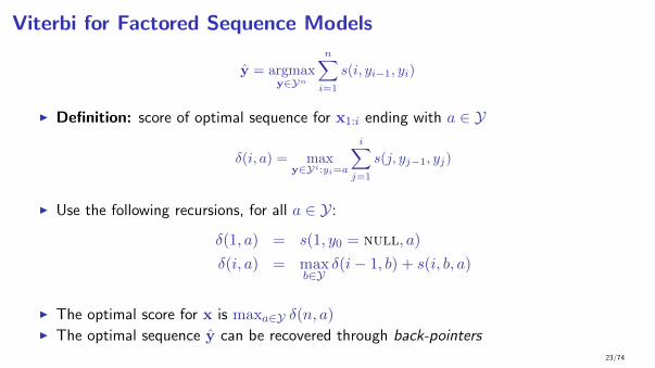
Viterbi for Factored Sequence Models
y = argmaxy∈Yn
n∑
i=1
s(i, yi−1, yi)
I Definition: score of optimal sequence for x1:i ending with a ∈ Y
δ(i, a) = maxy∈Yi:yi=a
i∑
j=1
s(j, yj−1, yj)
I Use the following recursions, for all a ∈ Y:
δ(1, a) = s(1, y0 = null, a)
δ(i, a) = maxb∈Y
δ(i− 1, b) + s(i, b, a)
I The optimal score for x is maxa∈Y δ(n, a)I The optimal sequence y can be recovered through back-pointers
23/74

Linear Factored Models and Representations
argmaxy ∈ Y
n∑
i=1
score(x, i, yi−1, yi)
I In linear factored models:
score(x, i, a, b) = w · f(x, i, a, b)
I w ∈ Rd is a parameter vector, to be learned
I f(x, i, a, b) ∈ Rd is a feature vectorI How to construct f(x, i, a, b)?
I New trend: representation learningI Old school: manually with feature templates
24/74
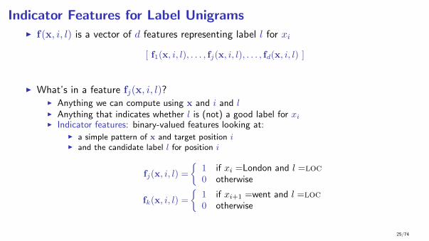
Indicator Features for Label UnigramsI f(x, i, l) is a vector of d features representing label l for xi
[ f1(x, i, l), . . . , fj(x, i, l), . . . , fd(x, i, l) ]
I What’s in a feature fj(x, i, l)?I Anything we can compute using x and i and lI Anything that indicates whether l is (not) a good label for xiI Indicator features: binary-valued features looking at:
I a simple pattern of x and target position iI and the candidate label l for position i
fj(x, i, l) =
{1 if xi =London and l =loc0 otherwise
fk(x, i, l) =
{1 if xi+1 =went and l =loc0 otherwise
25/74

Feature TemplatesI Feature templates generate many indicator features mechanicallyI A feature template is identified by a type, and a number of values
I Example: template word indicates the current word
f〈word,a,w〉(x, i, l) =
{1 if xi = w and l = a0 otherwise
I A feature of this type is identified by the tuple 〈word, a, w〉I Generates a feature for every label a ∈ Y and every word w
e.g.: a = loc w = London, a = - w = Londona = loc w = Paris a = per w = Parisa = per w = John a = - w = the
I In feature-based models:I Define feature templates manuallyI Instantiate the templates on every set of values in the training data→ generates a very high-dimensional feature space
I Define parameter vector w indexed by such feature tuplesI Let the learning algorithm choose the relevant features
26/74

More Features for NE Recognition
per
-
Jack London went to Paris
In practice, construct f(x, i, l) by . . .
I Define a number of simple patterns of x and i
I current word xiI is xi capitalized?I xi has digits?I prefixes/suffixes of size 1, 2, 3, . . .I is xi a known location?I is xi a known person?
I next wordI previous wordI current and next words togetherI other combinations
I Define feature templates by combining patterns with labels l
I Generate actual features by instantiating templates on training data
27/74

More Features for NE Recognition
per -Jack London went to Paris
In practice, construct f(x, i, l) by . . .
I Define a number of simple patterns of x and i
I current word xiI is xi capitalized?I xi has digits?I prefixes/suffixes of size 1, 2, 3, . . .I is xi a known location?I is xi a known person?
I next wordI previous wordI current and next words togetherI other combinations
I Define feature templates by combining patterns with labels l
I Generate actual features by instantiating templates on training data
27/74

Bigram Feature Templates1 2 3 4 5
y per per - - locx Jack London went to Paris
I Example: A template for word + bigram:
f〈wb,a,b,w〉(x, i, yi−1, yi) =
1 if xi = w andyi−1 = a and yi = b
0 otherwise
e.g., f〈wb,per,per,London〉(x, 2,per,per) = 1
f〈wb,per,per,London〉(x, 3,per, -) = 0
f〈wb,per,-,went〉(x, 3,per, -) = 1
I Bigram feature templates are strictly more expressive than unigram templates28/74

More Templates for NER1 2 3 4 5
x Jack London went to Parisy per per - - locy′ per loc - - locy′′ - - - loc -x′ My trip to London . . .
f〈w,per,per,London〉(. . .) = 1 iff xi =”London” and yi−1 = per and yi = per
f〈w,per,loc,London〉(. . .) = 1 iff xi =”London” and yi−1 = per and yi = loc
f〈prep,loc,to〉(. . .) = 1 iff xi−1 =”to” and xi ∼/[A-Z]/ and yi = loc
f〈city,loc〉(. . .) = 1 iff yi = loc and world-cities(xi) = 1
f〈fname,per〉(. . .) = 1 iff yi = per and first-names(xi) = 1
29/74

Representations Factored at Bigrams
y: per per - - locx: Jack London went to Paris
I f(x, i, yi−1, yi)I A d-dimensional feature vector of a label bigram at iI Each dimension is typically a boolean indicator (0 or 1)
I f(x,y) =∑n
i=1 f(x, i, yi−1, yi)I A d-dimensional feature vector of the entire yI Aggregated representation by summing bigram feature vectorsI Each dimension is now a count of a feature pattern
30/74

Linear Factored Sequence Prediction
argmaxy∈Yn
w · f(x,y)
wheref(x,y) =
n∑
i=1
f(x, i, yi−1, yi)
I Note the linearity of the expression:
w · f(x,y) = w ·n∑
i=1
f(x, i, yi−1, yi)
=
n∑
i=1
w · f(x, i, yi−1, yi)
=
n∑
i=1
score(x, i, yi−1, yi)
31/74

Linear Factored Sequence Prediction
argmaxy∈Yn
w · f(x,y)
I Factored representation, e.g. based on bigrams
I Flexible, arbitrary features of full x and the factors
I Efficient prediction using ViterbiI Next, learning w:
I Probabilistic log-linear models:I Local learning, a.k.a. Maximum-Entropy Markov ModelsI Global learning, a.k.a. Conditional Random Fields
I Margin-based methods:I Structured PerceptronI Structured SVM
32/74

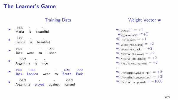
The Learner’s Game
Training Data
I per - -Maria is beautiful
I loc - -Lisbon is beautiful
I per - - locJack went to Lisbon
I loc - -Argentina is nice
I per per - - loc locJack London went to South Paris
I org - - orgArgentina played against Iceland
Weight Vector w
w〈Lower,-〉 = +1
w〈Upper,loc〉 = +1w〈Word,per,Maria〉 = +2w〈Word,per,Jack〉 = +2w〈NextW,per,went〉 = +2w〈NextW,org,played〉 = +2w〈PrevW,org,against〉 = +2. . .w〈UpperBigram,per,per〉 = +2w〈UpperBigram,loc,loc〉 = +2w〈NextW,loc,played〉 = −1000
33/74

The Learner’s Game
Training Data
I per - -Maria is beautiful
I loc - -Lisbon is beautiful
I per - - locJack went to Lisbon
I loc - -Argentina is nice
I per per - - loc locJack London went to South Paris
I org - - orgArgentina played against Iceland
Weight Vector w
w〈Lower,-〉 = +1w〈Upper,per〉 = +1
w〈Upper,loc〉 = +1w〈Word,per,Maria〉 = +2w〈Word,per,Jack〉 = +2w〈NextW,per,went〉 = +2w〈NextW,org,played〉 = +2w〈PrevW,org,against〉 = +2. . .w〈UpperBigram,per,per〉 = +2w〈UpperBigram,loc,loc〉 = +2w〈NextW,loc,played〉 = −1000
33/74

The Learner’s Game
Training Data
I per - -Maria is beautiful
I loc - -Lisbon is beautiful
I per - - locJack went to Lisbon
I loc - -Argentina is nice
I per per - - loc locJack London went to South Paris
I org - - orgArgentina played against Iceland
Weight Vector w
w〈Lower,-〉 = +1
((((((((w〈Upper,per〉 = +1w〈Upper,loc〉 = +1
w〈Word,per,Maria〉 = +2w〈Word,per,Jack〉 = +2w〈NextW,per,went〉 = +2w〈NextW,org,played〉 = +2w〈PrevW,org,against〉 = +2. . .w〈UpperBigram,per,per〉 = +2w〈UpperBigram,loc,loc〉 = +2w〈NextW,loc,played〉 = −1000
33/74

The Learner’s Game
Training Data
I per - -Maria is beautiful
I loc - -Lisbon is beautiful
I per - - locJack went to Lisbon
I loc - -Argentina is nice
I per per - - loc locJack London went to South Paris
I org - - orgArgentina played against Iceland
Weight Vector w
w〈Lower,-〉 = +1
((((((((w〈Upper,per〉 = +1w〈Upper,loc〉 = +1w〈Word,per,Maria〉 = +2
w〈Word,per,Jack〉 = +2w〈NextW,per,went〉 = +2w〈NextW,org,played〉 = +2w〈PrevW,org,against〉 = +2. . .w〈UpperBigram,per,per〉 = +2w〈UpperBigram,loc,loc〉 = +2w〈NextW,loc,played〉 = −1000
33/74

The Learner’s Game
Training Data
I per - -Maria is beautiful
I loc - -Lisbon is beautiful
I per - - locJack went to Lisbon
I loc - -Argentina is nice
I per per - - loc locJack London went to South Paris
I org - - orgArgentina played against Iceland
Weight Vector w
w〈Lower,-〉 = +1
((((((((w〈Upper,per〉 = +1w〈Upper,loc〉 = +1w〈Word,per,Maria〉 = +2w〈Word,per,Jack〉 = +2
w〈NextW,per,went〉 = +2w〈NextW,org,played〉 = +2w〈PrevW,org,against〉 = +2. . .w〈UpperBigram,per,per〉 = +2w〈UpperBigram,loc,loc〉 = +2w〈NextW,loc,played〉 = −1000
33/74

The Learner’s Game
Training Data
I per - -Maria is beautiful
I loc - -Lisbon is beautiful
I per - - locJack went to Lisbon
I loc - -Argentina is nice
I per per - - loc locJack London went to South Paris
I org - - orgArgentina played against Iceland
Weight Vector w
w〈Lower,-〉 = +1
((((((((w〈Upper,per〉 = +1w〈Upper,loc〉 = +1w〈Word,per,Maria〉 = +2w〈Word,per,Jack〉 = +2w〈NextW,per,went〉 = +2
w〈NextW,org,played〉 = +2w〈PrevW,org,against〉 = +2. . .w〈UpperBigram,per,per〉 = +2w〈UpperBigram,loc,loc〉 = +2w〈NextW,loc,played〉 = −1000
33/74

The Learner’s Game
Training Data
I per - -Maria is beautiful
I loc - -Lisbon is beautiful
I per - - locJack went to Lisbon
I loc - -Argentina is nice
I per per - - loc locJack London went to South Paris
I org - - orgArgentina played against Iceland
Weight Vector w
w〈Lower,-〉 = +1
((((((((w〈Upper,per〉 = +1w〈Upper,loc〉 = +1w〈Word,per,Maria〉 = +2w〈Word,per,Jack〉 = +2w〈NextW,per,went〉 = +2w〈NextW,org,played〉 = +2
w〈PrevW,org,against〉 = +2. . .w〈UpperBigram,per,per〉 = +2w〈UpperBigram,loc,loc〉 = +2w〈NextW,loc,played〉 = −1000
33/74

The Learner’s Game
Training Data
I per - -Maria is beautiful
I loc - -Lisbon is beautiful
I per - - locJack went to Lisbon
I loc - -Argentina is nice
I per per - - loc locJack London went to South Paris
I org - - orgArgentina played against Iceland
Weight Vector w
w〈Lower,-〉 = +1
((((((((w〈Upper,per〉 = +1w〈Upper,loc〉 = +1w〈Word,per,Maria〉 = +2w〈Word,per,Jack〉 = +2w〈NextW,per,went〉 = +2w〈NextW,org,played〉 = +2w〈PrevW,org,against〉 = +2
. . .w〈UpperBigram,per,per〉 = +2w〈UpperBigram,loc,loc〉 = +2w〈NextW,loc,played〉 = −1000
33/74
The Learner’s Game
Training Data
I per - -Maria is beautiful
I loc - -Lisbon is beautiful
I per - - locJack went to Lisbon
I loc - -Argentina is nice
I per per - - loc locJack London went to South Paris
I org - - orgArgentina played against Iceland
Weight Vector w
w〈Lower,-〉 = +1
((((((((w〈Upper,per〉 = +1w〈Upper,loc〉 = +1w〈Word,per,Maria〉 = +2w〈Word,per,Jack〉 = +2w〈NextW,per,went〉 = +2w〈NextW,org,played〉 = +2w〈PrevW,org,against〉 = +2. . .w〈UpperBigram,per,per〉 = +2w〈UpperBigram,loc,loc〉 = +2w〈NextW,loc,played〉 = −1000
33/74
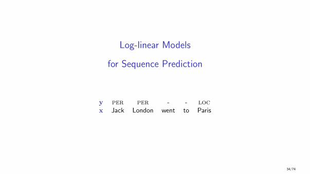
Log-linear Models
for Sequence Prediction
y per per - - locx Jack London went to Paris
34/74

Log-linear Models for Sequence PredictionI Model the conditional distribution:
Pr(y | x;w) =exp {w · f(x,y)}
Z(x;w)
whereI x = x1x2 . . . xn ∈ X ∗I y = y1y2 . . . yn ∈ Y∗ and Y = {1, . . . , L}I f(x,y) represents x and y with d featuresI w ∈ Rd are the parameters of the modelI Z(x;w) is a normalizer called the partition function
Z(x;w) =∑
z∈Y∗exp {w · f(x, z)}
I To predict the best sequenceargmaxy∈Yn
Pr(y|x)
35/74

Log-linear Models: Name
I Let’s take the log of the conditional probability:
log Pr(y | x;w) = logexp{w · f(x,y)}
Z(x;w)
= w · f(x,y)− log∑
y
exp{w · f(x,y)}
= w · f(x,y)− logZ(x;w)
I Partition function: Z(x;w) =∑
y exp{w · f(x,y)}I logZ(x;w) is a constant for a fixed x
I In the log space, computations are linear,i.e., we model log-probabilities using a linear predictor
36/74

Making Predictions with Log-Linear ModelsI For tractability, assume f(x,y) decomposes into bigrams:
f(x1:n,y1:n) =
n∑
i=1
f(x, i, yi−1, yi)
I Given w, given x1:n, find:
argmaxy1:n
Pr(y1:n|x1:n;w) = amaxy
exp {∑ni=1w · f(x, i, yi−1, yi)}
Z(x;w)
= amaxy
exp
{n∑
i=1
w · f(x, i, yi−1, yi)}
= amaxy
n∑
i=1
w · f(x, i, yi−1, yi)
I We can use the Viterbi algorithm37/74

Parameter Estimation in Log-Linear Models
Pr(y | x;w) =exp {w · f(x,y)}
Z(x;w)
I Given training data{(x(1),y(1)), (x(2),y(2)), . . . , (x(m),y(m))
},
I How to estimate w?I Define the conditional log-likelihood of the data:
L(w) =∑
a
k = 1m log Pr(y(k)|x(k);w)
I L(w) measures how well w explains the data. A good value for w will give a highvalue for Pr(y(k)|x(k);w) for all k = 1 . . .m.
I We want w that maximizes L(w)38/74

Learning Log-Linear Models: Loss + Regularization
I Solve:
w∗ = argminw∈Rd
Loss︷ ︸︸ ︷−L(w)+
Regularization︷ ︸︸ ︷λ
2||w||2
whereI The first term is the negative conditional log-likelihoodI The second term is a regularization term, it penalizes solutions with large normI λ ∈ R controls the trade-off between loss and regularization
I Convex optimization problem → gradient descentI Two common losses based on log-likelihood that make learning tractable:
I Local Loss (MEMM): assume that Pr(y | x;w) decomposesI Global Loss (CRF): assume that f(x,y) decomposes
39/74

Maximum Entropy Markov Models (MEMM)McCallum, Freitag, and Pereira (2000)
I Similarly to HMMs:
Pr(y1:n | x1:n) = Pr(y1 | x1:n)× Pr(y2:n | x1:n, y1)
= Pr(y1 | x1:n)×n∏
i=2
Pr(yi|x1:n,y1:i−1)
= Pr(y1|x1:n)×n∏
i=2
Pr(yi|x1:n,yi−1)
I Assumption under MEMMs:
Pr(yi|x1:n,y1:i−1) = Pr(yi|x1:n, yi−1)
40/74

Parameter Estimation in MEMM
Pr(y1:n | x1:n) = Pr(y1 | x1:n)×n∏
i=2
Pr(yi|x1:n, i, yi−1)
I The log-linear model is normalized locally (i.e. at each position):
Pr(y | x, i, y′) = exp{w · f(x, i, y′, y)}Z(x, i, y′)
I The log-likelihood is also local :
L(w) =
m∑
k=1
n(k)∑
i=1
log Pr(y(k)i |x(k), i,y
(k)i−1)
∂L(w)
∂wj=
1
m
m∑
k=1
n(k)∑
i=1
observed︷ ︸︸ ︷fj(x
(k), i,y(k)i−1,y
(k)i )−
expected︷ ︸︸ ︷∑
y∈YPr(y|x(k), i,y
(k)i−1, y) fj(x
(k), i,y(k)i−1, y)
41/74

Conditional Random FieldsLafferty, McCallum, and Pereira (2001)
I Log-linear model of the conditional distribution:
Pr(y|x;w) =exp{w · f(x,y)}
Z(x)
whereI x and y are input and output sequencesI f(x,y) is a feature vector of x and y that decomposes into factorsI w are model parameters
I To predict the best sequence
y = argmaxy∈Y∗
Pr(y|x)
I Log-Likelihood at the global (sequence) level:
L(w) =
m∑
k=1
log Pr(y(k)|x(k);w)
42/74

Computing the Gradient in CRFs
Consider a parameter wj and its associated feature fj :
∂L(w)
∂wj=
1
m
m∑
k=1
observed︷ ︸︸ ︷fj(x
(k),y(k))−
expected︷ ︸︸ ︷∑
y∈Y∗Pr(y|x(k);w) fj(x
(k),y)
where
fj(x,y) =
n∑
i=1
fj(x, i, yi−1, yi)
I First term: observed value of fj in training examples
I Second term: expected value of fj under current w
I In the optimal, observed = expected
43/74
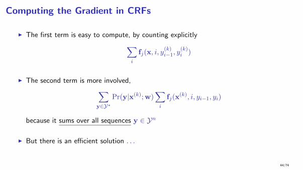
Computing the Gradient in CRFs
I The first term is easy to compute, by counting explicitly
∑
i
fj(x, i, y(k)i−1, y
(k)i )
I The second term is more involved,
∑
y∈Y∗Pr(y|x(k);w)
∑
i
fj(x(k), i, yi−1, yi)
because it sums over all sequences y ∈ Yn
I But there is an efficient solution . . .
44/74

Computing the Gradient in CRFs
I For an example (x(k),y(k)):
∑
y∈Yn
Pr(y|x(k);w)
n∑
i=1
fj(x(k), i, yi−1, yi) =
n∑
i=1
∑
a,b∈Yµki (a, b)fj(x
(k), i, a, b)
I µki (a, b) is the marginal probability of having labels (a, b) at position i:
µki (a, b) =Pr(〈i, a, b〉 | x(k);w) =∑
y∈Yn : yi−1=a, yi=b
Pr(y|x(k);w)
I The quantities µki can be computed efficiently in O(nL2) using the forward-backwardalgorithm
45/74

Forward-Backward for CRFs
I Assume fixed x and w.
I For notational convenience, define the score of a label bigram as:
s(i, a, b) = exp{w · f(x, i, a, b)}
such that we can write
Pr(y | x) = exp{w · f(x,y)}Z(x)
=exp{∑n
i=1w · f(x, i, yi−1, yi)}Z(x)
=
∏ni=1 s(i, yi−1, yi)
Z
I Normalizer: Z =∑
y
∏ni=1 s(i, yi−1, yi)
I Marginals: µ(i, a, b) = 1Z
∑y,s.t.yi−1=a,yi=b
∏ni=1 s(i, yi−1, yi)
46/74

Forward-Backward for CRFs
I Definition: forward and backward quantities
αi(a) =∑
y1:i∈Yi:yi=a
∏ij=1 s(j, yj−1, yj)
βi(b) =∑
yi:n∈Y(n−i+1):yi=b
∏nj=i+1 s(j, yj−1, yj)
I Z =∑
a αn(a)
I µi(a, b) = {αi−1(a) ∗ s(i, a, b)} ∗ βi(b) ∗ Z−1}
I Similarly to Viterbi, αi(a) and βi(b) can be computed recursively in O(n|Y|2)
47/74

CRFs: summary so far
I Log-linear models for sequence prediction, Pr(y|x;w)
I Computations factorize on label bigrams
I Model form:argmaxy∈Y∗
∑
i
w · f(x, i, yi−1, yi)
I Prediction: uses Viterbi (from HMMs)I Parameter estimation:
I Gradient-based methods, in practice L-BFGSI Computation of gradient uses forward-backward (from HMMs)
48/74

CRFs: summary so far
I Log-linear models for sequence prediction, Pr(y|x;w)
I Computations factorize on label bigrams
I Model form:argmaxy∈Y∗
∑
i
w · f(x, i, yi−1, yi)
I Prediction: uses Viterbi (from HMMs)I Parameter estimation:
I Gradient-based methods, in practice L-BFGSI Computation of gradient uses forward-backward (from HMMs)
I Next Question: MEMMs or CRFs? HMMs or CRFs?
48/74

MEMMs and CRFs
MEMMs: Pr(y | x) =n∏
i=1
exp {w · f(x, i, yi−1, yi)}Z(x, i, yi−1;w)
CRFs: Pr(y | x) = exp {∑ni=1 w · f(x, i, yi−1, yi)}
Z(x)
I Both exploit the same factorization, i.e. same features
I Same computations to compute argmaxy Pr(y | x)I MEMMs locally normalized; CRFs globally normalized
I MEMM assume that Pr(yi | x1:n, y1:i−1) = Pr(yi | x1:n, yi−1)I Leads to “Label Bias Problem” (Lafferty et al., 2001; Andor et al., 2016)
I MEMMs are cheaper to train (reduces to multiclass learning)
I CRFs are easier to extend to other structures (next lecture)
49/74

HMMs for sequence prediction
I x are the observations, y are the hidden states
I HMMs model the joint distributon Pr(x,y)
I Parameters: (assume X = {1, . . . , k} and Y = {1, . . . , l})I π ∈ Rl, πa = Pr(y1 = a)I T ∈ Rl×l, Ta,b = Pr(yi = b|yi−1 = a)I O ∈ Rl×k, Oa,c = Pr(xi = c|yi = a)
I Model form
Pr(x,y) = πy1Oy1,x1
n∏
i=2
Tyi−1,yiOyi,xi
I Parameter Estimation: maximum likelihood by counting events and normalizing
50/74

HMMs and CRFs
I In CRFs: y = amaxy∑
iw · f(x, i, yi−1, yi)
I In HMMs:y = amaxy πy1Oy1,x1
∏ni=2 Tyi−1,yiOyi,xi
= amaxy log(πy1Oy1,x1) +∑n
i=2 log(Tyi−1,yiOyi,xi)
I An HMM can be expressed as factored linear models:
fj(x, i, y, y′) wj
i = 1 & y′ = a log(πa)i > 1 & y = a & y′ = b log(Ta,b)
y′ = a & xi = c log(Oa,b)
I Hence, HMM are factored linear models
51/74

HMMs and CRFs: main differences
I Representation:I HMM “features” are tied to the generative process.I CRF features are very flexible. They can look at the whole input x paired with a label
bigram (yi, yi+1).I In practice, for prediction tasks, “good” discriminative features can improve accuracy a
lot.
I Parameter estimation:I HMMs focus on explaining the data, both x and y.I CRFs focus on the mapping from x to y.I A priori, it is hard to say which paradigm is better.I Same dilemma as Naive Bayes vs. Maximum Entropy.
52/74

Structured Prediction
Perceptron, SVMs, CRFs
53/74

Learning Structured Predictors
I Goal: given training data{(x(1),y(1)), (x(2),y(2)), . . . , (x(m),y(m))
}
learn a predictor x→ y with small error on unseen inputs
I In a CRF:argmaxy∈Y∗
P (y|x;w) =exp {∑n
i=1w · f(x, i, yi−1, yi)}Z(x;w)
=
n∑
i=1
w · f(x, i, yi−1, yi)
I To predict new values, Z(x;w) is not relevantI Parameter estimation: w is set to maximize likelihood
I Can we learn w more directly, focusing on errors?
54/74

The Structured PerceptronCollins (2002)
I Set w = 0
I For t = 1 . . . TI For each training example (x,y)
1. Compute z = argmaxz w · f(x, z)2. If z 6= y
w← w + f(x,y)− f(x, z)
I Return w
55/74

The Structured Perceptron + AveragingFreund and Schapire (1999); Collins (2002)
I Set w = 0, wa = 0
I For t = 1 . . . TI For each training example (x,y)
1. Compute z = argmaxz w · f(x, z)2. If z 6= y
w← w + f(x,y)− f(x, z)
3. wa = wa +w
I Return wa/mT , where m is the number of training examples
56/74

Perceptron Updates: Example
y per per - - locz per loc - - locx Jack London went to Paris
I Let y be the correct output for x.I Say we predict z instead, under our current wI The update is:
g = f(x,y)− f(x, z)
=∑
i
f(x, i, yi−1, yi)−∑
i
f(x, i, zi−1, zi)
= f(x, 2,per,per)− f(x, 2,per, loc)
+ f(x, 3,per, -)− f(x, 3, loc, -)
I Perceptron updates are typically very sparse57/74

Properties of the Perceptron
I Online algorithm. Often much more efficient than “batch” algorithms
I If the data is separable, it will converge to parameter values with 0 errors
I Number of errors before convergence is related to a definition of margin. Can alsorelate margin to generalization properties
I In practice:
1. Averaging improves performance a lot2. Typically reaches a good solution after only a few (say 5) iterations over the training set3. Often performs nearly as well as CRFs, or SVMs
58/74

Averaged Perceptron Convergence
Iteration Accuracy1 90.792 91.203 91.324 91.475 91.586 91.787 91.768 91.829 91.88
10 91.9111 91.9212 91.96. . .
(results on validation set for a parsing task)
59/74

Margin-based Structured Prediction
I Let f(x,y) =∑n
i=1 f(x, i, yi−1, yi)
I Model: argmaxy∈Y∗ w · f(x,y)
I Consider an example (x(k),y(k)):∃y 6= y(k) : w · f(x(k),y(k)) < w · f(x(k),y) =⇒ error
I Let y′ = argmaxy∈Y∗:y 6=y(k) w · f(x(k),y)
Define γk = w · (f(x(k),y(k))− f(x(k),y′))
I The quantity γk is a notion of margin on example k:γk > 0⇐⇒ no mistakes in the examplehigh γk ⇐⇒ high confidence
60/74

Mistake-augmented MarginsTaskar, Guestrin, and Koller (2003)
e(y(k), ·)x(k) Jack London went to Parisy(k) per per - - loc 0y′ per loc - - loc 1y′′ per - - - - 2y′′′ - - per per - 5
I Def: e(y,y′) =∑n
i=1[yi 6= y′i]e.g., e(y(k),y(k))=0, e(y(k),y′)=1, e(y(k),y′′′)=5
I We want a w such that
∀y 6= y(k) : w · f(x(k),y(k)) > w · f(x(k),y) + e(y(k),y)
(the higher the error of y, the larger the separation should be)
61/74

Structured Hinge LossI Define a mistake-augmented margin
γk,y =w · f(x(k),y(k))−w · f(x(k),y)− e(y(k),y)
γk = miny 6=y(k)
γk,y
I Define loss function on example k as:
L(w,x(k),y(k)) = maxy∈Y∗
{w · f(x(k),y) + e(y(k),y)−w · f(x(k),y(k))
}
I Leads to an SVM for structured predictionI Given a training set, find:
argminw∈RD
m∑
k=1
L(w,x(k),y(k)) +λ
2‖w‖2
62/74

Regularized Loss Minimization
I Given a training set{(x(1),y(1)), . . . , (x(m),y(m))
}.
Find:
argminw∈RD
m∑
k=1
L(w,x(k),y(k)) +λ
2‖w‖2
I Two common loss functions L(w,x(k),y(k)) :I Log-likelihood loss (CRFs)
− logP (y(k) | x(k);w)
I Hinge loss (SVMs)
maxy∈Y∗
(w · f(x(k),y) + e(y(k),y)−w · f(x(k),y(k))
)
63/74

Learning Structure Predictors: summary so far
I Linear models for sequence prediction
argmaxy∈Y∗
∑
i
w · f(x, i, yi−1, yi)
I Computations factorize on label bigramsI Decoding: using ViterbiI Marginals: using forward-backward
I Parameter estimation:I Perceptron, Log-likelihood, SVMsI Extensions from classification to the structured caseI Optimization methods:
I Stochastic (sub)gradient methods (LeCun et al., 1998; Shalev-Shwartz et al., 2011)I Exponentiated Gradient (Collins et al., 2008)I SVM Struct (Tsochantaridis et al., 2005)I Structured MIRA (Crammer et al., 2005)
64/74

Beyond Linear Sequence Prediction
65/74

Factored Sequence Prediction, Beyond Bigrams
I It is easy to extend the scope of features to k-grams
f(x, i, yi−k+1:i−1, yi)
I In general, think of state σi remembering relevant historyI σi = yi−1 for bigramsI σi = yi−k+1:i−1 for k-gramsI σi can be the state at time i of a deterministic automaton generating y
I The structured predictor is
argmaxy∈Y∗
∑
i
w · f(x, i, σi, yi)
I Viterbi and forward-backward extend naturally, in O(nLk)
66/74

Dependency StructuresDependency Structures
liked today* John saw a movie that he
! Directed arcs represent dependencies between a head wordand a modifier word.
! E.g.:
movie modifies saw,John modifies saw,today modifies saw
I Directed arcs represent dependencies between a head word and a modifier word.
I E.g.:
movie modifies saw,John modifies saw,today modifies saw
67/74
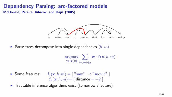
Dependency Parsing: arc-factored modelsMcDonald, Pereira, Ribarov, and Hajic (2005)
Dependency Parsing: arc-factored models
(McDonald et al. 2005)
liked today* John saw a movie that he
! Parse trees decompose into single dependencies !h, m"
argmaxy!Y(x)
!
"h,m#!y
w · f(x, h, m)
! Some features: f1(x, h, m) = [ ”saw” # ”movie” ]f2(x, h, m) = [ distance = +2 ]
! Tractable inference algorithms exist (tomorrow’s lecture)
I Parse trees decompose into single dependencies 〈h,m〉
argmaxy∈Y(x)
∑
〈h,m〉∈yw · f(x, h,m)
I Some features: f1(x, h,m) = [ ”saw” → ”movie” ]f2(x, h,m) = [ distance = +2 ]
I Tractable inference algorithms exist (tomorrow’s lecture)
68/74
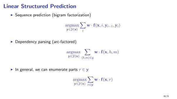
Linear Structured Prediction
I Sequence prediction (bigram factorization)
argmaxy∈Y(x)
∑
i
w · f(x, i,yi−1,yi)
I Dependency parsing (arc-factored)
argmaxy∈Y(x)
∑
〈h,m〉∈yw · f(x, h,m)
I In general, we can enumerate parts r ∈ y
argmaxy∈Y(x)
∑
r∈yw · f(x, r)
69/74
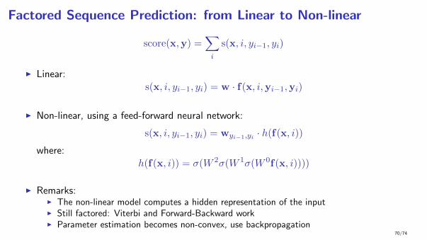
Factored Sequence Prediction: from Linear to Non-linear
score(x,y) =∑
i
s(x, i, yi−1, yi)
I Linear:s(x, i, yi−1, yi) = w · f(x, i,yi−1,yi)
I Non-linear, using a feed-forward neural network:
s(x, i, yi−1, yi) = wyi−1,yi · h(f(x, i))where:
h(f(x, i)) = σ(W 2σ(W 1σ(W 0f(x, i))))
I Remarks:I The non-linear model computes a hidden representation of the inputI Still factored: Viterbi and Forward-Backward workI Parameter estimation becomes non-convex, use backpropagation
70/74

Recurrent Sequence Prediction
. . .
x2 xnx3x1
y1 y2 y3 yn
h1 h2 h3 hn
I Maintains a state: a hidden variable that keeps track of previous observations andpredictions
I Making predictions is not tractableI In practice: greedy predictions or beam search
I Learning is non-convex
I Popular methods: RNN, LSTM, Spectral Models, . . .
71/74

Thanks!
72/74

References I
Daniel Andor, Chris Alberti, David Weiss, Aliaksei Severyn, Alessandro Presta, Kuzman Ganchev, Slav Petrov, and Michael Collins. Globally normalizedtransition-based neural networks. In Proceedings of the 54th Annual Meeting of the Association for Computational Linguistics (Volume 1: Long Papers),pages 2442–2452, Berlin, Germany, August 2016. Association for Computational Linguistics. URL http://www.aclweb.org/anthology/P16-1231.
Michael Collins. Discriminative training methods for hidden markov models: Theory and experiments with perceptron algorithms. In Proceedings of theACL-02 conference on Empirical methods in natural language processing-Volume 10, pages 1–8. Association for Computational Linguistics, 2002.
Michael Collins, Amir Globerson, Terry Koo, Xavier Carreras, and Peter L Bartlett. Exponentiated gradient algorithms for conditional random fields andmax-margin markov networks. The Journal of Machine Learning Research, 9:1775–1822, 2008.
Koby Crammer, Ryan McDonald, and Fernando Pereira. Scalable large-margin online learning for structured classification. In NIPS Workshop on LearningWith Structured Outputs, 2005.
Yoav Freund and Robert E. Schapire. Large margin classification using the perceptron algorithm. Mach. Learn., 37(3):277–296, December 1999. ISSN0885-6125. doi: 10.1023/A:1007662407062. URL http://dx.doi.org/10.1023/A:1007662407062.
Michel Galley, Jonathan Graehl, Kevin Knight, Daniel Marcu, Steve DeNeefe, Wei Wang, and Ignacio Thayer. Scalable inference and training of context-richsyntactic translation models. In Proceedings of the 21st International Conference on Computational Linguistics and the 44th annual meeting of theAssociation for Computational Linguistics, pages 961–968. Association for Computational Linguistics, 2006.
Sanjiv Kumar and Martial Hebert. Man-made structure detection in natural images using a causal multiscale random field. In 2003 IEEE Computer SocietyConference on Computer Vision and Pattern Recognition (CVPR 2003), 16-22 June 2003, Madison, WI, USA, pages 119–126, 2003. doi:10.1109/CVPR.2003.1211345. URL https://doi.org/10.1109/CVPR.2003.1211345.
John D. Lafferty, Andrew McCallum, and Fernando C. N. Pereira. Conditional random fields: Probabilistic models for segmenting and labeling sequence data.In Proceedings of the Eighteenth International Conference on Machine Learning, ICML ’01, pages 282–289, San Francisco, CA, USA, 2001. MorganKaufmann Publishers Inc. ISBN 1-55860-778-1. URL http://dl.acm.org/citation.cfm?id=645530.655813.
Yann LeCun, Leon Bottou, Yoshua Bengio, and Patrick Haffner. Gradient-based learning applied to document recognition. Proceedings of the IEEE, 86(11):2278–2324, 1998.
Andrew McCallum, Dayne Freitag, and Fernando CN Pereira. Maximum entropy markov models for information extraction and segmentation. In Icml,volume 17, pages 591–598, 2000.
73/74

References II
Ryan McDonald, Fernando Pereira, Kiril Ribarov, and Jan Hajic. Non-projective dependency parsing using spanning tree algorithms. In Proceedings of theconference on Human Language Technology and Empirical Methods in Natural Language Processing, pages 523–530. Association for ComputationalLinguistics, 2005.
Shai Shalev-Shwartz, Yoram Singer, Nathan Srebro, and Andrew Cotter. Pegasos: Primal estimated sub-gradient solver for svm. Mathematical programming,127(1):3–30, 2011.
Ben Taskar, Carlos Guestrin, and Daphne Koller. Max-margin markov networks. In Advances in neural information processing systems, volume 16, 2003.
Ioannis Tsochantaridis, Thorsten Joachims, Thomas Hofmann, and Yasemin Altun. Large margin methods for structured and interdependent output variables.Journal of machine learning research, 6(Sep):1453–1484, 2005.
74/74