learning structured probabilistic models for …ai.stanford.edu/~dvickrey/thesis.pdf · learning...
TRANSCRIPT

LEARNING STRUCTURED PROBABILISTIC MODELS FOR
SEMANTIC ROLE LABELING
A DISSERTATION
SUBMITTED TO THE DEPARTMENT OF COMPUTER SCIENCE
AND THE COMMITTEE ON GRADUATE STUDIES
OF STANFORD UNIVERSITY
IN PARTIAL FULFILLMENT OF THE REQUIREMENTS
FOR THE DEGREE OF
DOCTOR OF PHILOSOPHY
David Vickrey
June 2010

Abstract
Teaching a computer to read is one of the most interesting and important artificial
intelligence tasks. Due to the complexity of this task, many sub-problems have been
defined, mostly in the area of natural language processing (NLP). In this thesis, we
focus on semantic role labeling (SRL), one important processing step on the road
from raw text to a full semantic representation. Given an input sentence and a target
verb in that sentence, the SRL task is to label the semantic arguments, or roles, of
that verb. For example, in the sentence “Tom eats an apple,” the verb “eat” has two
roles, Eater = “Tom” and Thing Eaten = “apple”.
Most SRL systems, including the ones presented in this thesis, take as input a
syntactic analysis built by an automatic syntactic parser. SRL systems rely heavily
on path features constructed from the syntactic parse, which capture the syntactic
relationship between the target verb and the phrase being classified. However, there
are several issues with these path features. First, the path feature does not always
contain all relevant information for the SRL task. Second, the space of possible path
features is very large, resulting in very sparse features that are hard to learn.
In this thesis, we consider two ways of addressing these issues. First, we experiment
with a number of variants of the standard syntactic features for SRL. We include a
large number of syntactic features suggested by previous work, many of which are
designed to reduce sparsity of the path feature. We also suggest several new features,
most of which are designed to capture additional information about the sentence not
included in the standard path feature. We add each feature individually to a baseline
SRL model, finding that the sparsity-reducing features are not very helpful, while
iv

the information-adding features improve performance significantly. We then build an
SRL model using the best of these new and old features. This model is competitive
with state-of-the-art SRL models; in particular, when compared on features alone, it
achieves a significant improvement over previous models.
The second method we consider is a new methodology for SRL based on labeling
canonical forms. A canonical form is a representation of a verb and its arguments
that is abstracted away from the syntax of the input sentence. For example, “A
car hit Bob” and “Bob was hit by a car” have the same canonical form, {Verb =
“hit”, Deep Subject = “a car”, Deep Object = “a car”}. Labeling canonical forms
makes it much easier to generalize between sentences with different syntax. To label
canonical forms, we first need to automatically extract them given an input parse. We
develop a system based on a combination of hand-coded rules and machine learning.
This allows us to include a large amount of linguistic knowledge and also have the
robustness of a machine learning system. Since we do not have access to labeled
examples of canonical forms, we train this system directly on SRL data, treating the
correct canonical form as a hidden variable. Our system improves significantly over
a strong baseline, demonstrating the viability of this new approach to SRL.
This latter method involves learning a large, complex probabilistic model. In the
model we present, exact learning is tractable, but there are several natural extensions
to the model for which exact learning is not possible. This is quite a general issue;
in many different application domains, we would like to use probabilistic models
that cannot be learned exactly. We propose a new method for learning these kinds
of models based on contrastive objectives. The main idea is to learn by comparing
only a few possible values of the model, instead of all possible values. This method
generalizes a standard learning method, pseudo-likelihood, and is closely related to
another, contrastive divergence. Previous work has mostly focused on comparing
nearby sets of values; we focus on non-local contrastive objectives, which compare
arbitrary sets of values.
We prove several theoretical results about our model, showing that contrastive ob-
jectives attempt to enforce probability ratio constraints between the compared values.
v

Based on this insight, we suggest several methods for constructing contrastive objec-
tives, including contrastive constraint generation (CCG), a cutting-plane style algo-
rithm that iteratively builds a good contrastive objective based on finding high-scoring
values. We evaluate CCG on a machine vision task, showing that it significantly
outperforms pseudo-likelihood, contrastive divergence, as well as a state-of-the-art
max-margin cutting-plane algorithm.
vi

Acknowledgment
First I would like thank my advisor, Daphne Koller, for her help and guidance
throughout my Ph.D. I began working in Daphne’s lab as an undergraduate, so her
contribution to my academic career extends back even farther. Daphne has taught
me a huge amount about the research process, especially about presentation of work.
This ranges from rigorously exploring and testing all aspects of a model to effectively
communicating the work in papers and talks. She is also an inspiring classroom
teacher; one of the main reasons I chose to study machine learning was the classes I
took from her as an undergraduate.
I would also like to thank the other members of my reading committee, Chris
Manning and Andrew Ng. One of the best parts of studying at Stanford is the
number and quality of professors and students in the artificial intelligence lab, of
which Chris and Andrew are an essential part.
I have interacted with many other students over the years, in several groups. I have
had a number of office mates, including Pieter Abbeel, Ben Taskar, Drago Anguelov,
Suchi Saria, and Steve Gould. Suchi and Steve in particular have been a great source
for interesting discussion over the last several years. I have worked with over a
dozen Master’s and undergraduate students, many of whom made important research
contributions and were co-authors on papers. Master’s students I worked with include
Lukas Biewald, Marc Teyssier, James Connor, and Cliff Lin. The DAGS research
group has been a great source of community and research ideas, with too many names
to list. The most notable collaboration was with Varun Ganapathi and John Duchi
as part of a sizeable detour into inference in graphical models. Finally, the Stanford
vii

NLP group has been my second home at Stanford. It has been both an important
place for expanding my knowledge of natural language processing and linguistics and
another community of great students to interact with.
I would also like to thank Boeing for their support of my work, and specifically
Oscar Kipersztok at Boeing for his strong advocacy of our research group’s work and
a fruitful research collaboration. Additional thanks for financial support go to the
National Defense Science & Engineering Fellowship and the CALO project funded by
DARPA.
Finally, I would like to thank my family. My parents, Mary and Barry, and my
brother, Mark, have been a great source of support throughout my Ph.D., and earlier
they worked to provide me with the opportunities that got me here. Last but not last
is my wife, Corey, and our daughter, Matilda. I am grateful to Corey for her hard
work out in the real world while I pursued my Ph.D., but more importantly, I love
Corey as the center of my life.
viii

Contents
Abstract iv
Acknowledgment vii
1 Introduction 1
1.1 Contributions and Publications . . . . . . . . . . . . . . . . . . . . . 3
1.2 Thesis Outline . . . . . . . . . . . . . . . . . . . . . . . . . . . . . . . 5
2 Background 6
2.1 Semantic Role Labeling . . . . . . . . . . . . . . . . . . . . . . . . . . 6
2.1.1 SRL as an NLP Task . . . . . . . . . . . . . . . . . . . . . . . 7
2.1.2 Applications of SRL . . . . . . . . . . . . . . . . . . . . . . . 12
2.1.3 State-of-the-art SRL Systems . . . . . . . . . . . . . . . . . . 13
2.2 Learning Complex Probabilistic Models . . . . . . . . . . . . . . . . . 15
2.2.1 Definitions . . . . . . . . . . . . . . . . . . . . . . . . . . . . . 15
2.2.2 Using Log-linear Models . . . . . . . . . . . . . . . . . . . . . 16
3 Syntax Features for Semantic Role Labeling 20
3.1 Introduction . . . . . . . . . . . . . . . . . . . . . . . . . . . . . . . . 20
3.2 Experimental Setup . . . . . . . . . . . . . . . . . . . . . . . . . . . . 21
ix

3.3 Our Standard SRL System . . . . . . . . . . . . . . . . . . . . . . . . 21
3.4 Extended Syntactic Features . . . . . . . . . . . . . . . . . . . . . . . 25
3.4.1 Sub-paths . . . . . . . . . . . . . . . . . . . . . . . . . . . . . 25
3.4.2 Path Statistics . . . . . . . . . . . . . . . . . . . . . . . . . . 26
3.4.3 Verb Sub-categorization . . . . . . . . . . . . . . . . . . . . . 26
3.4.4 Path Modification . . . . . . . . . . . . . . . . . . . . . . . . . 27
3.4.5 Miscellaneous . . . . . . . . . . . . . . . . . . . . . . . . . . . 28
3.5 Results and Discussion . . . . . . . . . . . . . . . . . . . . . . . . . . 29
3.6 Comparison to State-of-the-art SRL Systems . . . . . . . . . . . . . . 32
4 Canonicalization for Semantic Role Labeling 35
4.1 Introduction . . . . . . . . . . . . . . . . . . . . . . . . . . . . . . . . 35
4.2 Canonical Forms . . . . . . . . . . . . . . . . . . . . . . . . . . . . . 37
4.2.1 Related Formalisms . . . . . . . . . . . . . . . . . . . . . . . . 38
4.3 Canonicalization System . . . . . . . . . . . . . . . . . . . . . . . . . 40
4.3.1 System Overview . . . . . . . . . . . . . . . . . . . . . . . . . 41
4.3.2 Transformation Rules . . . . . . . . . . . . . . . . . . . . . . . 42
4.3.3 Rule Set . . . . . . . . . . . . . . . . . . . . . . . . . . . . . . 44
4.3.4 Sequences of Rules . . . . . . . . . . . . . . . . . . . . . . . . 46
4.4 Producing Canonical Forms . . . . . . . . . . . . . . . . . . . . . . . 48
4.5 Labeling Canonical Forms . . . . . . . . . . . . . . . . . . . . . . . . 50
4.6 Probabilistic Model . . . . . . . . . . . . . . . . . . . . . . . . . . . . 51
4.7 Simplification Data Structure . . . . . . . . . . . . . . . . . . . . . . 53
4.7.1 Sharing Structure . . . . . . . . . . . . . . . . . . . . . . . . . 54
4.7.2 Rule Application . . . . . . . . . . . . . . . . . . . . . . . . . 56
4.7.3 Adding Rule Information . . . . . . . . . . . . . . . . . . . . . 59
x
4.7.4 Inference and Learning . . . . . . . . . . . . . . . . . . . . . . 60
4.8 Experiments . . . . . . . . . . . . . . . . . . . . . . . . . . . . . . . . 60
4.9 Discussion and Future Work . . . . . . . . . . . . . . . . . . . . . . . 65
5 Learning with Contrastive Objectives 67
5.1 Introduction . . . . . . . . . . . . . . . . . . . . . . . . . . . . . . . . 67
5.2 Overview . . . . . . . . . . . . . . . . . . . . . . . . . . . . . . . . . . 68
5.3 Contrastive Objectives . . . . . . . . . . . . . . . . . . . . . . . . . . 69
5.3.1 Definitions . . . . . . . . . . . . . . . . . . . . . . . . . . . . . 69
5.3.2 Relationship to Standard Learning Methods . . . . . . . . . . 70
5.3.3 Visualization of Contrastive Objectives . . . . . . . . . . . . . 71
5.3.4 Other Related Methods . . . . . . . . . . . . . . . . . . . . . 72
5.4 Theoretical Results . . . . . . . . . . . . . . . . . . . . . . . . . . . . 75
5.4.1 Consistency of Pseudo-likelihood . . . . . . . . . . . . . . . . 75
5.4.2 Finite Consistency . . . . . . . . . . . . . . . . . . . . . . . . 76
5.4.3 Asymptotic Consistency . . . . . . . . . . . . . . . . . . . . . 81
5.5 Weight Decomposition . . . . . . . . . . . . . . . . . . . . . . . . . . 83
5.6 Choosing Sub-objectives: Approximating LL . . . . . . . . . . . . . . 84
5.7 Choosing Sub-objectives: Fixed Methods . . . . . . . . . . . . . . . . 86
5.7.1 Simple Fixed Methods . . . . . . . . . . . . . . . . . . . . . . 87
5.7.2 Bias . . . . . . . . . . . . . . . . . . . . . . . . . . . . . . . . 88
5.7.3 Data-Independent Objective Example . . . . . . . . . . . . . . 90
5.8 Choosing Sub-objectives: CCG . . . . . . . . . . . . . . . . . . . . . 91
5.9 Experimental Results . . . . . . . . . . . . . . . . . . . . . . . . . . . 93
5.10 Discussion and Future Work . . . . . . . . . . . . . . . . . . . . . . . 98
6 Conclusion 100
xi

List of Tables
2.1 Phrase features for “an apple” in Figure 2.1 . . . . . . . . . . . . . . 10
3.1 Features used in our standard SRL system . . . . . . . . . . . . . . . 22
3.2 Identification classifier results . . . . . . . . . . . . . . . . . . . . . . 24
3.3 Results sequentially adding basic features . . . . . . . . . . . . . . . . . 24
3.4 Results for individually adding each feature . . . . . . . . . . . . . . 30
3.5 Results of removing features one at a time from Combo 1 . . . . . . . . . 31
3.6 Comparison to previous work on test data . . . . . . . . . . . . . . . 32
3.7 Results using reranked parses . . . . . . . . . . . . . . . . . . . . . . 33
4.1 Rule categories with sample simplifications . . . . . . . . . . . . . . . 45
4.2 F1 Measure using Charniak parses . . . . . . . . . . . . . . . . . . . . 62
4.3 F1 Measure using gold-standard parses . . . . . . . . . . . . . . . . . 62
4.4 Comparison of rule subsets . . . . . . . . . . . . . . . . . . . . . . . . 64
5.1 Pixel-wise ICM test error with standard deviation (SD) . . . . . . . . 96
5.2 Comparison of Inference Methods . . . . . . . . . . . . . . . . . . . . 98
xii

List of Figures
1.1 Parse of “Tom wants to eat an apple.” . . . . . . . . . . . . . . . . . . 2
1.2 Path features for verb “eat” in Figure 1.1 . . . . . . . . . . . . . . . . . 2
2.1 Parse of “Tom wants to eat an apple.” . . . . . . . . . . . . . . . . . . 8
2.2 Path features for verb “eat” . . . . . . . . . . . . . . . . . . . . . . . 10
2.3 CRF for classifying regions in an image . . . . . . . . . . . . . . . . . 16
3.1 Parse with example path features for verb “eat” . . . . . . . . . . . . . 23
4.1 Canonical forms for all verbs in “Tom wants to eat an apple.” . . . . . . 36
4.2 Example tree pattern and matching constituents . . . . . . . . . . . 42
4.3 Result of applying add-child-end(3,2) in Figure 4.2 . . . . . . . . . . 42
4.4 Rule for depassivizing a sentence . . . . . . . . . . . . . . . . . . . . 44
4.5 Iterative transformation rule application . . . . . . . . . . . . . . . . . 47
4.6 Histogram of canonical form/rule set pairs . . . . . . . . . . . . . . . 49
4.7 Histogram of canonical form/rule set/labeling triples . . . . . . . . . 49
4.8 Features for example canonical form . . . . . . . . . . . . . . . . . . . 52
4.9 Separate parses for “I will go” and “I go” . . . . . . . . . . . . . . . 54
4.10 Using a choice node to share structure . . . . . . . . . . . . . . . . . 55
4.11 Sharing structure using a directed acyclic graph . . . . . . . . . . . . 55
xiii

4.12 F1 Measure on WSJ test set as a function of training set size . . . . . 63
5.1 Probability distribution and observed data set . . . . . . . . . . . . . 72
5.2 Visualization of log-likelihood gradient . . . . . . . . . . . . . . . . . 72
5.3 Visualization of pseudo-likelihood . . . . . . . . . . . . . . . . . . . . 73
5.4 Visualization of local pairwise sub-objective . . . . . . . . . . . . . . 73
5.5 Visualization of non-local pairwise sub-objective . . . . . . . . . . . . 73
5.6 Visualization of “satisfied” pairwise sub-objective . . . . . . . . . . . 73
5.7 Parameter estimation for different contrastive objectives . . . . . . . 87
5.8 Original image and correct region labeling . . . . . . . . . . . . . . . . 93
5.9 Pixel-wise ICM test error . . . . . . . . . . . . . . . . . . . . . . . . . 96
5.10 Test Error vs. Running Time (in seconds) . . . . . . . . . . . . . . . 97
xiv

Chapter 1
Introduction
Teaching a computer to read is one of the most interesting and challenging problems
in computer science. The field of natural language processing (NLP) developed as
a response to the difficulty of this problem. One of the important developments in
NLP has been the introduction and study of a number of sub-problems that break
the task down into a number of more manageable sub-tasks. In this thesis, we focus
on one of these tasks, semantic role labeling (SRL), an important processing step on
the road from raw text to a full semantic representation.
Given an input sentence and a target verb in that sentence, the SRL task is to label
the semantic arguments, or roles, of that verb. For example, in the sentence “Tom
eats an apple,” the verb “eat” has two roles, Eater = “Tom” and Thing Eaten =
“apple”. This task lies somewhere in the middle between syntax and semantics: it is
more semantic than tasks such as part of speech tagging or syntactic parsing, but less
semantic than tasks such as information extraction or question answering. Previous
work, e.g., (Shen & Lapata, 2007; Christensen et al., 2010), have shown that using
the output of an SRL system improves performance for a variety of these higher-level
tasks.
Most semantic role labeling systems, including the ones presented in this thesis, take
as input a syntactic analysis built by an automatic syntactic parser. SRL systems rely
heavily on features extracted from the syntactic parse, particularly the path feature
1

CHAPTER 1. INTRODUCTION 2
TO
S NP VP
Tom VBD
NN eat
wants VP
an DT
VB to
NNP S
NP
apple
VP
Figure 1.1: Parse of “Tom wants to eat an apple.”
NP S VP Tom: S VP VP T
an apple: VP T NP
Figure 1.2: Path features for verb “eat” in Figure 1.1
(Gildea & Jurafsky, 2002), which captures the syntactic relationship between the
target verb and the phrase being classified. Figures 1.1 and 1.2 show the parse and
path features for several phrases in a sample sentence. The parse and the path feature
are explained in more detail in Chapter 2.
Unfortunately, there are several issues with path features. First, the path feature
may not contain all relevant information for the SRL task. Second, the space of
possible path features is very large, resulting in very sparse features that are hard to
learn.
In this thesis, we consider two ways of addressing these issues. First, we experiment
with a number of variants of the standard syntactic features for SRL. We include a
large number of syntactic features suggested by previous work, many of which are
designed to reduce the sparsity of the path feature. We also suggest several new

CHAPTER 1. INTRODUCTION 3
features, most of which are designed to capture additional information about the
sentence not included in the standard path feature.
The second method we consider is a new methodology for SRL based on labeling
canonical forms. A canonical form is a representation of a verb and its arguments
that is abstracted away from the syntax of the input sentence. For example, “A
car hit Bob,” and “Bob was hit by a car,” have the same canonical form, {Verb =
“hit”, Deep Subject = “a car”, Deep Object = “a car”}. Labeling canonical forms
makes it much easier to generalize between sentences with different syntax. To label
canonical forms, we first need to automatically extract them given an input parse. We
develop a system based on a combination of hand-coded rules and machine learning.
This allows us to include a large amount of linguistic knowledge and also have the
robustness of a machine learning system.
This latter method involves learning a large, complex probabilistic model. Our
model is structured in such a way that exact learning is tractable. However, there
are several natural extensions to the model for which exact learning is not possible.
This issue is not restricted to our problem; in many different application domains, we
would like to use probabilistic models that cannot be learned exactly.
We propose a new method for learning these kinds of models based on contrastive
objectives. The main idea is to learn by comparing only a few possible values of the
model, instead of all possible values. This method generalizes a standard learning
method, pseudo-likelihood, and is closely related to another, contrastive divergence.
Previous work has mostly focused on comparing nearby sets of values; we focus on
non-local contrastive objectives, which compare arbitrary sets of values. As we will
see, using non-local contrastive terms results in significant performance gains.
1.1 Contributions and Publications
There are three main contributions of this thesis:

CHAPTER 1. INTRODUCTION 4
1. Building an improved set of syntactic features for semantic role label-
ing. While there has been some previous work, e.g., (Pradhan et al., 2005), on
evaluating individual features for SRL, this thesis presents the most comprehen-
sive study of syntactic features. Additionally, we suggest several features that
incorporate additional information into the SRL system, leading to significant
gains in performance.
2. Developing a new method for semantic role labeling using canonical
forms. This system performs a much more detailed analysis of the input parse
than standard SRL systems. Normalizing sentences to a common form allows
significantly improved generalization between different sentences. Efficient im-
plementation of this system involved development and use of sophisticated al-
gorithms and data structures, as well as encoding of a large amount of linguis-
tic knowledge. This system improves significantly over a standard (but high-
performing) SRL system. This work has appeared in (Vickrey & Koller, 2008b)
and a follow-up paper, (Vickrey & Koller, 2008a).
3. Proposing non-local contrastive objectives as a means to learn complex
probabilistic models. Contrastive objectives have been described in various
forms in previous work, e.g., (LeCun & Huang, 2005; Smith & Eisner, 2005), but
this work focuses on local terms. Non-local methods have been suggested in the
context of max-margin methods (Tsochantaridis et al., 2005), but our method is
the first application of this idea to log-linear models, which, unlike margin-based
models, are able to model probability distributions. We prove several theoretical
results that justify the use of non-local contrastive objectives. One implication
of these results is that contrastive objectives attempt to enforce probabilistic
ratio constraints between compared values. Based on this insight, we propose
contrastive constraint generation (CCG), which uses MAP inference to find values
to include in our contrastive objective. Experimental results on a real-world
machine vision task show that CCG improves significantly over local contrastive
learning methods such as pseudo-likelihood and contrastive divergence, as well
as the margin-based method of Tsochantaridis et al. (2005). This work has been

CHAPTER 1. INTRODUCTION 5
accepted for publication as (Vickrey et al., 2010).
1.2 Thesis Outline
Chapter 2: Background. This chapter introduces the necessary background for
semantic role labeling and for learning complex probabilistic models. This chapter
also includes an overview of previous work in semantic role labeling and a few basic
citations in the area of probabilistic learning. More specific related work is included
in each of the subsequent chapters.
Chapter 3: Evaluating Syntactic Features for Semantic Role Labeling.
In this chapter, we first describe the details of our implementation of a standard SRL
system. Next, we describe a number of additional syntactic features, both new and
old. We then do a detailed experimental evaluation on these features and build a
final model using the best features. Finally, we compare our model to several state-
of-the-art SRL models on the standard CoNLL test set.
Chapter 4: Canonicalization for Semantic Role Labeling. In this chapter,
we first present the idea of a canonical form. We then describe how we build an SRL
system based on labeling canonical forms. We describe the linguistic knowledge that
went into building the system, as well as the data structures and algorithms that
allowed us to learn and perform inference in our model. Finally, we evaluate our
model on the CoNLL test set and compare it to our standard SRL system.
Chapter 5: Non-Local Contrastive Objectives. In this chapter, we begin by
defining contrastive objectives and discussing their relationship to several well-known
learning methods. Next, we present several theoretical results, including consistency
of contrastive objectives with maximum likelihood. We then propose several methods
for constructing contrastive objectives, including contrastive constraint generation
(CCG). Finally, we evaluate CCG on a machine vision task, comparing it to several
well-known learning methods.

Chapter 2
Background
We first describe background material for semantic role labeling, followed by a dis-
cussion of learning complex probabilistic models.
2.1 Semantic Role Labeling
The first three chapters of this thesis focus on the task of semantic role labeling (SRL).
A single instance of this problem is a sentence and a target verb within that sentence.
The goal is to label the semantic arguments, or roles, of that verb. For example, in
the sentence “Tom eats an apple,” the verb “eat” has two roles, Eater=“Tom” and
Thing Eaten=“apple”. Roles are not the same as syntactic arguments (e.g., subject,
direct object), although certain semantic arguments often coincide with syntactic
arguments. For example, the subject of “eat” is usually the Eater, but in many
sentences the Eater is not the syntactic subject of “eat” (e.g., in “Tom wanted to eat
an apple”, “Tom” is the subject of “want”, not “eat”). For other verbs, the syntactic
subject may take several possible roles. In “Tom sold the house,” the syntactic subject
“Tom” is the Seller, but in “The house sold,” the syntactic subject “house” is the
Thing Sold.
In this thesis, we focus on the PropBank (Kingsbury et al., 2002) data set and its
associated role set. Other notable data sets for SRL (not discussed in this thesis) are
6

CHAPTER 2. BACKGROUND 7
FrameNet (Baker & Sato, 2003)1 and VerbNet (Schuler, 2006)2. These data sets are
similar to PropBank but have some important differences.
PropBank contains a single set of roles which are used across all annotated verbs.
These roles are divided into two types. The first type, core arguments, consists of verb-
specific roles, labeled ARG0 through ARG5. ARG0 is generally the agent, ARG1 is
generally the theme, while ARG2-ARG5 have different usages for verbs. For example,
for “eat”, ARG0 corresponds to the Eater, and ARG1 is the Thing Eaten. For “give”,
ARG0 is the Giver, ARG1 is the Gift, and ARG2 is the Recipient. The second type,
adjunct arguments, corresponds to arguments that are not specific to particular verbs.
Examples include time phrases (labeled ARGM-TMP) and location phrases (labeled
ARGM-LOC). There are twelve different types of adjunct arguments.
Throughout the thesis, we use the ARGX labels for specific roles, but we often
include in parentheses the verb-specific interpretation of that argument. For example,
if we are talking about the ARG0 of “eat”, we write ARG0(Eater).
2.1.1 SRL as an NLP Task
Semantic role labeling has a long history in linguistics and natural language process-
ing (NLP). We will not discuss the earlier work in this thesis; Pradhan (2006), for
example, gives a good overview. Semantic role labeling was reintroduced in a modern
machine learning setting by Gildea & Jurafsky (2002). The standard approach to this
problem is to build a classifier based on a large number of features extracted from a
syntactic analysis of the sentence. In this section we will describe the basic setup of
the problem and standard features used for this task.
Automatic syntactic parsers, such as the Charniak parser3, play an essential role
in most SRL systems. Until recently, most work was based on constituency parsers,
such as the Charniak parser; in the last few years there has been a significant amount
of work using dependency parsers for SRL. Johansson & Nugues (2008) built an early
1http://framenet.icsi.berkeley.edu2http://verbs.colorado.edu/∼mpalmer/projects/verbnet.html3Available at ftp://ftp.cs.brown.edu/pub/nlparser/

CHAPTER 2. BACKGROUND 8
TO
S NP VP
Tom VBD
NN eat
wants VP
an DT
VB to
NNP S
NP
apple
VP
Figure 2.1: Parse of “Tom wants to eat an apple.”
dependency-based SRL system, while the CoNLL 2008 shared task4 focused on joint
dependency parsing/SRL. Both types of parsers work well for SRL; the best systems
using each type of parser achieve roughly comparable results. Since the different
types of parse require different feature extractors, it is generally easier to choose one
type and concentrate on it, particularly for more complicated methods such as the
one presented in Chapter 4. In this thesis, we exclusively use constituency parses.
Figure 2.1 shows an example constituency parse. A constituency parse is a rooted
tree where each node is labeled with a category. For example, the root of the tree in
Figure 2.1 is labeled with category S, indicating that it is a sentence or sentence clause.
The first child of this node is labeled with category NP, indicating a noun phrase. The
leaves of the tree are labeled with the words of the sentence; the immediate parent
of each leaf is labeled with that word’s part of speech tag. A constituent refers to a
complete subtree of the parse. Example constituents in Figure 2.1 include “Tom,”
“an apple,” and “wants to eat an apple.” The type of a constituent is the category
of the root of the constituent subtree.
4Available at http://barcelona.research.yahoo.net/conll2008/

CHAPTER 2. BACKGROUND 9
Problem Definition
Given a syntactic parse, standard SRL systems solve the following problem. For
every sentence s, for every verb v in s, for every constituent c in the parse of s, the
system must decide whether c is an argument of v, and if so, which of the possible
roles it should be labeled with. Let R be the set of all possible roles (both core and
adjuncts), plus one additional value “none.” Each triple s, v, c is considered to be a
separate training example and is labeled with a role r ∈ R: if c is an argument of v, r
is the correct role of c; otherwise r = “none.” The data set D contains m examples;
example di corresponds to the triple (si, vi, ci), with label ri ∈ R. Note that none of
si, vi, ci is unique to di; each may occur in multiple different examples.
Given this setup, we now have a straightforward (multi-class) classification problem
and can use any of a variety of standard classifiers, such as logistic regression or SVM.
A large amount of effort has been made in previous work to determine useful features
for this task. Later in this section, we will discuss several “basic” features that are
used by most high-performing systems; in Chapter 3 we will describe a number of
other features that have been proposed for SRL.
Parse-related Complications
The use of automatically-generated parses introduces a complication: the correct
argument phrases may not line up with a single constituent in the automatic parse. In
principle, the system can recover, since any group of words from the original sentence
can be covered by some set of constituents. However, this is quite difficult for the
SRL classifier, so typically the system will end up with an incorrect role labeling if
this happens (incorrect with respect to the most commonly used scoring metrics).
Another issue is how to deal with overlapping predictions by the role classifier.
For example, suppose the role classifier decides to label a particular constituent as
ARG0, but decides to label one of its children as ARG1. One simple solution to this
problem is to use greedy top-down decoding, where the role assigned to a constituent
is propagated (and overwrites) any labelings of its descendants. More complicated

CHAPTER 2. BACKGROUND 10
Feature Example CitationFrame eat (Gildea & Jurafsky, 2002)Head Word apple (Gildea & Jurafsky, 2002)Category NP (Gildea & Jurafsky, 2002)Head POS NN (Surdeanu et al., 2003)First Word an (Pradhan et al., 2005)Last Word apple (Pradhan et al., 2005)
Table 2.1: Phrase features for “an apple” in Figure 2.1
NP S VP Tom: S VP VP T
an apple: VP T NP
Figure 2.2: Path features for verb “eat” in Figure 2.1. T represents the target verb.
methods have been proposed, see for example (Toutanova et al., 2005). The choice
of method used to solve this problem can also influence the method used to train the
system; we return to this issue in the next chapter.
Basic Features
There are two basic categories of SRL features. The first is features of the constituent,
which we refer to as phrase features. Table 2.1 lists the most commonly-used (and suc-
cessful) phrase features for SRL. Head words are typically computed using a heuristic
head-word system, as in the head rules of Collins (1999). These features allow us to
capture syntactic and lexical patters. For example, we can learn that “apple” is likely
to be the ARG1 (Thing Eaten), but not the ARG0 (Eater).
The most important syntactic feature in most SRL systems is the path of category
nodes from the constituent to be classified c to the target verb v (Gildea & Jurafsky,
2002). Examples of this feature are shown in Figure 2.2.5 Path features allow systems
5There are several decisions to make when constructing the path feature, such as whether to usea directed or undirected path. Shown is the version of this feature we use in our models, describedin more detail in Chapter 3.

CHAPTER 2. BACKGROUND 11
to capture both general patterns, e.g., that the ARG0 of a sentence tends to be the
subject of the sentence, and specific usage, e.g., that the ARG2 (Recipient) of “give”
is often a post-verbal prepositional phrase headed by “to”. Another commonly-used
syntactic feature is the length (number of edges) in the path feature (Pradhan et al.,
2005).
The final basic syntactic feature we discuss is the sub-categorization of the target
verb (Gildea & Jurafsky, 2002). This feature is simply the CFG expansion of the par-
ent of the target verb. In Figure 2.1, the sub-categorization for “eat” is V P→T NP .
As described above, many of the roles (ARG0, ARG1, and the adjuncts) behave
similarly across different verbs. To take advantage of this, we can include both a
general and a frame-specific version of each feature. Consider the Head Word feature
(described below). In Figure 2.1, for verb “eat” and constituent “an apple”, we can
extract both the general feature “head-word=apple” and the frame-specific feature
“frame=eat,head-word=apple.” Frame-specific versions of the head word, path, and
category features are often used, as suggested by Xue & Palmer (2004), but frame-
specific versions of the other feature types are less common.
Identification Classifier
There is one practical problem with the system described so far. The PropBank
training set is fairly large (one million words), and in the setup described, for every
verb v in every sentence s, we label every constituent c in the parse of s. This leads to
a very large training set, which is made worse by the fact that training time typically
scales linearly with the number of classes (in this case, the number of roles |R| ≈ 30).
To address this issue, many systems introduce an additional preprocessing step in
order to filter out constituents that are “clearly” not arguments. This is usually just
a binary classifier that uses similar features to those used by the role classifier, which
is supposed to answer 1 if the constituent is an argument, and −1 otherwise. This
identification classifier is trained on the same training set as the classifier, and is then

CHAPTER 2. BACKGROUND 12
used (at both training and test time) to reduce the set of constituents that are pro-
cessed by the role classifier.6 Often, the classification threshold for the identification
classifier is set to increase recall at the cost of precision. Since constituents that are
not actually arguments can make it through the filtering stage, the role classifier still
needs the option to classify a constituent as “none.”
2.1.2 Applications of SRL
SRL is a natural pre-processing step for tasks such as information extraction and
information retrieval. For example, a typical information extraction task is to find all
events of a certain type (e.g., one company buying another), along with who bought
whom, when, for what price, etc. Since many such events appear in text as verbs
with their associated semantic roles, it is clearly useful to be able to identify these
roles automatically. More generally, SRL is an important step for any system that
aims to achieve “natural language understanding.”
Following is a list of applications of SRL to higher-level tasks:
Christensen et al. (2010) build a system based on SRL for open-domain information
extraction (Open IE) — the task of extracting factual relationships from a text corpus
without using a prespecified list of relations. Their SRL-based system obtains higher-
quality extractions as compared to a state-of-the-art Open IE system.
Ponzetto & Strube (2006) use SRL as part of system that performs coreference
resolution — determining when two or more phrases refer to the same real-world
object. They directly use the output of a SRL system as features for their model, and
show that adding these features significantly improves performance over a baseline
model.
Shen & Lapata (2007) build a question-answering system which incorporates SRL
data from the FrameNet data set. The resulting system performs significantly better
than a system which uses only syntactic information.
6Ideally, we train the identification classifier in several folds of the training data, so that we donot end up with an overly confident filter on the training set.

CHAPTER 2. BACKGROUND 13
Kim & Hovy (2006) build an opinion mining system which uses an SRL system to
identify the opinion holder and opinion text.
Barnickel et al. (2009) build a large-scale automatic relation extraction system for
biomedical texts whose most important component is an SRL system.
Taking a step back from individual applications, the overall pattern is that SRL
systems improve performance because they perform a more-detailed analysis of the
syntax and word-level semantics of the input sentence. In principle (and sometimes
in practice), higher level tasks can directly incorporate these kinds of features, by-
passing the need for a separate SRL system.
With this in mind, the study of SRL as a separate task is important for several
reasons. First, SRL systems are a useful off-the-shelf tool which free users from
reinventing these kind of detailed features and models. Second, studying SRL as a
stand-alone task gives more insight into new features which may improve performance,
of both SRL and higher-level systems. In this respect, SRL systems are similar to
POS taggers, named entity recognizers, or syntactic parsers; much of the business of
NLP is commoditizing these sub-tasks for use by higher-level systems.
2.1.3 State-of-the-art SRL Systems
There are at least four different ways in which prior work has extended the basic
model. The first is to use additional features; in the following chapter we will go
into detail about a wide variety of features that have been proposed for SRL. In this
section, we describe three other approaches, each utilized by a different state-of-the-
art SRL system.
Punyakanok et al. (2005) built the system that placed first in the CoNLL-2005
evaluation. They start with a basic SRL system as described in this chapter. They
improve their system by running their classifier on not just on the top-scoring Char-
niak parse, but also on the next four highest-scoring Charniak parses and the highest
scoring parse generated by the Collins parser (Collins, 1999). Their system then
votes on the final role predictions by combining the predictions of the classifier run
CHAPTER 2. BACKGROUND 14
on each of these six parses. This results in a very large boost in performance, which
explains their system’s top finish. The next three systems at CoNLL-2005 also used
information from more than one parse.
Toutanova et al. (2008) looked at using joint inference for SRL. The idea is to
model the interaction between different arguments of a verb in order to improve
performance. Most obviously, most arguments can only appear once for a particular
verb (there cannot be two Agents, for example). Other more complicated patterns
can occur; for example, if there is a Recipient in the sentence, there is probably also
a Gift. Toutanova et al. (2008) incorporate this information by using a reranking
system, which first generates plausible labelings of all phrases in the sentence using
a local classifier, and then picks among those by using more global features.
Surdeanu et al. (2007) describe the system that currently has the best reported
results for SRL on the CoNLL-2005 data set. They start by building three different
syntactic SRL systems. The first two models (M1 & M2) operate quite differently
from the approach described in this chapter: they label the roles using sequence
tagging techniques similar to those commonly used for named entity extraction and
other similar tasks. Their B-I-O (beginning-inside-outside) system first uses a syn-
tactic processor (a shallow parser for M1 and the Charniak parser for M2) to build
syntactic features of each phrase. It then does linear decoding to find the optimal role
assignment. The M3 system has the same setup as the basic system we describe in
this chapter, classifying the constituents generated by the Charniak parser. The key
idea of their work is to combine these three systems to get the final role predictions;
see Surdeanu et al. (2007) for details of the combination scheme.
In this thesis, we pursue yet another direction. Our goal is to build a more so-
phisticated, “deeper” model of sentence syntax. We design features which capture
additional information about various syntactic constructs (Chapter 3), and we de-
sign a system (Chapter 4) which not only captures this kind of information but also
models the recursive structure of natural language.
CHAPTER 2. BACKGROUND 15
2.2 Learning Complex Probabilistic Models
2.2.1 Definitions
A log-linear model specifies a conditional probability distribution over a set of n label
variables Y = {Y1, . . . , Yn} given a (possibly empty) set of observed variables X. The
model space PΘ is determined by a set of R feature functions f1(X,Y), . . . , fR(X,Y);
let f(X,Y) be a vector containing all feature functions. A particular model Pθ is
defined by a vector of weights θ ∈ Θ of length R. The probability distribution
associated with Pθ is
Pθ(Y = y|X = x) =eθT f(x,y)
Z(x),
where Z(X = x) =∑
y eθT f(x,y) is a normalization factor that ensures that the
distribution sums to 1 for each x.
One of the simplest examples of a log-linear model is logistic regression, where Y
is a single variable to be predicted based on the input features X. In this thesis, we
focus on more complex models where Y consists of multiple variables. These types
of models are commonly referred to as undirected graphical models, particularly when
the connections between the label variables Yl (as specified by the feature functions)
only involve a few variables at a time. In this case, it is natural to think of the feature
functions as corresponding to edges in a graph. This is particularly natural for pair-
wise undirected graphical models, where each feature function depends on at most two
variables. Thus, each feature function depends either on only one variable (a singleton
feature) or on two variables Yl1 , Yl2 , in which case we say there is an edge between Yl1
and Yl2 . Undirected graphical models are often referred to as Markov random fields
(MRFs) when x is empty, and as conditional random fields (CRFs) (Lafferty et al.,
2001) when x is nonempty.
Undirected graphical models allow complicated probabilistic models to be specified
using relatively few parameters. This is advantageous not only computationally, but
also because it enables the model to generalize better to unseen data. Undirected
graphical models are used in a wide-range of applications, including natural language
CHAPTER 2. BACKGROUND 16
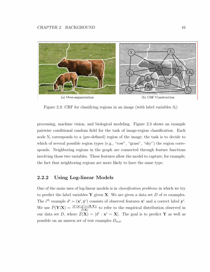
Figure 2.3: CRF for classifying regions in an image (with label variables Sl)
processing, machine vision, and biological modeling. Figure 2.3 shows an example
pairwise conditional random field for the task of image-region classification. Each
node Yl corresponds to a (pre-defined) region of the image; the task is to decide to
which of several possible region types (e.g., “cow”, “grass”, “sky”) the region corre-
sponds. Neighboring regions in the graph are connected through feature functions
involving those two variables. These features allow the model to capture, for example,
the fact that neighboring regions are more likely to have the same type.
2.2.2 Using Log-linear Models
One of the main uses of log-linear models is in classification problems in which we try
to predict the label variables Y given X. We are given a data set D of m examples.
The ith example di = (xi,yi) consists of observed features xi and a correct label yi.
We use P (Y|X) = |di:(xi,yi)=(X,Y)|Z(X)
to refer to the empirical distribution observed in
our data set D, where Z(X) = |di : xi = X|. The goal is to predict Y as well as
possible on an unseen set of test examples Dtest.

CHAPTER 2. BACKGROUND 17
Learning
The first task we need to solve is the learning problem: how to choose a good model
Pθ from our model space PΘ. A common approach is to define an objective function
over θ, and then optimize this objective to find a good choice of θ. The canonical
example of this approach for a log-linear model is the log-likelihood objective,
LL(θ; D) =∑
(xi,yi)
log Pθ(yi|xi).
This objective simply measures the average (log) probability assigned by the model Pθ
to the data examples di. This objective is concave in θ, and so as long as computing
Pθ(yi|xi) is feasible, it is straightforward to optimize this objective using standard
convex-optimization methods such as conjugate gradient or L-BFGS (Liu & Nocedal,
1989).
Unfortunately, for many log-linear models over complex label spaces, the computa-
tion of the normalization factor Z(X) — referred to as the partition function in the
context of undirected graphical models — is not feasible. For example, in an undi-
rected graphical model, the size of the label space Y is exponential in the number of
variables Yl. In certain cases, dynamic programming can be used to compute this sum
over exponentially many values, but often exact computation of Z(X) is not possible.
There are many approaches to this problem. One common method is to use approx-
imate marginal inference algorithms to compute the statistics necessary for learning.
We will not describe this approach in detail, but we briefly discuss approximate in-
ference algorithms below. Examples of this approach include sampling methods (e.g.,
Markov chain Monte Carlo sampling) and message passing algorithms (e.g., belief
propagation). Another common method, which we adopt in Chapter 5, is to de-
sign an alternate objective function that is easier to optimize but still prefers “good”
models Pθ.
One well-known example of this latter approach is pseudo-likelihood (PL). Let
dom(Yl) denote the set of possible values of Yl. Let y−l be the value of all nodes
except node l, and (y−l, yl) be a combined instantiation to y which matches yl for

CHAPTER 2. BACKGROUND 18
node l and y−l for all other nodes. The pseudo-likelihood objective is defined as
PL(θ; D) =∑
(xi,yi)
∑l
(θT f(xi,yi)− log
∑a∈dom(Yl)
eθT f(xi,(yi−l,a))
).
We will explain the motivation for this objective in more detail in following sections.
For now, there are two important properties of this objective. First, under certain
conditions, it is consistent with log-likelihood — that is, given an infinite amount of
training data, it will learn the same parameter θ as log-likelihood. Second, the time
required to compute PL(θ; D) is linear in the size of the training data; unlike log-
likelihood, it does not scale exponentially with the number of network variables. This
means that optimizing this objective is guaranteed to be computationally efficient.
Another type of alternate objective is max-margin objectives, including single-
variable models, such as support vector machines (Cortes & Vapnik, 1995; Vapnik,
1998), and complex structured models (Taskar et al., 2003; Tsochantaridis et al.,
2005). Rather than fit a probability distribution to the observed data, these methods
try to enforce constraints on the (unnormalized) score function θT f(xi,yi). As a re-
sult, computation of the partition function is not required; the model can be learned
using only MAP inference (described below). However, exact optimization of these
objectives is still intractable when MAP inference is intractable.
Inference
Once we have selected (learned) a model Pθ, we still need to actually use the model
to make predictions. This typically means that given a set of features x, we need
to find the value of Y which maximizes Pθ(Y|x). This is known as the maximum
a-posteriori (MAP) inference problem. This problem does not require computation of
the partition function Z(x) because it only requires comparison of the unnormalized
scores θT f(x,y).
There are some models for which computing Z(x) is not feasible, but computing
arg maxY Pθ(Y|x) is. MAP inference based on graph cuts is one important exam-
ple of this (see, for example, (Kolmogorov & Zabih, 2004)). For example, suppose

CHAPTER 2. BACKGROUND 19
we want to assign each pixel in an image to either “foreground” or “background”.
We allow arbitrary single-node potentials, but our model is restricted to be asso-
ciative — the weights on the pairwise features must encourage neighboring pixels
to match. Under these conditions, we can find the optimal assignment of pixels to
foreground/background by constructing a special graph and then running a max-flow
algorithm to find the minimum cut.
Unfortunately, in many cases where computing Z(x) is not feasible, computing
arg maxY Pθ(Y|x) is also not feasible. The solution to this problem is to use an
approximate MAP inference algorithm. These methods try to find a value of Y with
a high score but are not guaranteed to find the best possible value. One example of an
approximate MAP inference algorithm is iterated conditional modes (ICM), proposed
by Besag (1986). ICM is a simple greedy ascent algorithm. At each round, a variable
is chosen at random; the label of this variable is then changed to the value that gives
the highest score (if the current value is the best, the label is not changed). This
is repeated until a local maximum is reached (i.e., no single-variable moves improve
the score). Another commonly-used approximate MAP inference algorithm is max-
product belief propagation (MP) (Pearl, 1988). The details of this method are not
important for exposition of our work, but intuitively this method iteratively updates
a set of “beliefs,” one per variable, about what the best value of that variable is.
A significant advantage of MAP inference vs. marginal inference is that the MAP
inference problem is just a standard combinatorial optimization problem, which has
been well studied in a variety of computer-science fields. This is one of the primary
motivations for the methods presented in Chapter 5: they enable us to learn a log-
linear model using a MAP inference method rather than a marginal inference method.

Chapter 3
Evaluating Syntactic Features for
Semantic Role Labeling
3.1 Introduction
In this chapter, we first describe our implementation of a high-performing standard
SRL system. Second, we survey previous work in order to collect a long list of
syntactic features proposed for SRL. Third, we propose several new features, many of
which are based on incorporating additional information about specific grammatical
constructs. Fourth, we systematically evaluate the relative usefulness of both the old
and new features. Fifth, based on these experiments, we add the best-performing
features (a mix of old and new features) to our standard SRL system, improving
performance significantly. Finally, we compare to current state-of-the-art methods
for SRL. While a few systems out-perform the system we describe in this chapter,
our system has the best reported results among systems that classify each argument
independently (non-jointly) and that use information from only a single automatic
parse.
20

CHAPTER 3. SYNTAX FEATURES FOR SEMANTIC ROLE LABELING 21
3.2 Experimental Setup
Throughout this chapter, we will present results for various SRL systems on the
PropBank data set. To facilitate comparison with other work, we use the experimental
setup of the CoNLL 2005 SRL task1. Following standard procedure, we use sections
2-21 as the training set, section 24 as the development set, and section 23 as the
test set. The training set contains approximately 1 million words of text annotated
with semantic role labels. All results we report are computed using the srl-eval script
distributed by the CoNLL 2005 shared task.
As discussed in the previous chapter, an important element of most SRL systems
is an automatic syntactic parser. In this work, we use the Charniak parser Charniak
(2000), a state-of-the-art constituency parser. As noted by Toutanova et al. (2008),
the Charniak parses distributed with CoNLL 2005 did not handle forward quotes
correctly; for all the systems discussed in this thesis, we reparsed the training and
test sets using the 2005 version of the Charniak parser.2
Throughout the rest of this chapter, we report results of various versions of our
system on the training set (using 3-fold cross validation) and on the development
set. To avoid implicitly overfitting the test set, we only report test results for a few
specific feature sets, chosen based on development and training performance, not on
test performance. We did not directly compute statistical significance intervals for
our results, but we note that on the CoNLL 2005 test set, using bootstrap resampling,
all submitted systems were assigned a significance interval of ±0.8 or less F1 points.
We would expect a much smaller confidence interval on the much larger training set.
3.3 Our Standard SRL System
In this section we describe the details of our implementation of the standard SRL
system discussed in the previous chapter.
1http://www.lsi.upc.es/∼srlconll/home.html2Available at ftp://ftp.cs.brown.edu/pub/nlparser/

CHAPTER 3. SYNTAX FEATURES FOR SEMANTIC ROLE LABELING 22
Phrase Features Syntactic FeaturesFrame PathHead Word Path LengthCategory Verb SubcategorizationHead POSFirst WordLast Word
Table 3.1: Features used in our standard SRL system
Our system is based on multi-class logistic regression. From each data example di,
we extract a feature vector f i of length K. For each possible role r ∈ R, our model
has a parameter vector θr of length K. The model assigns probabilities P (r|s, v, c) =eθT
r fiPr′ e
θTr′
fi . We train the system by maximizing the L2-regularized log-likelihood,
(∑di
log P (ri|si, vi, ci)
)−∑
r
θTr θr
2σ2.
L2-regularization penalizes large weights, helping to prevent overfitting. For all results
in this chapter, we use σ = 1.0; this value gave good performance on the development
set for a wide variety of feature sets. It is possible that better performance might be
achieved by fitting σ (on the development set) separately for each feature set. We
maximize the objective using L-BFGS (Liu & Nocedal, 1989).
We use the same basic features described in Chapter 2. We prune any features that
occur fewer than 3 times in the training set. Table 3.1 is a complete list of the features
used by our basic system (refer to Chapter 2 for a description of these features). We
now describe some specific details of our implementation of these features.
To generate the Head Word and Head POS features, we use the head-word rules
of Collins (1999). As suggested by Surdeanu et al. (2003), rather than using the
preposition as the head word of prepositional phrases (PPs), we instead use the head
word of the object of the phrase. Also, we augment the category of all PPs with the
preposition. Thus, in the sentence “I gave the ball to him,” the head word of the
phrase “to him” is “him,” while the category of this phrase is “PP(to).”

CHAPTER 3. SYNTAX FEATURES FOR SEMANTIC ROLE LABELING 23
TO
S NP VP
Tom VBD
NN eat
wants VP
the DT
VB to
NNP S
NP
park
NP S VP Tom:
VP
S VP VP T the park: VP T NP
PP IN at
PP(at)
Figure 3.1: Parse with example path features for verb “eat”
There are several choices to be made regarding the path feature. In this thesis,
we use directed paths (as opposed to undirected paths); we replace the category of
the target verb v with “T” to make the paths tense-independent; and as above, we
augment prepositional phrase categories with the head preposition. Examples of our
version of the path feature are shown in Figure 3.1.
For the basic version of the subcategorization feature, we do not expand the cat-
egories of “PP” phrases — we consider this variant in the subsequent section. Note
that in some cases, the v is not actually the head of a VP phrase; in our system, we
calculate the subcategorization feature even in these cases.
In the previous chapter, we mentioned that it is important to include both frame-
specific and general versions of each feature. Most systems include general versions of
all features, but only include frame-specific versions of a few features (e.g. Head Word,
Path, and Category). We found that using frame-specific versions of other features
worked well, and so for all experiments, we include both general and frame-specific
versions of all feature types.

CHAPTER 3. SYNTAX FEATURES FOR SEMANTIC ROLE LABELING 24
Evaluation set Prec. RecallTraining (3-fold cv) 69.6 92.9Devel 67.7 84.6Test WSJ 68.8 83.6Test Brown 65.6 74.6
Table 3.2: Identification classifier results
. Train DevelFeatures P R F1 P R F1Phrase 72.0 66.5 69.2 67.0 61.4 64.0+ Path 82.4 77.3 79.8 75.5 69.3 72.3+ Path Len 82.5 77.4 79.9 75.5 69.7 72.5+ SubCat 84.4 80.0 82.1 77.2 71.9 74.5
Table 3.3: Results sequentially adding basic features
We used greedy top-down coding to handle overlapping predictions by the role clas-
sifier. Thus, we are primarily interested in training our classifier to identify the root
of a role constituent. To this end, at training time, we throw away any constituents
c whose parent is part of the same argument.
As discussed in the previous chapter, we filtered out a large number of constituents
using a binary “identification” classifier trained to distinguish between role con-
stituents and non-role constituents. Due to the lengthy training time for this model,
we did not experiment with different feature sets for the identification classifier. All
reported results use an identification classifier with features similar to those of the
Baseline+PassPos role classifier, described in Section 3.5. We chose a filter threshold
to obtain high recall without sacrificing too much precision. The evaluation metric
for (only) these results is per-constituent precision/recall, which is harsher than the
metric used by the CoNLL shared task, per-argument precision/recall. This difference
is particularly important for arguments that span multiple constituents. Table 3.2
shows results of our identification classifier on the training, development, and test
sets.

CHAPTER 3. SYNTAX FEATURES FOR SEMANTIC ROLE LABELING 25
Table 3.3 shows the results for our role classifier (using the identification classi-
fier described in the previous paragraph), starting with just the phrase features and
sequentially adding the syntactic feature types. The path and subcategorization fea-
tures are clearly very important, while the path length feature provides a smaller
benefit. Note that the results on the training set are much higher than the develop-
ment set, mostly because the Charniak parser was trained on this data. We refer to
the model that uses all basic features as our “baseline” model.
3.4 Extended Syntactic Features
In this section, we consider a number of additional syntactic features. Each feature is
followed either by a citation or by New if it has not been proposed in previous work.
There are a several high-level ideas in these features. First, most of the features either
(1) reduce the sparsity of the syntactic features or (2) add additional information
not captured by the original syntactic features. The most of the features below are
modifications of the path feature, but there is also a group of features which modify
the subcategorization feature.
3.4.1 Sub-paths
Because of syntactic variability, the number of possible values of the path feature
is very large. Combined with the fact that many verbs have few examples in our
training set, this means that the path feature is very sparse. The features in this
group attempt to reduce the sparsity of the path feature by extracting subsequences
of the path.
Let a be the lowest common ancestor of c and v. Thus, the category of a is at the
“top” of the path from c to v. Consider the path NP←S→V P→S→V P→V P→T
(the path from “Tom” to “eat” in Figure 3.1). In this case, a is the second node in
the path. We will use this path as a running example; unless otherwise indicated, for
each feature type we will include the value of that feature when classifying “Tom” for

CHAPTER 3. SYNTAX FEATURES FOR SEMANTIC ROLE LABELING 26
verb “eat.”
Up Path: The path from c to a (inclusive). Let u[i] denote the ith category in this
path and |u| the length of this path. Example value: NP←S. (Pradhan et al., 2005).
Down Path: The path from a to v (inclusive). Define d[i] and |d| as for Up Path.
Example value: S→V P→S→V P→V P→T . New.
Gen Up Path: If |u| ≥ 3 and |d| ≥ 2, for each 1 < i < |u|, we construct the
generalized path u[0]←u[i]←u[|u|]→d[|d|]. Example value: not applicable because
|u| = 2. (Surdeanu et al., 2007).
Gen Down Path: Analogous to Gen Up Path; requires |u| ≥ 2, |d| ≥ 3. Example
value: {NP←S→V P→T ,NP←S→S→T , NP←S→V P→T , NP←S→V P→T}.(Surdeanu et al., 2007).
3.4.2 Path Statistics
These features also try to reduce the sparsity of the path features, but instead of
subsequences of the path feature, these features extract simple statistics about the
path.
# Path Clauses: Number of S* nodes in the path. Includes counts for full path, up
path, and down path. Example value: Full=2, Up=1, Down=2. (Surdeanu et al.,
2007).
# Path VPs: Same as previous, but for VP*. Example value: Full=3, Up=0,
Down=3. (Surdeanu et al., 2007).
Subsumption: Depth in tree of v minus depth in tree of c. Example value: 6 (depth
of “eat”) - 2 (depth of “Tom”) = 4. (Surdeanu et al., 2007).
3.4.3 Verb Sub-categorization
As we saw in the previous section, the sub-categorization of the verb is an impor-
tant syntactic feature. These features are all variants of the basic sub-categorization
feature. All but NP Subcat add additional information to the sub-categorization,
CHAPTER 3. SYNTAX FEATURES FOR SEMANTIC ROLE LABELING 27
while NP Subcat is designed to reduce the sparsity of the sub-categorization feature.
For these features, our running example is the feature value extracted for the verb
phrase “give the ball to him” when classifying the constituent “the ball” (the basic
subcategorization feature in this case is V P→T NP PP ).
Lex-PP Subcat: Same as basic sub-categorization but with expanded PP categories.
Example value: V P→T NP PP (to). New.
NP Subcat: Same as sub-categorization, but only includes NP siblings of v. Thus,
this feature counts the number of NP siblings of v, plus it captures the category of
parent of v. Example value: V P→T NP . New.
Target Sibling: If c is a descendant of the verb phrase headed by v, the category
(with PP augmentation) of the sibling of v from which c is descended. Otherwise,
this feature is empty. Additionally, this category is numbered with the number of
previous siblings with the same category. E.g., if c is descended from the second NP
sibling of v, this feature is “NP2.” Example value: NP1. New.
Subcat + Target Sibling: Lex-PP Subcat concatenated with Target Sibling. Ex-
ample value: V P→T NP PP (to). (Xue & Palmer, 2004).
3.4.4 Path Modification
Many of the new features we propose fall in this category. Each of these features
modifies the original path feature, usually in order to add additional information
about a specific grammatical construct. For example, the SBAR-Mod-NP feature
gives more information about relative clauses. For these features, we include both
the basic path feature and the modified version of the path feature in order to avoid
excessively increasing the sparsity of the path features.
Sentence Category: If constituent c has category S, then we add NP to the category
of c if c has a child with category NP; otherwise we add the first non-VP category
among children of c. If there are no such children, nothing is added. Toutanova et al.
(2008) proposed a binary Missing Subject feature which captures some of the same
information as this feature. This feature is useful for (at least) infinitival clauses and

CHAPTER 3. SYNTAX FEATURES FOR SEMANTIC ROLE LABELING 28
relative clauses. Example value: NP←S(NP )→V P→S()→V P→V P→T . New.
Passive Info: If c has category VP and is passive (main verb is VBN or VBD, final
helper verb is “be” or “get”), then add “-Pass” to category. In the sentence “The apple
was eaten,” the path from “the apple” to “eat” changes from NP←S→V P→V P→T
to NP←S→V P→V P -Pass→T . New.
VP-Mod-NP: If c has category VP and modifies an NP (e.g., “the boy kicking
the can,” “the can kicked by the boy”), add the tense of the head verb of c (either
present (VBG) or past (VBN/VBD)) to the category of c. In “the boy kicking the
can,” the path from “the boy” to “kicking” changes from NP←NP→V P→T to
NP←NP→V P (Present)→T . New.
SBAR-Mod-NP: If c has category SBAR and modifies an NP (e.g., “the boy whose
can I kicked”), add the category of the WH-phrase at the beginning of c, plus the
head word if the category is WHPP or if the head word is “whose”. For example,
in “the boy whose can I kicked,” the path from “the boy” to “kicked” changes from
NP←NP→SBAR→S→V P→T to NP←NP→SBAR(WHNP -whose)→S→V P→T .
New.
S-TO: If c has category S and has main verb phrase with infinitival TO, add “-to”.
Example value: NP←S→V P→S-to→V P→V P→T . New.
Squish VPs: If several VP categories appear consecutively in the path, replace
them with a single VP. The category of a is never considered as part of such a
path. Thus, we do not compress NP←VP→VP→T. This modification reduces data
sparsity by combining paths that differ based on coordinations and number of helper
verbs. Example value: NP←S→V P→S→V P→T . Related to feature proposed by
Pradhan et al. (2005).
3.4.5 Miscellaneous
Head Word + Path: Concatenation of head word and path. Generally, we expect
the head word and path features to be independent. This feature will be helpful only if
it turns out that they are not. Example value: NP (Tom)←S→V P→S→V P→V P→T .

CHAPTER 3. SYNTAX FEATURES FOR SEMANTIC ROLE LABELING 29
New.
Governing Category: If c has category NP, the category of the lowest ancestor of
c that has category either S or VP. This feature tries to capture whether an NP is
either a subject or an object of a verb. Example value: S. (Gildea & Jurafsky, 2002).
Surface Distance: For each of tokens, verbs, commas, and coordinations, counts
the number of matches between c and v in the original (unparsed) sentence s. These
features are very different in nature from all the other syntactic features, because
they operate on the base sentence rather than the parse. Example value: Tokens=2,
Verbs=1, Commas=0, Coordinations=0. (Surdeanu et al., 2007).
Starts With Particle: Based on the gold TreeBank parses, we compute for each
frame the set of particles that occur with tag RP* immediately following the verb in
the training set (e.g., “take off”, “take up”, etc.) This feature is on if c begins with
a word that occurred in this way with the target verb v (whether or not that word
was parsed as an RP*). (Surdeanu et al., 2007).
Position: Two Boolean features, BeforePredicate and AfterPredicate. BeforePredi-
cate is on if c occurs before v in s. Example value: BeforePredicate=true, AfterPred-
icate=false. (Gildea & Jurafsky, 2002).
Passive: On if v is passive. Example value: false. (Gildea & Jurafsky, 2002).
Passive Position : Two boolean features, BeforePassivePredicate and AfterPas-
sivePredicate. BeforePassivePredicate is on if both BeforePredicate and Passive
are on. Example value: BeforePassivePredicate=false, AfterPassivePredicate=false.
(Xue & Palmer, 2004).
3.5 Results and Discussion
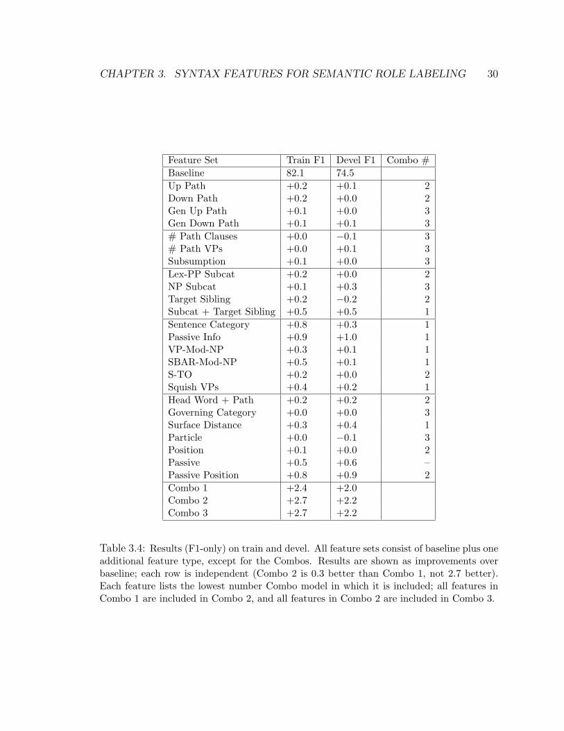
Table 3.4 shows results for adding each feature separately to the baseline system. For
almost all feature types, the results for training and development are consistent. The
path modification features are by far the most successful, particularly Passive Info
and Sentence Category. Of the eight features which improve over baseline on the
CHAPTER 3. SYNTAX FEATURES FOR SEMANTIC ROLE LABELING 30
Feature Set Train F1 Devel F1 Combo #Baseline 82.1 74.5Up Path +0.2 +0.1 2Down Path +0.2 +0.0 2Gen Up Path +0.1 +0.0 3Gen Down Path +0.1 +0.1 3# Path Clauses +0.0 −0.1 3# Path VPs +0.0 +0.1 3Subsumption +0.1 +0.0 3Lex-PP Subcat +0.2 +0.0 2NP Subcat +0.1 +0.3 3Target Sibling +0.2 −0.2 2Subcat + Target Sibling +0.5 +0.5 1Sentence Category +0.8 +0.3 1Passive Info +0.9 +1.0 1VP-Mod-NP +0.3 +0.1 1SBAR-Mod-NP +0.5 +0.1 1S-TO +0.2 +0.0 2Squish VPs +0.4 +0.2 1Head Word + Path +0.2 +0.2 2Governing Category +0.0 +0.0 3Surface Distance +0.3 +0.4 1Particle +0.0 −0.1 3Position +0.1 +0.0 2Passive +0.5 +0.6 –Passive Position +0.8 +0.9 2Combo 1 +2.4 +2.0Combo 2 +2.7 +2.2Combo 3 +2.7 +2.2
Table 3.4: Results (F1-only) on train and devel. All feature sets consist of baseline plus oneadditional feature type, except for the Combos. Results are shown as improvements overbaseline; each row is independent (Combo 2 is 0.3 better than Combo 1, not 2.7 better).Each feature lists the lowest number Combo model in which it is included; all features inCombo 1 are included in Combo 2, and all features in Combo 2 are included in Combo 3.

CHAPTER 3. SYNTAX FEATURES FOR SEMANTIC ROLE LABELING 31
Feature Set Train F1 Devel F1Combo 1 84.5 76.5- (Subcat + Target Sibling) 84.2 76.3- Sentence Category 84.2 76.3- Passive Info 83.9 75.9- VP-Mod-NP 84.3 76.3- SBAR-Mod-NP 84.5 76.4- Squish VPs 84.3 76.5- Surface Distance 84.4 76.3
Table 3.5: Results of removing features one at a time from Combo 1
training set by at least 0.3, five are in this group. Of these five, four are new; and two
of these (SBAR-Mod-NP and VP-Mod-NP) capture information that has not been
used by any previous system. The other three features which improve by at least this
much were Subcat + Target Sibling, Surface Distance, and Passive Position. The
sub-path and path statistic features do not perform well; none improve over baseline
by more than 0.2.
Based on these results, we consider three combination models. Combo 1 includes
the baseline features plus all features that improve over baseline on the training set by
at least 0.3: Subcat + Target Sibling, Sentence Category, Passive Info, VP-Mod-NP,
SBAR-Mod-NP, Squish VPs, and Surface Distance.3 Combo 2 includes all features
from Combo 1, plus Position and Passive Position, plus all features that improve over
baseline by at least 0.2: Up Path, Down Path, Lex-PP Subcat, Target Sibling, S-
TO, and HeadWord + Path. Combo 3 contains all features from Combo 2, plus all
remaining (non-redundant) features: Gen Up Path, Gen Down Path, # Path Clauses,
# Path VPs, Subsumption, NP Subcat, Governing Category, and Particle. Results
for these models are also shown in Table 3.4. Combo 1 improves substantially over the
baseline model and over the best single addition (Baseline + Passive Info). Combo 2
improves a bit over Combo 1 on both the training and development set, suggesting
that the added features do contribute something extra. Finally, Combo 3 does not
3We found that Passive Info and Passive Position are essentially redundant; we chose the betterof the two.

CHAPTER 3. SYNTAX FEATURES FOR SEMANTIC ROLE LABELING 32
System WSJ Brown CombBaseline 76.9 64.7 75.3Baseline + PassPos 77.7 65.3 76.1Combo 1 78.9 66.9 77.3Combo 2 79.2 66.2 77.5Punyakanok 79.4 67.8 77.9Toutanova Local 78.0 65.6 ∼76.3Toutanova Joint 79.7 67.8 ∼78.1Toutanova Joint Top 5 80.3 68.8 ∼78.8Surdeanu M2 77.2 67.7 76.0Surdeanu M3 76.5 65.4 75.0Surdeanu Combined 80.6 70.1 79.2
Table 3.6: F1 test scores. Combined F1 for Toutanova et al. (2008) not available; weestimate using a weighted average.
improve over Combo 2, which is not surprising considering that these features made
small or no difference even when added individually.
To check whether all seven of the additional features used in Combo 1 contributed to
the performance of the final system, we removed each of these features independently
from Combo 1. Results are shown in Table 3.5. For most of the features removing
the feature leads to a noticeable drop in performance. The main exception is SBAR-
Mod-NP: removing it barely affects performance, even though it gives a significant
increase when added to the basic feature set and does not obviously intersect with
any of the other features. It could be that Sentence Category, which (among other
things) indicates whether a relative clause has a subject, is providing some of the
same information that the SBAR-Mod-NP provides.
3.6 Comparison to State-of-the-art SRL Systems
Table 3.6 shows test results for four different feature sets: Baseline, Baseline + Passive
Position, Combo 1, and Combo 2. We include Baseline+PassPos because the Passive
Position feature is used by most high-performance SRL systems. The performance
of Baseline+PassPos is already quite good; in the CoNLL 2005 evaluation, it would

CHAPTER 3. SYNTAX FEATURES FOR SEMANTIC ROLE LABELING 33
System WSJ Brown CombCombo 2 79.2 66.2 77.5Combo 2 (reranked parses) 80.3 68.0 78.7Punyakanok 79.4 67.8 77.9Toutanova joint top 5 80.3 68.8 ∼78.8Surdeanu Combined 80.6 70.1 79.2
Table 3.7: Results using reranked parses
have placed at about the 75th percentile among evaluated systems. We also compare
to the three systems (Punyakanok et al., 2005; Toutanova et al., 2008; Surdeanu
et al., 2007) discussed in the previous section. For Toutanova et al. (2008), we report
results for three different models: Local, Joint, and Joint Top 5. Local is their local
classification model: it classifies each constituent independently and uses only the
top Charniak parse. Joint adds their reranking model, and Joint Top 5 combines
information from the five best Charniak parses. For Surdeanu et al. (2007), we show
results for M2, M3, and the final combined model.
To our knowledge, Combo 2 achieves the best reported results among systems that
(1) use only a single Charniak parse, and (2) classify each constituent independently.
The local model of Toutanova et al. (2008) is the best previous system subject to
these restrictions. This is presumably due to our detailed feature selection and our
new features. Among systems which use only a single Charniak parse, only the joint
model of Toutanova et al. (2008) outperforms Combo 2.
As a straightforward way of incorporating additional parse information, we also
ran our system using the 2006 version of the Charniak reranking parser (Charniak
& Johnson, 2005).4 This parser builds a list of the 50-best parses and reranks these
parses based on additional features of each parse. Thus, it is similar to the method
used by Toutanova et al. (2008) for using multiple parses (although the features are
obviously different). We simply used the top parse returned after reranking as input to
our system. Table 3.7 shows the results of Combo 2 applied to these parses, compared
to the best results for each of the three other systems. The use of the reranked parses
4Available at ftp://ftp.cs.brown.edu/pub/nlparser/reranking-parserAug06.tar.gz

CHAPTER 3. SYNTAX FEATURES FOR SEMANTIC ROLE LABELING 34
significantly improves our system, surpassing Punyakanok et al. (2005) and (almost)
matching Toutanova et al. (2008). Further improvements could likely be achieved by
using the self-trained parser described in McClosky et al. (2006).
Most likely, we could further improve our system by incorporating the ideas used
in these three systems (voting method of Punyakanok et al. (2005) for combining
multiple parses, joint modeling, and system combination). What the experimental
evaluation presented here shows is that our system (which includes both previously
suggested and new features) obtains the best performance when comparing purely
on local features. When using reranked parses, our system achieves performance
comparable to the best reported results on this task, while being comparatively easy
to implement (off-the-shelf parser and straight-forward learning/inference).

Chapter 4
Canonicalization for Semantic Role
Labeling
4.1 Introduction
A major problem with the standard approach to SRL is that the path feature can
be quite complicated. In the sentence “He expected to receive a prize for winning,” the
path from “win” to its ARG0, “he”, involves the verbs “expect” and “receive” and
the preposition “for”. The corresponding path through the parse tree likely occurs
a relatively small number of times (or not at all) in the training corpus. If the test
set contained exactly the same sentence but with “expected” replaced by “did not
expect”, we would extract a different parse path feature; therefore, as far as the
classifier is concerned, the syntax of the two sentences is totally unrelated. Many
verbs occur a small number of times in the training set, making the sparsity problem
even worse.
In Chapter 3, we experimented with several modifications to the path features
designed to help reduce sparsity. These included sub-path and path statistic features,
as well as the Squish VPs path modification feature. Of these, only the Squish VPs
feature gave a significant boost in performance, and this feature only handled one
specific source of sparsity related to inserting helper verbs.
35

CHAPTER 4. CANONICALIZATION FOR SEMANTIC ROLE LABELING 36
Verb Deep Subject Deep Objects wants Tom to eat an apple eat Tom an apple
Figure 4.1: Canonical forms for all verbs in “Tom wants to eat an apple.”
In this chapter, we propose a new approach based on canonical forms. The canonical
form for a sentence s and target verb v consists of two parts, either of which may
or may not be present: a deep subject, and a (possibly empty) ordered list of deep
objects. In cases where v has a syntactic subject, the deep subject is identical to the
syntactic subject. However, the deep subject is also defined in many cases when the
syntactic subject is missing. For example, in “Tom wants to eat an apple,” “eat” is
missing a syntactic subject but has deep subject “Tom.” Deep objects have a similar
relationship to syntactic objects. Figure 4.1 shows the canonical forms for all verbs
in “Tom wants to eat an apple.”
Suppose we are given a canonicalization system, a system that can extract the
canonical form for a given sentence s and target verb v. Our main idea is to perform
SRL on the canonical form, rather than on the original input sentence. The advantage
of this is that (by design) canonical forms remove (most of) the syntactic variability
of the original sentence.1 Thus, it is much easier to generalize between different
examples. For example, if we have only seen a particular verb in active form in the
training set, we may have difficulty when we see it in passive form in the test set.
However, the canonical form represents passive and active sentences in the same way,
so we will be more likely to be able to correctly label the passive sentence in the test
set.
In this chapter, we first define canonical form more precisely and discuss its rela-
tionship to previous work, mainly in linguistics. Second, we describe how we build a
1An example of variability which is not removed by our system is “He gave him the ball” vs. “Hegave the ball to him”.

CHAPTER 4. CANONICALIZATION FOR SEMANTIC ROLE LABELING 37
canonicalization system. Our system makes use both of hand-coded linguistic knowl-
edge and machine learning. It is also able to correctly model the recursive structure
of natural language. Third, we describe our canonical form SRL system. Fourth,
we describe how to train both the canonicalization and canonical-form SRL systems.
Since we do not have labeled data for the canonicalization system, we treat the correct
canonical form as a hidden variable, which allows us to train both systems using only
labeled SRL data. Finally, we evaluate our system on the CoNLL 2005 shared task,
showing that it performs competitively with standard SRL systems. As expected, our
system performs particularly well for verbs with a small amount of training data.
4.2 Canonical Forms
In the previous section, we informally defined a canonical form as containing a deep
subject and an ordered list of deep objects (either of which could be missing). We
have also implied that given a sentence s and a target verb v, there is a unique correct
canonical form. In this section, we will formalize the definition of correct canonical
form and give further examples of canonical forms.
Given s and v, the correct canonical form is the canonical form such that the deep
subject and all the deep objects are direct arguments of v. This is a simple notion
intuitively, but there are several issues which make it complicated in practice.
The basic idea of our approach is to define the correct canonical form based on the
semantic roles labeled in our data for the target verb v. Thus, the deep subject and
deep objects should all be labeled as arguments of v.
This still leaves open the question of which argument should be the deep subject. We
will not provide an exact criterion for determining the correct deep subject; instead,
we give an intuitive definition that covers nearly every case. The deep subject is the
argument of v which would be placed before the verb if we were to write a sentence
in which v was the main verb of the sentence. Typically, the deep subject appears
before v in the s, while the deep objects appear after v. Passive sentences are an
obvious but easily handled exception. As we will see, the lack of precise definition

CHAPTER 4. CANONICALIZATION FOR SEMANTIC ROLE LABELING 38
of the correct canonical form is not actually an issue for our system. However, if
we were to attempt to label gold-standard canonical forms, there would probably be
some rare cases that would need to be addressed.
There is one common situation where we wish to include a non-role constituent (at
least according to PropBank) in our canonical form. This is in the case of “it” as
in “It rained,” and the existential “there” in “There was rain.” In some sense these
words have no semantic content, so it is a somewhat arbitrary decision to label or
not label them. Our goal was to make the canonical form as “readable” as possible,
so we chose to include these two special cases in the canonical form.
4.2.1 Related Formalisms
One area of current research which has similarities with this work is Lexical-Functional
Grammars (LFGs) (Kaplan & Bresnan, 1982) (e.g., the XLE system2). LFGs and our
approach both attempt to abstract away from the surface level syntax of the sentence.
The relationship between the c-structure (syntactic structure, i.e., syntactic parse)
and the f-structure (grammatical function) in an LFG is similar to the relationship
between a sentence (or phrase) and the canonical form of that sentence, in that
both attempt to abstract away the particular syntactic instantiation present in the
sentence. The most obvious difference in our approach is that we use SRL data to
train our system, avoiding the need to have labeled data specific to our method.
Combinatory Categorial Grammars (CCGs) also build a representation abstracted
from the syntax of the sentence. In this method, a strong type system is introduced
which maps syntactic elements into typed functions. The semantic representation of
the sentence is built by recursively applying the functional representations of each
node in the parse. Similar to our method, a CCG parser analyzes a sentence re-
cursively, piece by piece. Following our work, Boxwell et al. (2009) implemented
an SRL system using features generated from a CCG parser. Our system signifi-
cantly outperforms their system on the CoNLL 2005 shared task (they report overall
2http://www2.parc.com/isl/groups/nltt/xle/

CHAPTER 4. CANONICALIZATION FOR SEMANTIC ROLE LABELING 39
F1 measure of 73.5% when using automatic parses). This could be partly because
we rely more heavily on the high-quality parses generated by the Charniak parser,
while their transformation-based features are extracted from a separated CCG parser.
Additionally, our “parsing” system, based on tree transformations, clearly differs in
many aspects from the approach taken by CCG.
Lexicalized Tree-Adjoining Grammars (LTAGs) also implicitly maintain a kind of
underlying representation. LTAGs have two types of syntactic operations: substitu-
tion (which is essentially the same as the substitution rule in a context-free grammar)
and adjunction. Adjunction allows a tree to be inserted in the middle of another tree.
For example, the sentence “I go,” by using the adjunction rule with the phrase “want
to,” can generate the sentence “I want to go.” The LTAG parse of this sentence will
include the “simplified” sentence “I go,” which can be used as an abstracted repre-
sentation of the arguments of “go.” Recently, Liu et al. (2010) built a system based
on an LTAG parser which has several similarities with our work. Their system treats
the correct LTAG derivation as a hidden variable and then learns a model based on
maximizing performance on SRL data. As in our system, they take the top Charniak
parse as given and learn a model based on this parse. They report very impressive
results on the CoNLL 2005 task, achieving an overall F1 of 89.59, 9 F1 points higher
than the next best system.
In terms of the specific algorithms in our system, some work has been done on
packed representations. Maxwell III & Kaplan (1995) propose a packed representation
similar to the data structure presented in Section 4.7, while Geman & Johnson (2002)
present an inference algorithm which operates on this type of data structure. However,
to our knowledge, the algorithm we present for constructing our packed representation
(described in Section 4.7) has not been explored in previous work.
Another group of related work outside of SRL focuses on summarizing sentences
through a series of deletions (Jing, 2000; Dorr et al., 2003; Galley & McKeown,
2007). In particular, the latter two works iteratively simplify the sentence by deleting
a phrase at a time. Our approach differs from these works in several important ways.
First, our transformation language is not context-free; it can reorder constituents and

CHAPTER 4. CANONICALIZATION FOR SEMANTIC ROLE LABELING 40
then apply transformation rules to the reordered sentence. Second, we are focusing on
a somewhat different task; these works are interested in obtaining a single summary
of each sentence which maintains all “essential” information, while we produce a
canonical form that may lose semantic content but aims to contain all arguments of a
verb. Finally, training our model on SRL data allows us to avoid the relative scarcity
of parallel simplification corpora and the issue of determining what is “essential” in
a sentence.
Another related area of work within the SRL literature is that on tree kernels
(Moschitti, 2004; Zhang et al., 2007). Like our method, tree kernels decompose the
parse path into smaller pieces for classification. Our model can generalize better
across verbs because it first generates canonical forms, then classifies the resulting
canonical forms. Also, through iterative simplifications we can discover structure
that is not immediately apparent in the original parse.
Johnson (2002) and Levy & Manning (2004) present algorithms for finding non-
local dependencies given a parse tree. These methods are similar to our system in
that a significant portion of the work our system does is resolving these kinds of
long-range dependencies in order to generate canonical forms. The most significant
difference in our work is that we incorporate this idea into a semantic role labeling
system, where we are able to gain from increased generalization due to resolving
these dependencies. Additionally, in order to normalize syntax as much as possible,
our system handles syntactic structures not covered by these systems. For example,
rewriting passive sentences as active sentences is not an example of resolving non-
local dependencies, but it is an important step in generating a canonical form. An
interesting area for future work is incorporating the detailed analyses in these works
into a transformation-based SRL system.
4.3 Canonicalization System
In this section we describe the system we built to automatically extract canonical
forms from sentences.

CHAPTER 4. CANONICALIZATION FOR SEMANTIC ROLE LABELING 41
4.3.1 System Overview
The basic building blocks of our system are transformation rules. Roughly speak-
ing, each transformation rule handles one specific kind of syntactic construct. The
transformation rule can only be applied to sentences containing that construct. When
applied, the rule rewrites the sentence so that it no longer uses that construct. For ex-
ample, one of our rules converts a passive sentence into an active sentence. This rule,
when applied to the passive sentence “I was given a chance,” outputs the transformed
sentence “Someone gave me a chance.” (Someone is a placeholder that indicates that
the subject of the active sentence is missing).
For our system to work well, we need a set of rules which covers as many common
syntactic patterns as possible. One approach would be to try to automatically extract
these rules from text. However, as already mentioned, we do not have data labeled
with canonical forms, much less data labeled with a step-by-step series of transfor-
mations. We could try to automatically infer rules from labeled SRL data, but this
approach is very difficult, requiring a search over a vast space of possible rules.
Instead, we chose to hand-construct a rule set that encodes a large amount of
human-level linguistic knowledge. The rule set was built through iterative develop-
ment on (training) data. Rules were added one-by-one or in groups until the rule set
was capable of generating, for most (> 95%) of the sentences in the training set, a
canonical form containing all labeled arguments of each target verb.3
While hand-coding rules is an effective way to inject knowledge into the system, we
also need a strategy for choosing which rules to use. A simple deterministic approach
is unlikely to work well, because for many sentences, there are many possible rules
which can be applied. For example, in the sentence “I wanted the chicken to eat,”
one rule puts “I” as the subject of “eat,” while another puts “chicken” as the subject
as “eat.” For this reason, we took a machine learning approach to deciding how to
apply the rules, which determines which rule to use based on features of the sentence
3Note that such a canonical form is not necessarily the correct canonical form, because it mightcontain non-argument constituents. However, we considered these canonical forms “good enough”as far as the SRL system was concerned.

CHAPTER 4. CANONICALIZATION FOR SEMANTIC ROLE LABELING 42
* - 1
NP - 2 VP - 3
S
NP VP
VBD
slept
I slept
I
S
NP VP
VBD
ate
NP
a sandwich
I
I ate a sandwich
Figure 4.2: Example tree pattern and matching constituents
S
NP
I slept
I
S
NP
VP
VBD
ate
NP
a sandwich
I
I ate a sandwich
VP
VBD
slept
Figure 4.3: Result of applying add-child-end(3,2) in Figure 4.2. Note that the tree patternin Figure 4.2 specifies that in each sentence, the label 3 refers to the matched VP, whilethe label 2 refers to the matched NP. Thus, add-child-end(3,2) moves the matched VP tobe the final child of the matched NP.
and target verb.
4.3.2 Transformation Rules
A transformation rule consists of two parts: a tree pattern and a series of transforma-
tion operations. It takes as input a parse tree, and outputs a new, transformed parse
tree. The tree pattern determines whether the rule can be applied to a particular
parse and also identifies what part of the parse should be transformed. The trans-
formation operations actually modify the parse. Each operation specifies a simple
modification of the parse tree.
A tree pattern is a tree fragment with constraints on each node. For example,

CHAPTER 4. CANONICALIZATION FOR SEMANTIC ROLE LABELING 43
Figure 4.2 is a tree pattern that matches any constituent in the parse tree which has
an NP and a VP as children. Alongside is pictured two constituents which match
this pattern. The tree pattern also assigns numerical labels to each of the matched
nodes, which are used by the transformation operations as described below.
Formally, a tree pattern node X matches a parse-tree node A if: (1) All constraints
of node X (e.g., constituent category, head word, etc.) are satisfied by node A. (2)
For each child node Y of X, there is a child B of A that matches Y; two children of
X cannot be matched to the same child B. (3) All constraints between children are
satisfied — for example, the pattern could require that child B comes before child
C in the parse. There are no other requirements. A can have other children besides
those matched, and leaves of the rule pattern can match to internal nodes of the
parse (corresponding to entire phrases in the original sentence). For example, the
same rule can be used to transform both “Tom wanted to eat” and “Tom wanted to
eat a sandwich” (into “Tom ate” and “Tom ate a sandwich”). The insertion of the
phrase “a sandwich” does not prevent the rule from being applied.
A transformation operation is a simple step that is applied to the nodes matched by
the tree pattern. For example, the “add-child-end” transformation operation applied
to the pair of nodes (X,Y) removes X from its current parent and adds it as the final
child of Y. Figure 4.3 shows an example of applying this operation to the parses in
Figure 4.2.
Figure 4.4 shows a complete transformation rule that depassivizes a sentence, as
well as the result of applying it to the sentence “I was given a chance.” The transfor-
mation steps are applied sequentially from top to bottom. Any nodes not matched
are unaffected by the transformation; they remain where they are relative to their
parents. For example, “chance” is not matched by the rule and thus remains as a
child of the VP headed by “give.”
Note that a single transformation operation may not correspond to a linguistically
sensible transformation of the parse tree. However, the transformation rules were
designed so that the entire sequence of transformation operations for a particular
rule should correspond to a sensible transformation of the input parse. Thus, the

CHAPTER 4. CANONICALIZATION FOR SEMANTIC ROLE LABELING 44
NP-7
[Someone] VB-5 NP
VP-4
give chance
NP-2
I
VB-5 NP
VP-4
give chance
NP-2
I
S-1S-1
NP-2 VP-3
VB*-6
VBN-5be
VP-4
TransformedRule
Replace 3 with 4Create new node 7 – [Someone]Substitute 7 for 2Add 2 after 5Set category of 5 to VB
S
NP VP
VBD
VBN NPwas
VP
given chance
I
Original
Figure 4.4: Rule for depassivizing a sentence
intermediate steps during the application of the transformation operations may not
be syntactically well-formed, but the final output parse should be (assuming the
transformation rule is well-designed).
4.3.3 Rule Set
Altogether, we currently have 154 (mostly unlexicalized) rules. Our general approach
was to write very conservative rules, i.e., avoid making rules with low precision. We
did this mainly because low-precision rules can quickly lead to a large blow-up in the
number of ways to generate a canonical form from a given input sentence/target verb
pair. Table 4.1 shows a summary of our rule-set, grouped by type. Note that each row
lists only one possible sentence and simplification rule from that category; many of
the categories handle a variety of syntax patterns. The two examples without target
verbs are helper transformations; in more complex sentences, they can enable further
simplifications. Another thing to note is that we use the terms Raising/Control (RC)
very loosely to mean situations where the subject of the target verb is displaced,
appearing as the subject of another verb.
There are two significant pieces of “machinery” in our current rule set. The first is
the idea of a floating node, used for locating an argument within a subordinate clause.

CHAPTER 4. CANONICALIZATION FOR SEMANTIC ROLE LABELING 45
SimplifiedOriginal#Rule Category
I atethe food.Float(The food) I ate.
5Floating nodes
He slept.I said he slept.4Sentence extraction
Food is tasty.Salt makes food tasty.
8“Make” rewrites
The total includestax.
Includingtax, the total…
7Verb acting as PP/NP
John has a chance to eat.
John’s chance to eat…
7Possessive
I will eat.Will I eat?7Questions
I will eat.Nor will I eat.7Inverted sentences
Float(The food) I ate.
The food I ate…8Modified nouns
I eat.I have a chance to eat.
7Verb RC (Noun)
I eat.I am likely to eat.6Verb RC (ADJP/ADVP)
I eat.I wantto eat.17Verb Raising/Control (basic)
I eat.I must eat.14Verb Collapsing/Rewriting
I ate.I ateand slept.8Conjunctions
John is a lawyer.John, a lawyer, …20Misc Collapsing/Rewriting
A car hitme.I was hitby a car.5Passive
I sleptThursday.Thursday, I slept.24Sentence normalization
Table 4.1: Rule categories with sample simplifications. Target verbs are underlined.

CHAPTER 4. CANONICALIZATION FOR SEMANTIC ROLE LABELING 46
For example, in the phrases “The cat that ate the mouse”, “The seed that the mouse
ate”, and “The person we gave the gift to”, the modified nouns (“cat”, “seed”, and
“person”, respectively) all should be placed in different positions in the subordinate
clauses (subject, direct object, and object of “to”) to produce the phrases “The cat
ate the mouse”, “The mouse ate the seed”, and “We gave the gift to the person”.
We handle these phrases by placing a floating node in the subordinate clause which
points to the argument; other rules try to place the floating node into each possible
position in the sentence.
The second construct is a system for keeping track of whether a sentence has a
subject, and if so, what it is. A subset of our rule set normalizes the input sentence
by moving modifiers after the verb, leaving either a single phrase (the subject) or
nothing before the verb. For example, “Before leaving, I ate a sandwich” is rewritten
as “I ate a sandwich before leaving”. In many cases, keeping track of the presence or
absence of a subject greatly reduces the set of applicable transformation rules.
For example, when placing floating nodes as described above, if a subject has been
identified in the subordinate clause (e.g., in “the mouse the cat ate”, the subordinate
clause “the cat ate” has a subject, “the cat”), the floating node cannot be placed in
the subject position. Note that in some cases, the presence and identity of a subject
is ambiguous; our canonicalization system will generate each candidate normalization
of the sentence and will (hopefully) learn to choose the correct normalization.
As mentioned above, our rule set was developed by analyzing performance and
coverage on the PropBank WSJ training set. Neither the development set nor (of
course) the test set were used during rule creation.
4.3.4 Sequences of Rules
A single transformation rule handles a single syntactic construct. In many sentences,
there are many different syntactic structures, often nested in a recursive fashion. To
handle this, we can simply apply a sequence of rule transformations, one at a time.
Assuming our rule set is written well, the output of each transformation rule should

CHAPTER 4. CANONICALIZATION FOR SEMANTIC ROLE LABELING 47
I did not like the decision that was made.
The decision was made.
Someone made the decision.
Rule: Floating Nodes
Rule: Depassivize
Float(The decision) was made. Rule: Modified Nouns
Figure 4.5: Iterative transformation rule application
be a syntactically valid parse, and so other transformation rules should in turn be
applicable to the resulting parse. Figure 4.5 shows a series of rules applied to the
sentence “I did not like the decision that was made,” with target verb “made.”
We followed an important design principle related to sequences of rules when de-
signing our rule set: we tried to maximize reuse of each transformation rule as much
as possible. For example, one of our rules transforms “Bob has a chance to eat,” into
“Bob eats.” Consider the sentence “Bob’s chance to eat has passed.” One option
would be to write a separate, similar rule that applies to the “X’s Y to Z” construc-
tion instead of the “X has a Y to Z” construction. Instead, we wrote a new rule which
rewrites any possessive sentence using the verb “have.” This rule transforms “Bob’s
chance to eat has passed,” into “Bob has a chance to eat.” We can now apply the
earlier rule to this new transformed sentence. By breaking complex transformations
down into smaller building blocks, we increase the number of training examples for
each transformation rule, allowing us to better learn when to use them.
Another issue worth mentioning at this point is that many of the steps do lose
some semantic information. Clearly, having a chance to eat is not the same as eating.
However, since our goal is to label the arguments of the verb (which in this case is
simply the Eater, “I”), it is not important to maintain this information. Furthermore,

CHAPTER 4. CANONICALIZATION FOR SEMANTIC ROLE LABELING 48
it is possible to modify the rule set to maintain this kind of information. For example,
we could attach annotations to each node in the parse which keep track of information
removed by previous transformation steps.
We consider a series of rules to be “finished” when it produces a parse satisfying
the following constraints:
i. The root node X has category S
ii. X has a child Y with category VP
iii. X has exactly one child Z (the subject) occurring before Y. Z may be empty as
described above.
iv. The main verb of the VP constituent rooted at Y is the target verb v.
We can construct a canonical from this parse in the obvious way: Z becomes the
deep subject of the canonical form, and all children of Y besides v become the deep
objects.
4.4 Producing Canonical Forms
For many sentence/target verb pairs (s,v), there are many possible canonical forms
that can be generated using our rule set. We now describe how to efficiently generate
the set of all possible candidate canonical forms for (s,v). At a high level, the algo-
rithm is very simple. We maintain a set of derived parses S which is initialized to
contain only the original, untransformed parse. One iteration of the algorithm con-
sists of applying every possible matching transformation rule to every parse in S, and
adding all resulting parses to S. With carefully designed rules, repeated iterations
are guaranteed to converge; that is, we eventually arrive at a set S such that if we
apply an iteration of rule application to S, no new parses will be added. Note that
this process does not refer to the target verb v, which means that we only need to
do it once per sentence. To find canonical forms for v, we simply look through S for
parses satisfying the conditions from the previous section.

CHAPTER 4. CANONICALIZATION FOR SEMANTIC ROLE LABELING 49
!"
!#"
!##"
!###"
!####"
!#####"
#$!"
%$&"
'$!&"
!'$(#"
(!$!#&"
!#'$%)!"
%)%$'*!"
'*%$!)'%"
!)'+$((,)"
((,,$!!(%'"
Figure 4.6: Number of (s,v) pairs (Y-axis)vs. number of canonical form/rule set pairs(buckets on X-axis)
!"!#"
!##"!###"
!####"!#####"
#$%"
&$'"
!#$&%"
&&$!#("
!#)$&*!"
&*%$!!##"
!!#!$&(&'"
&(*#$!!&+("
!!&+)$&)(('"
&)()#$!!+*'!"
Figure 4.7: Number of (s,v) pairs (Y-axis) vs. number of canonical form/ruleset/labeling triples (buckets on X-axis)
This generation procedure is conceptually simple but computationally quite expen-
sive. Implemented naively, we would need to copy the entire parse tree at each step,
and in general, this procedure could generate an exponential number of transformed
parses. The first issue can be solved, and the second alleviated, using a dynamic-
programming data structure similar to the one used to store parse forests (as in a
chart parser). This data structure is not essential for exposition; we delay discussion
until Section 4.7. Even given this compact storage, the data structure can become
exponential; in practice, however, the size of the compact representation is sometimes
large but manageable (statistics presented below).
Our system keeps track of the set of rules used to generate a canonical form, but
not the order in which the rules were applied. If two rules affect a different part of
the parse, they can be reordered arbitrarily; for this reason, in most cases, keeping
track of rule application order is neither important nor feasible. Similarly, it often
happens that one rule transforms a part of the parse which is discarded by a later
transformation. For this reason, we maintain only minimal subsets of rules which
generate a particular canonical form.
Subject to the rule set collapsing described in the previous paragraph, on the Prop-
Bank training set, the largest number of canonical form/rule set pairs generated for

CHAPTER 4. CANONICALIZATION FOR SEMANTIC ROLE LABELING 50
a particular sentence/target verb pair was just under 5000. Figure 4.6 shows a his-
togram of number of canonical form/rule pairs across all sentence/target verb pairs.
Note that both axes are on a log scale.
4.5 Labeling Canonical Forms
For a particular sentence/target verb pair (s, v), the output from the previous section
is a set Csv = {csvi }i of possible canonical forms. Although labeling a canonical form
is easier than labeling the original sentence, there are still many choices to be made.
Additionally, the labeling task is complicated by the fact that for some sentences,
there are no correct canonical forms. This happens primarily because of errors in the
automatic parser, which can cause arguments to be missing from the canonical form
and non-arguments to erroneously appear in the canonical form.
On the training set, we now extract a set of role patterns Gv = {gvj }j for each
verb v. For example, the role pattern for “give” in “I gave him a sandwich” is
ggive1 = {ARG0 = Subject NP, ARG1 = Object NP2, ARG2 = Object NP1}. Note
that this is one atomic pattern; thus, we are keeping track not just of occurrences of
particular roles in particular places in the simple sentence, but also how those roles
co-occur with other roles.
For a particular simple sentence csvi , we apply all extracted role patterns gv
j to csvi ,
obtaining a set of possible role labelings. We call a canonical form/role labeling pair a
labeled canonical form and denote the set of candidate labeled canonical forms Lsv =
{lsvk }k. Note that a given pair csvi , gv
j may generate more than one labeled canonical
form, if there is more than one way to assign the elements of gvj to constituents in
csvi . Also, for a sentence s there may be several labeled canonical forms that have the
same assignment of roles to constituents. In particular, there may be several labeled
canonical forms that assign the correct labels to all constituents; we denote this set
Ksv ⊆ Lsv.
As mentioned earlier, we do not have access to the correct canonical forms (or the
sequence of rules which generates it). Instead, we use the set Ksv as our notion of

CHAPTER 4. CANONICALIZATION FOR SEMANTIC ROLE LABELING 51
correctness. This will allow us to train our model using only labeled semantic role
data. Note that Ksv does not exclude canonical forms that include constituents that
were not labeled as arguments.
On the PropBank training set, the number of canonical form/rule set/labeling
triples generated for a particular sentence/target verb pair ranged from 1 to 120,000.
The median number of triples was 13, so the majority of sentences are not expen-
sive computationally. Figure 4.7 shows a histogram of number canonical form/rule
set/labeling triples across all sentence/target verb pairs.
4.6 Probabilistic Model
We now define our probabilistic model. Given a (possibly large) set of candidate
labeled canonical forms Lsv, we need to select a (hopefully correct) one. We assign
a score to each candidate based on its features: which rules were used to obtain the
canonical form, which role pattern was used, and which constituents were assigned
to which roles. A log-linear model then assigns probability to each labeled canonical
form equal to the normalized exponential of the score.
The first type of feature is which rules were used to obtain the canonical form.
These features are indicator functions for each possible rule. Thus, we do not cur-
rently learn anything about interactions between different rules. A possible extension
of this feature type includes lexicalized versions of each rule. For example, for deter-
mining control, the main verb in the sentence is important. Unfortunately, due to
computational limitations, we were not able to explore this extension.
The second type of feature is an indicator function of the role pattern used to
generate the labeling. This allows us to learn that “give” has a preference for the
labeling {ARG0 = Subject NP, ARG1 = Postverb NP2, ARG2 = Postverb NP1}.
Our final features are analogous to those used in semantic role labeling, but greatly
simplified due to our use of canonical forms: head word of the constituent; category
(i.e., constituent label); and position in the canonical form. Each of these features
is combined with the role assignment, so that each feature indicates a preference

CHAPTER 4. CANONICALIZATION FOR SEMANTIC ROLE LABELING 52
!"#$%&%'!()*%+$,-%."/-%&%0"12%!"#$%&%'!()*%345%&%63%!"#$%&%'!()*%3"789"2%&%5:;<%63%
!:#$%&%=$>,778?8@$%
3,A$/2%&%B'!()%&%5:;<%63*%'!(C%&%4;<%63D*%'!(D%&%4;<%63CE%
!"#$%&%'!(C*%+$,-%."/-%&%7,2-.8F1%!"#$%&%'!(C*%345%&%63%!"#$%&%'!(C*%3"789"2%&%4;<%63D%
!"#$%&%'!(C*%+$,-%."/-%&%G%!"#$%&%'!(C*%345%&%63%!"#$%&%'!(C*%3"789"2%&%4;<%63C%
Figure 4.8: Features for canonical form (Subject = “John”, Objects = {“me”,“a sand-wich”}) and labeling (ARG0 = “John”, ARG1 = “a sandwich”, ARG2 = “I”).
for a particular role assignment (i.e., for “give”, head word “sandwich” tends to be
ARG1). For each feature, we have a verb-specific and a verb-independent version,
allowing sharing across verbs while still permitting different verbs to learn different
preferences. The set of extracted features for the sentence “I was given a sandwich
by John” with canonical form (Subject = “John”, Objects = {“me”,”a sandwich”})and labeling (ARG0 = “John”,ARG1 = “a sandwich”,ARG2 = “I”) is shown in
Figure 4.8. We omit verb-specific features to save space. Note that we “stem” all
pronouns (including possessive pronouns).
For each candidate labeled canonical form lsvk , we extract a vector of features f svk as
described above. The probability of lsvk with respect to a weight vector w is defined
to be P (lsvk ) = ewTfsvkP
k′ ewTfsv
k′.
Our goal is to maximize the total probability assigned to any lsvk ∈ Ksv. Therefore,
for each sentence/verb pair (s, v), we want to increase∑
lsvk ∈Ksv P (lsvk ). This expres-
sion treats the canonical form and the sequence of rules used to extract it as a hidden
variable that is summed out. Taking the log, summing across all sentence/verb pairs,

CHAPTER 4. CANONICALIZATION FOR SEMANTIC ROLE LABELING 53
and adding L2 regularization on the weights to prevent overfitting, we have our final
objective F (w): ∑s,v
log
∑lsvk ∈Ksv ewTfsvk∑lsvk′ ∈Lsv ewTfsv
k′
− wTw
2σ2
We train our model by optimizing the objective using standard methods, specifically
L-BFGS (Liu & Nocedal, 1989). Due to the summation over the hidden variable
representing the choice of canonical form, our objective is not convex. Thus, we are
not guaranteed to find a global optimum. This means that initialization may affect
the final results; in practice we obtained good results using the default initialization of
setting all weights to 0. This may be because many sentences have only one canonical
form that admits a correct role labeling and only one sequence of rules that generates
this canonical form. Thus, we effectively have a large supervised set that helps to
constrain the learned parameters and to guide the model in a good direction.
Consider the derivative of the likelihood component with respect to a single weight
wl:
∑lsvk ∈Ksv
f svk (l)
P (lsvk )∑lsvk′ ∈Ksv
P (lsvk′ )−∑
lsvk ∈Lsv
f svk (l)P (lsvk )
where f svk (l) denotes the lth component of f sv
k . This formula is positive when the
expected value of the lth feature is higher on the set of correct simple labelings Ksv
than on the set of all simple labelings Lsv. Thus, the optimization procedure will tend
to be self-reinforcing, increasing the score of correct simple labelings that already have
a high score.
4.7 Simplification Data Structure
Recall that in order to generate all possible canonical forms for an input sentence s,
we iteratively build a set S of transformed parses. At each step, we try applying every
rule in our rule set to every parse in S. Implemented naively, this requires copying

CHAPTER 4. CANONICALIZATION FOR SEMANTIC ROLE LABELING 54
S
NP
I will go.
I
VP
VB
go
I go.
VB
VB
go
VP
VP
will
S
NP
I
Figure 4.9: Separate parses for “I will go” and “I go”
the entire parse at each step. Furthermore, the number of possible transformed parses
can be exponentially large. In this section we describe a data structure that addresses
both of these computational issues.
4.7.1 Sharing Structure
Suppose we begin with “I will go” and then apply a transformation rule that removes
the helper verb “will”, yielding “I go”. S now contains two parses, one for “I will go”
and one for “I go”. The simplest way to represent S is to store both parses separately,
as in Figure 4.9.
However, it is clear that the two parses share a lot of structure. The root node
(labeled S) and its first child subtree are the same in both parses. We can represent
this shared structure through the use of a choice node. Figure 4.10 shows our two
example sentence stored using a choice node, represented as “OR” inside a circle. We
refer to a parse containing choice nodes as a parse forest. The set of parses represented
by a particular parse forest corresponds to all possible ways of picking a choice for
each choice node. Thus, in Figure 4.10, we are storing two parses, one where we
choose the child constituent “will go” and one where we choose “go.”
There is even more shared structure: both parses contain the constituent VP–VB–
go. We can take advantage of this shared structure simply by pointing the second

CHAPTER 4. CANONICALIZATION FOR SEMANTIC ROLE LABELING 55
S
NP
VB
VB
go
VP
I will go. AND I go.
I
VP
will
VP
VB
go
OR
Figure 4.10: Using a choice node toshare structure
S
NP
VB
VB
go
VP I
VP
will
OR
I will go. AND I go.
Figure 4.11: Sharing structure using adirected acyclic graph
child of the choice node at the appropriate place in the first child. The resulting data
structure is shown in Figure 4.11. Note that our data structure is no longer a tree
(instead, it is a directed acyclic graph), but we will continue to refer to it as a parse
forest. The process for recovering the set of parses is exactly the same as before.
We say that a parse forest is valid if it has the property that given a set of choices
for each choice node, the resulting structure is a tree. Put another way, every cycle
in the parse forest must go through at least two children of some choice node (and
thus the cycle can never be present given choices for all choice nodes).
The parse forest data structure is basically the same data structure as the chart
used in chart parsing algorithms such as the CKY algorithm (Kasami, 1965; Younger,
1967). The primary difference is that a chart parse stores parses that differ only on
internal labels and structure, while we store parses that represent different sentences.
This makes the problem of finding a good (i.e., small) parse forest for a given set of
parses much more difficult.
Recall that there were two issues we wished to address. The first was to avoid
copying the entire parse every time we applied a rule. It is not hard to see that
when applying a rule, we only need to create new nodes in the parse tree for every
node in the transformed parse that is actually modified by the transformation rule.
Typically, a transformation rule modifies only a subtree of the entire parse. We can

CHAPTER 4. CANONICALIZATION FOR SEMANTIC ROLE LABELING 56
then simply replace the original root of this subtree with a new choice node, which
points to both the untransformed version of the subtree and the newly transformed
version (as in Figure 4.10). Thus, we do not need to copy anything outside of the
subtree. Similarly, any descendants of nodes modified by the transformation rule do
not need to be copied, because we can have both the original and transformed versions
of the subtree point to the same descendants (as in Figure 4.11).
The second issue was to avoid producing an exponential number of transformed
sentences. Consider the sentence “I will eat and I will drink and I will play and . . . ”
Each subsentence can be transformed to remove the modal verb “will.” This yields an
exponential number of transformed sentences in the length of the parse. However, we
can easily represent all such transformed sentences compactly by representing each
subsentence as in Figure 4.11.
4.7.2 Rule Application
In order to maintain the advantages of the parse forest data structure, we need to be
able to apply transformations without expanding the set of sentences represented by
the parse forest. Fortunately, there is a straightforward way to do this.
Given a single parse tree, we apply a rule by first matching the tree pattern against
a subtree of the parse and then applying the transformation operations. For concrete-
ness, assume that we match the tree pattern top down — first we find a node that
matches the constraints on the root of the tree pattern, then we match the children of
the root, then their children, etc. We can do essentially the same in the parse forest.
The only difference is what happens when a choice node is reached. In this case, we
simply try matching against each possible child. This process could potentially be
exponential in the size of the tree pattern if there were a choice node at each level.
In practice, this is not an issue because our tree patterns all have under ten nodes,
and most nodes in the parse forest are not choice nodes.
After this matching process, we end up with a set of expanded subtrees (note that
we stop expanding the parse forest once we get to leaves of the tree pattern, since we

CHAPTER 4. CANONICALIZATION FOR SEMANTIC ROLE LABELING 57
can share the part of the parse forest below this point). We apply the transformation
operations to each of these subtrees, yielding a set of new subtrees. We then add
a new choice node at the root of the transformed subtree pointing to all of these
subtrees.
The result of this procedure is to apply the given transformation to all parses that
share this particular part of the parse forest. Thus, by repeating this process for all
rules and all nodes in the parse forest, we guarantee that we try all possible rules
on all possible parses. Any given step of this procedure only increases the number
of nodes in the parse forest by (number of nodes in the tree pattern) * (number of
expanded matched subtrees).
While this procedure is reasonably efficient, it can still be improved. For example,
suppose we have a parse forest representing the sentences “Bob was hit by a car” and
“Bob was hit by a truck”, stored as “Bob was hit by a car OR a truck”. If we apply
the depassivization rule to this sentence, we first expand out the entire parse (since
the root of the tree pattern for the depassivize rule matches the S node at the root
of the parse forest). We then apply the depassivization rule to each separately and
replace the root of the parse forest with an OR node pointing to each transformed
sentence as well as the original parse forest. We clearly can do much better than
this: the (transformed) sentences “A car hit Bob” and “A truck hit Bob” can be
represented as “A car OR a truck hit Bob”. Furthermore, both “a car OR a truck”
and “Bob” can be shared between the passive and active versions.
There are two useful heuristics we can apply to compactify the parse forest. The first
is to merge nodes from the bottom up. Starting at the leaves of the nodes matched
by the tree pattern. we check to see if the nodes were changed by the transformation
operations. If not, we can remove all but one of the copies of this node. We can
repeat this process, merging nodes until we get to a point where the nodes differ.
The second heuristic merges nodes top down. To guarantee we do not change the
parse forest, we need two conditions to hold. First, the two merged nodes must have
the same parent — otherwise, when we merge them, we will effectively create extra
edges in the parse forest. Second, the merged nodes must differ on at most one child.

CHAPTER 4. CANONICALIZATION FOR SEMANTIC ROLE LABELING 58
If these conditions hold, then we can merge the nodes, replacing the differing child
with a choice node that points to each variant of that child.
Suppose we want to compress the sentences “Alice ate” and “Alice ran”. Since
these sentences differ in only one place (the verb), we can compress them as “Alice
ate OR ran”. However, consider the sentences “Alice ate” and “Bob ran”. If we were
to compress as “Alice OR Bob ate OR ran”, we would have erroneously added the
sentences “Alice ran” and “Bob ate” to our set.
These two heuristics are enough to fix the problems discussed above when depas-
sivizing a sentence; in practice, they greatly reduce the final size of the parse forest.
The advantage of all the compression methods mentioned so far is that they only look
at the part of the parse forest currently being transformed. We also implemented a
very simple global reduction step that looks for nodes that are identical (identical
labels, words, and children). While further compression of the parse forest is often
possible through further examination of the entire parse forest, we found that these
steps (the two local heuristics plus the simple global step) were enough to keep the
parse forest reasonably small.
The top-down merge actually handles another issue not yet mentioned. To produce
the set of all canonical forms for a given input parse, we repeatedly apply rules to
nodes in the parse forest as described above. In doing this, we may produce a given
parse multiple times. In most cases, the top-down merge will automatically remove
the copies by merging them back into the forest.
There are various ways in which our compression heuristics could be improved.
One example would be to match entire “forests” of subtrees at once. For example,
if a passive sentence has two different possible NPs for its (syntactic) subject, the
current algorithm transforms each separately (hopefully recombining them in the
top-down compression step). Instead, since the depassivizing rule only requires an
NP, we could transform both at the same time, never needing to recombine them.
Our current algorithm has difficulty when there are multiple independent choices for
a particular rule; this optimization would fix this problem.

CHAPTER 4. CANONICALIZATION FOR SEMANTIC ROLE LABELING 59
4.7.3 Adding Rule Information
There is one additional detail of our parse forest generation procedure. Recall that
our probabilistic model is based on the set of rules used to generate a given canonical
form. Thus, we need to keep track of the rules used to generate each parse, but we
want to avoid explicitly representing every parse. It turns out that we can simply
attach rule identifiers to the edges of the parse forest. The set of rules which was
used to generate a given parse is simply the set of rules on the edges of that parse.
The method for doing this does somewhat complicates the construction of the parse
forest.
Recall that when we apply a transformation to a subtree of the parse forest, we
add all transformed versions of the subtree as children of a new choice node which
replaces the root of the subtree. To incorporate rule information into the parse forest,
we add a label to each of the edges from the transformed subtrees to the choice node
with the just-applied rule.
Furthermore, when we expand the subtree while matching the tree pattern, we also
need to keep track of all rules that are labels of edges in the matched subtree. We
then add all of these rules to the root of the matched subtree, adding them to the
same edge where we add the newly-applied rule. This ensures that we remember that
these rules were used to produce this subtree.
When applying our compression heuristics, we now must take into account the
edge labels. The bottom-up merge stays the same, except that the edge labels of all
children must also be the same. However, the top-down merge now becomes more
complicated, because in some cases we want to push edge labels back down the graph
in order to better compress the tree.
One way to explain the complication of the merge step is that when we apply a
rule to produce a new subtree, it is arbitrary exactly which edges we label in the
new subtree. This is because the only constraint is that each tree represented by the
parse forest is labeled with the correct set of rules; it does not matter which edges
are labeled. Thus, we have some flexibility in where we place the edges, so we have

CHAPTER 4. CANONICALIZATION FOR SEMANTIC ROLE LABELING 60
to solve a small optimization problem in order to decide which assignment of rules to
edges allows us to most compress the parse forest. Fortunately, this optimization is
relatively straightforward to solve.
4.7.4 Inference and Learning
Again, in order for the parse forest to be useful, we must be able to do inference
(probability queries about canonical forms) and learning (optimizing the parameters
of our model) without expanding the set of parses represented by the parse forest.
In this case, we can use a relatively straightforward extension of the inside-outside
algorithm for chart parses; a similar algorithm was proposed by Geman & Johnson
(2002). This allows us to compute statistics of the nodes of the parse forest in time
linear in the number of edges in the parse forest. This is sufficient to make both
inference and learning efficient in our model.
4.8 Experiments
We evaluated our system using the setup of the CoNLL 2005 semantic role labeling
task as described in Chapter 3. As in Chapter 3, we reran the 2005 version of the
Charniak parser to generate parses with the correct analysis of quotes.
Our Baseline SRL system for this section is the standard SRL system as described
in Chapter 3, using a feature set very similar to Baseline + PassPos in Table 3.6.4
Note that because our system uses features of the role pattern, it is doing a certain
kind of joint inference, while Baseline classifies each constituent independently.
Our Transforms model takes Charniak parses as input and labels every node with
Core arguments (ARG0-ARG5). Our rule set does not currently handle either ref-
erent arguments (such as “who” in “The man who ate . . . ”) or non-core arguments
(such as ARGM-TMP). For these arguments, we simply filled in using our baseline
4The Baseline system used in this section differs in a few implementation details from that ofChapter 3.

CHAPTER 4. CANONICALIZATION FOR SEMANTIC ROLE LABELING 61
system (specifically, any non-core argument that did not overlap an argument pre-
dicted by our model was added to the labeling). Also, on some sentences, our system
did not generate any predictions because no canonical forms were produced by the
canonicalization system. Again, we used the baseline to fill in predictions (for all
arguments) for these sentences.
Baseline and Transforms were regularized using a Gaussian prior; for both mod-
els, σ2 = 1.0 gave the best results on the development set.
For generating role predictions from our model, we have two reasonable options:
use the labeling given by the single highest scoring simple labeling; or compute the
distribution over predictions for each node by summing over all simple labelings. The
latter method worked slightly better, particularly when combined with the baseline
model as described below, so all reported results use this method.
We also evaluated a hybrid model that combines the Baseline with our model. For
a given sentence/verb pair (s, v), we find the set of constituents N sv that made it past
the first (identification) stage of Baseline. For each candidate labeled canonical form
lsvk = (csvi , gv
j ) proposed by our model, we check to see which of the constituents in N sv
are already present in our canonical form csvi . Any constituents that are not present
are then assigned a probability distribution over possible roles according to Baseline.
Thus, we rely on Baseline whenever the current canonical form does not contain a
particular constituent. The Combined model is thus able to correctly label sentences
when the simplification process drops some of the arguments (generally due to unusual
syntax). Each of the two components was trained separately and combined only at
testing time. This simple combination scheme has a significant limitation: when using
Baseline to make a prediction, the system does not use the fact that Transforms
had no prediction for this node.
Table 4.2 shows results of these three systems on the CoNLL 2005 task. It also
shows test results for Baseline and Transforms using reranked Charniak parses
(see Chapter 3), Combo 2 using reranked parses from Chapter 3, and the best re-
ported results on this data (Surdeanu et al., 2007). Our Transforms model achieves

CHAPTER 4. CANONICALIZATION FOR SEMANTIC ROLE LABELING 62
Model Dev Test Test TestWSJ Brown Both
Baseline 75.6 78.1 65.6 76.5Transforms 77.0 78.9 67.5 77.4Combined 76.8 78.8 67.6 77.3
Baseline (R) 79.2 67.0 77.6Transforms (R) 80.4 69.0 78.9Combo 2 (R) 80.3 68.0 78.7Surdeanu 80.6 70.1 79.2
Table 4.2: F1 Measure using Charniak parses. (R)indicates the reranking parser was used.
Model Test WSJBaseline 87.6Transforms 88.2Combined 88.5
Table 4.3: F1 Measure using gold-standard parses
a statistically significant increase over Baseline on all sets (according to the con-
fidence intervals calculated for the CoNLL 2005 results), with a larger increase for
the Brown test set. Combined and Transforms perform about the same; this may
be partly due to the deficiencies of our combination scheme. It is worth noting that
when using the uncorrected Charniak parses provided with the CoNLL distribution,
Combined improves over Transforms by 0.5 F1 points on the combined test set.
This is probably mostly because Transforms is less capable of adapting to mal-
formed input, since it can only label arguments which end up in some canonical form.
Table 4.3 shows the performance of the three models on gold standard parses; here,
Combined does improve slightly over Transforms, and both improve significantly
over Baseline.
When using reranked parses, the Transforms model achieves results comparable to
those of Surdeanu et al. (2007). Combo 2 from Chapter 3 has very similar performance
to Transforms; this may be partly because many of the additional features proposed
in Chapter 3 were inspired by successful rules in the Transforms model.
We expect that by labeling canonical forms, our model will generalize well even on
verbs with a small number of training examples. Figure 4.12 shows F1 measure on
the WSJ test set for Transforms and Baseline as a function of training set size. As
expected, Transforms significantly outperform the Baseline model when there are
fewer than 20 training examples for the verb. For verbs with a very large number of
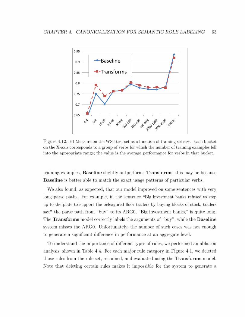
CHAPTER 4. CANONICALIZATION FOR SEMANTIC ROLE LABELING 63
!"#$%
!"&%
!"&$%
!"'%
!"'$%
!"(%
!"($%
!)*%
$)(%
+!)+(%
,!)*(%
$!)((%
+!!)+((%
,!!)*((%
$!!)(((%
+!!!)+(((%
,!!!)*(((%
$!!!-%
./012341%
56/4078690%
Figure 4.12: F1 Measure on the WSJ test set as a function of training set size. Each bucketon the X-axis corresponds to a group of verbs for which the number of training examples fellinto the appropriate range; the value is the average performance for verbs in that bucket.
training examples, Baseline slightly outperforms Transforms; this may be because
Baseline is better able to match the exact usage patterns of particular verbs.
We also found, as expected, that our model improved on some sentences with very
long parse paths. For example, in the sentence “Big investment banks refused to step
up to the plate to support the beleagured floor traders by buying blocks of stock, traders
say,” the parse path from “buy” to its ARG0, “Big investment banks,” is quite long.
The Transforms model correctly labels the arguments of “buy”, while the Baseline
system misses the ARG0. Unfortunately, the number of such cases was not enough
to generate a significant difference in performance at an aggregate level.
To understand the importance of different types of rules, we performed an ablation
analysis, shown in Table 4.4. For each major rule category in Figure 4.1, we deleted
those rules from the rule set, retrained, and evaluated using the Transforms model.
Note that deleting certain rules makes it impossible for the system to generate a

CHAPTER 4. CANONICALIZATION FOR SEMANTIC ROLE LABELING 64
Deleted Rule Group Transforms CombinedNone 88.24 88.47Verb Raising/Control (all) −1.65 −0.54Verb Raising/Control (basic) −1.44 −0.38Verb Raising/Control (nonbasic) −0.12 −0.06Inverted Sentences/Questions +0.10 −0.01“Make” Rewrites −0.44 −0.38Modified Nouns −1.12 −0.38Passive −0.31 −0.36Possessive −0.06 −0.02
Table 4.4: F1 Measure on WSJ test set of Transforms and Combined deletingdifferent subsets of the rules
correct canonical form, guaranteeing failure for some arguments. To avoid parse-
related issues, we trained and evaluated on gold-standard parses. Most important
were rules relating to (basic) verb raising/control and modified nouns; passive and
“make” rewrites were moderately important; and the removal of (nonbasic) verb
raising/control, possessive, and inverted sentences/questions had little or no effect.
More than anything, this indicates the relative frequency of each of these types of
construction.
To get an idea of what areas our system improved over Baseline, we performed the
same ablation analysis on Combined, also shown in Table 4.4. In this case, if the
canonical form system does not include a constituent in the predicted canonical form,
then Baseline is used instead. As expected, the drop in performance from removing,
for example, verb raising/control (basic) is not as large. However, removing each of
verb raising/control (basic), “make” rewrites, modified nouns, and passive rules leads
to a noticeable drop in performance (about 0.4 F1 points in each case).

CHAPTER 4. CANONICALIZATION FOR SEMANTIC ROLE LABELING 65
4.9 Discussion and Future Work
Besides incorporating the ideas used in the state-of-the-art SRL systems described
in Chapter 3, our models could be improved in a variety of ways. One is to im-
prove the coverage of the rule set, adding additional syntactic constructs that are
not already covered. Another is to refine the currently existing rules, with the goal
of incorporating additional features of the rules in order to improve canonical form
selection. For example, our current system does not incorporate lexical features of
the rules. Another related extension would be to add further sentence normaliza-
tions, e.g., identifying whether a direct object exists. We could also add support for
non-core arguments (e.g., temporal arguments).
Another limitation of our current model is that each target verb in a sentence is
labeled separately. This allows the system to produce inconsistent labelings. For
example, in “I want Bob to start to eat,” our system could decide that “I” is the
subject of “start” and that “Bob” is the subject of “eat.” Clearly, both “start” and
“eat” should have the same subject.
As mentioned before, a sentence cannot be labeled entirely correctly unless the
correct role pattern has been seen before; this could be fixed by better modeling of
role patterns. For example, we could find clusters of verbs with similar role patterns,
which would allow us to predict role patterns we have not seen yet.
Another interesting extension involves incorporating parser uncertainty into the
model; in particular, our simplification system is capable of seamlessly accepting a
parse forest as input. The main difficulty is pruning the parse forest in order to
maintain efficiency. With this setup, the parser and simplification system could be
jointly, discriminatively trained to maximize, for example, SRL performance.
The ideas in this chapter can be extended beyond the task of semantic role labeling.
We could augment the system to further normalize canonical forms. For example,
we could map similar verbs to a common frame and rewrite noun phrases containing
nominalizations as verb phrases. Each new type of normalization (assuming it can be
performed accurately) should lead to improvements in higher-level tasks. The primary

CHAPTER 4. CANONICALIZATION FOR SEMANTIC ROLE LABELING 66
difficulty here is the lack of labeled data for further normalizations; this could perhaps
be addressed in the same way as in this chapter, by treating the correct normalized
form as a hidden variable.

Chapter 5
Learning with Contrastive
Objectives
5.1 Introduction
At the end of Chapter 4, we suggested a number of extensions to our canonical SRL
system. Several of these, particularly the suggestion to perform joint inference over all
verbs in the sentence at once, greatly expand the required computation. It is unlikely
that exact inference is tractable in this case, so we need to turn to approximate
learning.
A syntactic parse is a fairly complex object, which makes many existing approaches
to approximate learning difficult to implement. One general class of methods which is
relatively easy to use even for complex objects is heuristic search, where we try to find
a high-scoring configuration by taking a series of steps designed to (sooner or later)
move towards higher-scoring values. Heuristic search is really just an approximate
MAP procedure; unfortunately, previous work has not provided a good way to use
approximate MAP solutions for learning log-linear models. In this chapter, we develop
such a method. Due to additional complications in the canonical SRL model (in
particular, the inclusion of hidden variables), we do not close the loop and apply
these methods to semantic role labeling; instead, we evaluate our method on another
67

CHAPTER 5. LEARNING WITH CONTRASTIVE OBJECTIVES 68
important problem, multiclass image segmentation in real-world images.
5.2 Overview
In Chapter 2, we discussed how learning log-linear models is difficult because of
the complexity of computing the partition function Z(x). Recently there has been
significant interest in contrastive methods such as pseudo-likelihood (PL) (Besag,
1975) and contrastive divergence (CD) (Hinton, 2002). The main idea of these
algorithms is to trade off the probability of the correct assignment for each labeled
example with the probabilities of other, “nearby” assignments. This means that
these algorithms do not need to compute the partition function Z(x). Unfortunately,
these algorithms can suffer when the distribution is highly multi-modal, with multiple
distant regions of high probability.
LeCun & Huang (2005), Smith & Eisner (2005), and Liang & Jordan (2008) all con-
sider the general case of contrastive objectives, where the contrasting set is allowed to
consist of arbitrary assignments. However, previous work has not pursued the idea of
non-local contrastive objectives. Rather than restrict the objective to considering as-
signments (values of Y) that are close to the correct label, as in pseudo-likelihood and
contrastive divergence, we propose methods that allow comparison to any assignment.
This chapter has two main parts. First, we prove several results that justify the
use of non-local contrastive objectives. We show that a wide class of contrastive ob-
jectives are consistent with maximum likelihood, even for finite data under certain
conditions. This generalizes and is a considerably stronger result than the asymptotic
consistency of pseudo-likelihood. A central idea of this result is that contrastive objec-
tives attempt to enforce probability-ratio constraints between different assignments,
based on the structure of the objective. Among other consequences, this result clearly
points out cases in which pseudo-likelihood (and other local methods) may fail.
Based on this insight, we propose several methods for constructing non-local con-
trastive objectives. We focus particularly on Contrastive Constraint Generation
(CCG), a novel constraint-generation style algorithm that iteratively constructs a

CHAPTER 5. LEARNING WITH CONTRASTIVE OBJECTIVES 69
contrastive objective based only on a MAP-inference procedure. While similar in
flavor to the max-margin cutting plane algorithm suggested by Tsochantaridis et al.
(2005), our method has the ability to obtain accurate probability estimates. We
compare CCG to pseudo-likelihood, contrastive divergence, and the cutting-plane al-
gorithm on a real-world machine vision problem; CCG achieves a 12% error reduction
over the best of these, a statistically significant improvement.
5.3 Contrastive Objectives
5.3.1 Definitions
The main idea of our approach is to define small terms over subsets of Y.
Definition 1. Let Sj be some subset of values of Y. The (conditional) contrastive
probability distribution for Sj is Pθ,j(y|x) = eθT f(x,y)
Zj(x), where Zj is the contrastive
partition function Zj(x) =∑
y∈SjeθT f(x,y).
We refer to this distribution as contrastive because it compares the (unnormalized)
probabilities of the values of Y in Sj. Note that this distribution implicitly compares
normalized probabilities: eθT f(x,y)
Zj(x)= Pθ(y|x)P
y′∈SjPθ(y′|x)
due to cancellation of the global
partition function.
Definition 2. A contrastive sub-objective Cj(θ; D) is a weighted maximum-likelihood
objective with the model distribution Pθ replaced by the contrastive distribution Pθ,j
for some subset Sj: ∑(xi,yi):yi∈Sj
wj(xi)(θT f(xi,yi)− log Zj(x
i)).
wj(x) is a parameter of the sub-objective that determines the overall strength of the
sub-objective as well as the relative importance of each value of x.
A contrastive objective C(θ; D) is a sum of J sub-objectives Cj, each with a different
subset Sj and set of weights wj(x). C is tractable to compute (and optimize) if

CHAPTER 5. LEARNING WITH CONTRASTIVE OBJECTIVES 70
the contrastive partition functions are tractable to compute. In some cases, we can
compute the contrastive partition function Zj(x) even if Sj contains an exponential
number of values, e.g., using dynamic programming for tractable sub-structures.
We say that sub-objective Cj is active for example (xi,yi) if yi ∈ Sj and wj(xi) > 0.
The number of active sub-objectives for a particular data set D may be much smaller
than the total number of sub-objectives.
For now, we assume that C is given. We will discuss how to construct contrastive
objectives in Sections 5.7 and 5.8.
5.3.2 Relationship to Standard Learning Methods
The log-likelihood objective LL(θ; D) is a contrastive objective with one sub-objective
C1, where S1 contains all values in Y and w1(x) = 1 for all x.
If Y is an MRF (or CRF), contrastive objectives are a generalization of pseudo-
likelihood. To write PL as a contrastive objective, for each l, for every possible
instantiation y−l, we construct one sub-objective Sy−lthat contains exactly the set
of instantiations consistent with y−l, i.e., (y−l, Yl = a) for all a ∈ dom(Yl). All
sub-objective weights wy−l(x) are set to 1. Since a sub-objective Cy−l
is only ac-
tive for examples where yi ∈ Sy−l, it follows that each example participates in n
sub-objectives, where n is the number of variables in the network. This yields the
contrastive objective
∑(xi,yi)
∑l
(θT f(xi,yi)− log
∑a∈dom(Yl)
eθT f(xi,(yi−l,a))
),
which is the definition of pseudo-likelihood. All of the sub-objectives in PL are local ;
they only involve instantiations that differ on a single node. Generalized pseudo-
likelihood (GPL) can also easily be expressed in this framework. In GPL two or more
variables are allowed to vary. This can lead to large, potentially exponential sub-
objectives. In some cases, dynamic programming can render inference tractable within
sub-objectives. Unlike GPL, our framework allows us to vary multiple variables

CHAPTER 5. LEARNING WITH CONTRASTIVE OBJECTIVES 71
without including all possible combinations of these variables, giving us considerably
more flexibility.
Another related learning method is contrastive divergence (CD), which approxi-
mates the gradient of maximum likelihood using a non-mixed Markov chain, initial-
ized at the label of the current example. CD is generally defined by the update
rule
∆θt =∑
(xi,yi)
ft(xi,yi)− EP k
θ(ft(x
i,yi)),
where P kθ is the distribution over y obtained by initializing some Markov chain Monte
Carlo (MCMC) procedure at xi and running for k steps.1 CD cannot be expressed
as a contrastive objective, because CD uses P kθ to compute expectations rather than
Pθ. This means that the probability-ratio matching intuitions in the next section do
not hold for CD. In fact, CD does not optimize any objective. This means that CD
requires using stochastic gradient for optimization, whereas a contrastive objective
can be optimized using a variety of methods (in this paper, BFGS). Furthermore,
similar to PL, standard implementations of CD are local: they compare the correct
label yi only to nearby values y′.
5.3.3 Visualization of Contrastive Objectives
In this section, we present a visualization of contrastive objectives which gives insight
into how they work. Figure 5.1 depicts a probability distribution and an observed
data set. We assume that the probability distribution is the model distribution Pθ
for some parameter vector θ.
Figure 5.2 shows a representation of the gradient of the log-likelihood objective.
The probability of every point is adjusted, with size proportional to how far off the
current model probability is from the observed data distribution. Figure 5.3 shows
the gradient of pseudo-likelihood (assuming that nearby points in the visualization
corresponds to instantiations that differ on a single variable). Only neighboring points
1In practice, it is intractable to compute the expectation over P kθ exactly; instead, it is estimated
through sampling.

CHAPTER 5. LEARNING WITH CONTRASTIVE OBJECTIVES 72
Figure 5.1: Probability distribution andobserved data set. The size of each circlerepresents the probability assigned to thatpoint. Yellow circles are observed data ex-amples; each is observed once, so |D| = 7.
Figure 5.2: Representation of log-likelihoodgradient. A green upward arrow abovea point indicates positive gradient; a reddownward arrow indicates negative gradi-ent. Size of arrow indicates gradient magni-tude. Very small arrows have been omitted.
are compared.
Figure 5.4 shows a single local pairwise sub-objective, which is similar to a reduced
PL sub-objective. Figure 5.5 shows an example of a non-local pairwise sub-objective.
This sub-objective allows us to “fix” the large blue dot at the top of the visualization.
Finally, Figure 5.6 shows a sub-objective that compares points that are already “ok”
(i.e., the labeled point has much higher probability than the unlabeled); the resulting
gradient is small.
5.3.4 Other Related Methods
LeCun & Huang (2005) provide a general framework for learning energy functions
of which contrastive objectives are an example, but do not suggest the particular
log-linear form used in our work. Smith & Eisner (2005) define an objective with the
same functional form as one of our sub-objectives; however, they primarily look at
unsupervised learning tasks, whereas this work is mostly aimed at supervised learning.

CHAPTER 5. LEARNING WITH CONTRASTIVE OBJECTIVES 73
Figure 5.3: Pseudo-likelihood Figure 5.4: Local sub-objective
Figure 5.5: Non-local sub-objective Figure 5.6: “Satisfied” sub-objective
CHAPTER 5. LEARNING WITH CONTRASTIVE OBJECTIVES 74
More importantly, both of these works focus on the use of local contrastive objectives,
whereas we are particularly interested in the use of non-local contrastive terms.
Liang & Jordan (2008) provide an asymptotic analysis of contrastive objectives.
They show that under certain conditions, the more different assignments are covered
by the objective, the more efficient the objective is as an estimator. They apply this
result to compare the efficiency of pseudo-likelihood to that of maximum-likelihood.
Their results suggest that increasing the number of assignments covered by the con-
trastive objective leads to improved learning efficiency.
Hyvarinen (2007) proposes an objective for learning binary Markov networks by
trying to match ratios of probabilities between the model and the observed data.
This objective minimizes squared-loss instead of log-loss; the advantage of log-loss is
that contrastive objectives are a direct generalization of both log-likelihood and PL.
Additionally, Hyvarinen (2007) only proposes matching local probability ratios.
Recently, Gutmann & Hyvarinen (2010) proposed a method based on learning prob-
ability ratios between the data distribution and some hand-constructed noise distri-
bution. Similar to our method, it does not require computation of the global partition
function. Unlike our method, it looks at probability ratios between different distribu-
tions, while our method looks at probability ratios between different instantiations.
Hinton et al. (2004) and Tieleman (2008) both improve CD by adding non-local
contrastive terms. However, like standard CD, these methods do not correspond
to any objective function. The following analysis gives a theoretical grounding to
non-local contrastive learning and supplies a well-defined objective.
Max-margin-based methods, such as those proposed by Taskar et al. (2003) and
Tsochantaridis et al. (2005), also are designed to avoid needing to compute the global
partition function. The cutting-plane algorithm proposed by Tsochantaridis et al.
(2005) is similar in spirit to our contrastive constraint-generation (CCG) approach,
described in Section 5.8. Like max-margin methods, CCG can learn using only MAP
inference. The primary advantage of contrastive objectives over margin-based meth-
ods is that they can calibrate probabilities between instantiations.

CHAPTER 5. LEARNING WITH CONTRASTIVE OBJECTIVES 75
5.4 Theoretical Results
The main results of this section show the finite and asymptotic consistency of con-
trastive objectives, under suitable conditions on the model distribution Pθ and sub-
objectives Cj. The proofs of these theoretical results also illustrate a key feature of
contrastive objectives: if two label values y,y′ are connected through a series of sub-
objectives, then the objective will encourage Pθ(y|x)Pθ(y′|x)
to match P (y|x)
P (y′|x). This will be
the main motivation for the methods we propose in Sections 5.7 and 5.8 for choosing
non-local sub-objectives.
5.4.1 Consistency of Pseudo-likelihood
Before presenting the results, we review asymptotic consistency for pseudo-likelihood.
We begin by establishing some notation.
Let Θ be the set of all possible parameter vectors θ, and let PΘ denote the set of all
possible models Pθ obtainable using θ ∈ Θ. We say that PΘ can represent probability
distribution P ′(Y|X) if there exist parameters θ′ ∈ Θ such that Pθ′(Y|x) = P ′(Y|x)
for all x. Let Θ[P ′] denote the set of such θ′.
Let P ∗(Y,X) be the distribution from which the data set D is drawn. Let {d1, d2, . . . }be an infinite sequence of examples drawn i.i.d from P ∗(X,Y); we refer to the data set
composed of the first n of these as Dn, and its empirical distribution as P (y|x; Dn).
By the strong law of large numbers, P (limn→∞ P (y|x; Dn) = P ∗(X,Y)) = 1, or in
short-hand P converges to P ∗ almost surely P (y|x; Dn)a.s.→ P ∗(y|x) as n→∞.
Gidas (1988) proved consistency of log-likelihood and pseudo-likelihood. The state-
ment of consistency for pseudo-likelihood is the following:
Theorem 1. Suppose PΘ can represent P ∗(Y|X). Also, suppose that for all x such
that P ∗(x) > 0, P ∗(Y|x) is positive, i.e., for all y, P ∗(y|x) > 0. Let θ(n) be a
sequence of weight vectors {θ1, θ2, . . . } such that for all n, θn optimizes PL(θ; Dn).
Then for all x s.t. P ∗(x) > 0, Pθn(Y|x)a.s.→ P ∗(Y|x) as n→∞
This means that, provided the data is drawn from within our model class (and that

CHAPTER 5. LEARNING WITH CONTRASTIVE OBJECTIVES 76
the data distribution is positive), we will converge to the correct parameters as the
amount of data grows. This theorem follows from Theorem 3, proved in Section 5.4.3.
Before proving asymptotic consistency for (a certain class) of contrastive objectives,
we will first consider finite consistency for contrastive objectives.
5.4.2 Finite Consistency
While asymptotic representability (i.e., PΘ being able to represent P ∗(Y|X)) is a
standard concept in analysis of learning algorithms, finite representability (PΘ being
able to represent P (Y|x)) is less common. Suppose PΘ can represent P (Y|x). In
many cases, we only see each X = x one time in our data set D, which means that
P (Y|X) will have a point estimate on the correct label yi for each xi. Thus, it can
be a fairly strong condition on our model class PΘ. However, as we will now show, it
is actually a weaker condition than another commonly seen condition in analysis of
learning algorithms: separability.
Typically it is assumed that Θ is exactly equal to RR (i.e., any possible R-length
vector of real numbers). For the purposes of the following result, we will augment Θ
to also include (a certain type of) infinite-length weight vectors. Specifically, for each
unit vector θ′ ∈ RR, we include an infinite length weight vector θ′∞; the corresponding
model distribution is Pθ′∞(y|x) = limλ→∞ Pλθ′(y|x). We refer to this expanded set as
Θ∞. This augmentation simply adds certain deterministic distributions to PΘ.
A classifier γ is a deterministic function from X to Y. We say that a data set D
is separable with respect to a set of classifiers Γ = {γk} if there exists some classifier
γk ∈ Γ such that γk(xi) = yi for all data instances di in D.
Lemma 1. Let ΓΘ be the set of classifiers γθ such that γθ(x) = arg maxy Pθ(y|x) (if
the arg max is not unique, γθ(x) is undefined and so cannot separate with respect to
x). If D is separable with respect to ΓΘ, then PΘ∞ can represent P (Y|X).
Proof. Since D is separable with respect to ΓΘ, there exists a classifier γθ such that
arg maxy Pθ(y|xi) = yi for all data instances di. Let θλ = λθ. Then Pθλ(yi|xi) =

CHAPTER 5. LEARNING WITH CONTRASTIVE OBJECTIVES 77
eλθT f(xi,yi)Py eλθT f(xi,y)
= 1
1+eλP
y 6=yi eθT f(xi,y)−θT f(xi,yi). But in this last expression, all exponents
are negative since yi = arg maxy Pθ(y|xi) = arg maxy θT f(xi,y). Thus, as λ → ∞,
Pθλconverges to a point estimate on the observed label value yi given each xi. But
since D is separable, it must be that P consists of the same point estimates, and so
limλ→∞ Pθλ= P . But if θ∞ is the infinite length weight vector in the direction of θ,
this means that Pθ∞ = P .
There are a couple of things to note about this result. First, the set of classifiers ΓΘ
is precisely the set of linear separators of the form θT f(X,Y), a well-studied set of
classifiers (and with which the notion of separability is often used). Second, although
we needed to use an infinite-length weight vector to exactly represent P , if the data is
separable, then we can obtain an arbitrarily close approximate to P using finite-length
weight vectors. We will assume exact representability for the remainder of this section,
but replacing with “near-exact” representability would only slightly weaken the results
(specifically, it would add an arbitrarily small approximation factor). Finally, note
that the converse does not hold: there are data sets D such that P is representable
by PΘ∞ but which are not separable (either by ΓΘ or by any other set of classifiers).
Trivially, any D such that yi is not deterministic given xi is not separable but may
still be representable.
Let Pj be the contrastive observed data distribution restricted to Sj: Pj(y|x) =|(xi,yi)=(x,y)|
Zj(x)= P (x,y)P
y∈SjP (x,y)
where Zj(x) = |(xi,yi) : xi = x and y ∈ Sj|.
It will be convenient to define a slightly modified version C ′(θ; D) of our contrastive
objective:
−∑
j
∑(xi,yi):yi∈Sj
wj(xi) ∗ (log
eθT f(xi,yi)
Zj(xi)− log Pj(y
i|xi)).
By definition, C ′(θ; D) differs from C(θ; D) only by flipping the sign and adding a
constant; thus the maxima of C(θ; D) are the same as the minima of C ′(θ; D). For

CHAPTER 5. LEARNING WITH CONTRASTIVE OBJECTIVES 78
the remainder of this section, we will analyze C ′(θ; D). Rewriting C ′(θ; D), we get
∑j,x
P (x)wj(x)∑y∈Sj
P (y|x)(log Pj(y|x)− log Pθ,j(y|x))
=∑j,x
P (x)wj(x)Zj(x)
Z(x)
∑y∈Sj
Pj(y|x) logPj(y|x)
Pθ,j(y|x)
=∑j,x
P (x)wj(x)(∑y∈Sj
P (y|x))KL(Pj(y|x)||Pθ,j(y|x))
Thus, C ′(θ; D) is a weighted linear combination of KL-divergences.
Lemma 2. Suppose that PΘ can represent P (y|x). Then for any contrastive objective
C ′(θ; D),
i. For any θ ∈ Θ[P ], C ′(θ; D) has a global optimum at θ, with C ′(θ; D) = 0.
ii. If θ′ optimizes C ′(θ; D), then for any j,x such that P (x)wj(x)(∑
y∈SjP (y|x)) >
0, we have Pθ′,j(y|x) = Pj(y|x).
Proof. To prove (i), let θ ∈ Θ[P ]. Then
Pθ,j(y|x) = Pθ(y|x)Py′∈Sj
Pθ(y′|x)= P (x,y)P
y∈SjP (x,y)
= Pj(y|x).
Thus, for all j,x, KL(Pj(y|x)||Pθ,j(y|x)) = 0, and so C ′(θ; D) = 0. Since C ′(θ; D)
is a weighted linear combination of KL-divergences, it is non-positive for all θ, and
so θ is a global optimum of C ′(θ; D).
To prove (ii), suppose θ′ optimizes C ′(θ; D). From (i), it follows that C ′(θ′; D) = 0.
Now, since each C ′j(θ; D) is non-negative, if C ′(θ′; D) = 0, then C ′
j(θ′; D) = 0 for all j.
If wj(x) > 0 and∑
y∈SjP (x,y) > 0, then KL(Pj(y|x)||Pθ,j(y|x)) has a positive coef-
ficient in C ′j(θ; D); since KL is non-negative, it follows that KL(Pj(y|x)||Pθ′,j(y|x)) =
0.
Corollary 1. Suppose that PΘ can represent P (y|x) and θ′ optimizes C ′(θ; D). Also
suppose y1,y2 ∈ Sj, P (x) > 0, P (y1|x) > 0, and wj(x) > 0. ThenPθ′ (y2|x)
Pθ′ (y1|x)= P (y2|x)
P (y1|x).

CHAPTER 5. LEARNING WITH CONTRASTIVE OBJECTIVES 79
Proof. The stated conditions ensure that the premises of Lemma 2 part (ii) hold.
Thus, Pθ′,j(y|x) = Pj(y|x). But P (y2|x)
P (y1|x)=
Pj(y2|x)
Pj(y1|x)and
Pθ′,j(y2|x)
Pθ′,j(y1|x)=
Pθ′ (y2|x)
Pθ′ (y1|x)due to
cancellation of partition functions, and we are done.
Thus, the probability ratios according to Pθ′ match those according to P within a
sub-objective set.
Definition 3. We are given a set of sub-objectives Cj with weights wj(x). For a
fixed feature value x, we say that there is a path from y1 to y2 relative to probability
distribution P (Y|x) if there is a sequence Sjb: b = 1, ..., k such that
i. y1 ∈ Sj1 and y2 ∈ Sjk
ii. for every consecutive pair Sjb, Sjb+1
, there exists zb ∈ dom(Y) s.t. zb ∈ Sjb,
zb ∈ Sjb+1, and P (zb|x) > 0
iii. wjb(x) > 0 for all jb
Intuitively, this definition means that it is possible to “walk” from y1 to y2: if you
are currently at value y, you are allowed to move to any other value y′ if y and
y′ both are contained in some sub-objective set Sj with positive weight wj(x). If
P (y′|x) = 0, the walk must stop; otherwise it can continue.
Lemma 3. Suppose that PΘ can represent P (y|x) and θ′ optimizes C ′(θ; D). Also,
suppose that P (x) > 0, P (y1|x) > 0, and there is a path from y1 to y2 relative to
P (Y|x). ThenPθ′ (y2|x)
Pθ′ (y1|x)= P (y2|x)
P (y1|x).
Proof. By definition of path, there exists a sequence Sjbsuch that y1 ∈ Sj1 , y2 ∈ Sjk
,
wjb(x) > 0, and for every consecutive pair Sjb
, Sjb+1, there exists a zb such that
zb ∈ Sjb, zb ∈ Sjb+1
, and P (zb) > 0. This definition guarantees that the conditions of
Corollary 1 hold for each sub-objective Cjb(note that for Cj1 , both P (y1|x) > 0 and
P (z1|x) > 0). It immediately follows that

CHAPTER 5. LEARNING WITH CONTRASTIVE OBJECTIVES 80
P (y2|x)
P (y1|x)=
P (z1|x)
P (y1|x)∗ P (z2|x)
P (z1|x)· · · ∗ P (y2|x)
P (zk−1|x)
=Pθ′(z1|x)
Pθ′(y1|x)∗ Pθ′(z2|x)
Pθ′(z1|x)· · · ∗ Pθ′(y2|x)
Pθ′(zk−1|x)
=Pθ′(y2|x)
Pθ′(y1|x)
We now have that the probability ratios according to Pθ′(y|x) match those accord-
ing to P (y|x) for any pair of values y1,y2 connected by a path (relative to P (Y|x)).
Definition 4. For fixed x, a set of sub-objectives Sj with weights wj(x) span Y
relative to a probability distribution P (Y|x) if for every pair of values y1,y2 there is
a path from y1 to y2 relative to P (Y|x).
Note that this condition requires the total size of our sub-objectives to be at least
the cardinality of Y.
Let Θ′ be the set of θ′ that optimize C ′(θ; D).
Theorem 2. Suppose that PΘ can represent P (y|x). Furthermore, suppose that for
every xi (i.e., every value of X observed in D), our sub-objectives Sj with weights
wj(xi) span Y relative to P (Y|xi). Then Θ′ = Θ[P ]. That is, θ′ optimizes C ′(θ; D)
if and only if Pθ′(Y|xi) = P (Y|xi) for all xi.
Proof. From Lemma 2, Θ[P ] ⊆ Θ′. We need to show that under the given conditions
on C ′(θ; D), Θ′ ⊆ Θ[P ].
Let x be any feature value that occurs in D. Then P (x) > 0. Choose some y1 such
that P (y1|x) > 0. By the definition of span, for every other value y2, there exists a
path from y1 to y2 relative to P (Y|x). From Lemma 3,Pθ′ (y2|x)
Pθ′ (y1|x)= P (y2|x)
P (y1|x).
Suppose θ′ optimizes C ′(θ; D). Then for all y2, Pθ′(y2|x) =Pθ′ (y1|x)
P (y1|x)∗ P (y2|x). But
Pθ′ (y1|x)
P (y1|x)is simply some constant, and so Pθ′ and P differ only by a multiplicative

CHAPTER 5. LEARNING WITH CONTRASTIVE OBJECTIVES 81
factor. But this immediately implies that they are the same distribution, Pθ′(y|x) =
P (y|x). Thus θ′ ∈ Θ[P ] and Θ′ ⊆ Θ[P ].
The optima of the log-likelihood objective are exactly Θ[P ] (provided PΘ can rep-
resent P (y|x)). Thus, the optima of any contrastive objective fulfilling the conditions
of the previous theorem are exactly the same as those of the log-likelihood objective.
5.4.3 Asymptotic Consistency
We will now extend the previous results to the case of infinite data. With the ex-
ception of Lemma 4, the proofs of all results in this section closely mirror the corre-
sponding results from the previous section.
As before, let {d1, d2, . . . } be an infinite sequence of examples drawn i.i.d from
P ∗(X,Y), with Dn and P (y|x; Dn) defined as before. Let θ(n) be a sequence of
weight vectors {θ1, θ2, . . . } such that for all n, θn optimizes C ′(θ; Dn).
Lemma 4. Suppose that PΘ can represent P ∗(y|x). Then for any contrastive objec-
tive C ′,
i. For any θ∗ ∈ Θ[P ∗], C ′(θ∗; Dn)a.s.→ 0 as n→∞.
ii. For any θ(n) defined as above, for any j,x such that P ∗(x)wj(x)(∑
y∈SjP ∗(y|x)) >
0, Pθn,j(y|x)a.s.→ P ∗
j (y|x) as n→∞.
Proof. As noted above, P (y|x; Dn)a.s.→ P ∗(y|x) as n→∞. This means that for θ∗ ∈
Θ[P ∗], KL(Pj(y|x; Dn)||Pθ∗,j(y|x))a.s.→ 0 as n → ∞ for all j. Thus C ′(θ∗; Dn)
a.s.→ 0
as n→∞.
Now we prove (ii). From part (i), C ′(θ∗; Dn)a.s.→ 0 as n→∞. But since θn optimizes
C ′(θ; Dn), C ′(θn; Dn) ≤ C ′(θ∗; Dn) for all n. This implies that C ′(θn; Dn)a.s.→ 0 as
n→∞.
Since P (y|x; Dn)a.s.→ P ∗(y|x) as n→∞, it follows that there is some N such that for
all n ≥ N , P (y|x; Dn) > 0 if and only if P ∗(y|x) > 0. Thus, if wj(x)∑
y∈SjP ∗(x,y) >
0, then it is also the case that wj(x)∑
y∈SjP (x,y; Dn) > 0 for n ≥ N . This means

CHAPTER 5. LEARNING WITH CONTRASTIVE OBJECTIVES 82
that for sufficiently large n, if wj(x)∑
y∈SjP ∗(x,y) > 0, then KL(Pj(y|x; Dn)||Pθ,j(y|x))
has a positive coefficient in C ′j(θ; Dn).
Putting the previous two paragraphs together, KL(Pj(y|x; Dn)||Pθn,j(y|x))a.s.→ 0
as n→∞. But this implies Pθn,j(y|x)a.s.→ P ∗
j (y|x) as n→∞ and we are done.
Corollary 2. Suppose that PΘ can represent P ∗(y|x). Also suppose y1,y2 ∈ Sj,
P ∗(x) > 0, P ∗(y1|x) > 0, and wj(x) > 0. Then for any θ(n), Pθn (y2|x)Pθn (y1|x)
a.s.→ P ∗(y2|x)P ∗(y1|x)
as
n→∞.
Lemma 5. Suppose that PΘ can represent P ∗(y|x). Also, suppose that P ∗(x) > 0,
P ∗(y1|x) > 0, and there is a path from y1 to y2 relative to P ∗(Y|x). Then for any
θ(n), Pθn (y2|x)Pθn (y1|x)
a.s.→ P ∗(y2|x)P ∗(y1|x)
as n→∞.
Finally, we can prove full asymptotic consistency:
Theorem 3. Suppose that PΘ can represent P ∗(y|x). Furthermore, suppose that for
every x such that P ∗(x) > 0, our sub-objectives Sj with weights wj(x) span Y relative
to P ∗(Y|x). Then for any θ(n) and any x such that P ∗(x) > 0, Pθn(Y|x)a.s.→ P ∗(Y|x)
as n→∞.
Proof. Let x be any feature value such that P ∗(x) > 0. Choose some y1 such that
P ∗(y1|x) > 0. From Lemma 5, for all other y2,Pθn (y2|x)Pθn (y1|x)
a.s.→ P ∗(y2|x)P ∗(y1|x)
as n→∞. From
here it is a technical exercise to show that Pθn(Y|x)a.s.→ P ∗(Y|x) as n→∞, and we
are done.
From this result we can derive consistency of pseudo-likelihood for strictly positive
data distributions Pθ∗ (i.e., Pθ∗(y|x) > 0 for all y,x), simply by noting that in the
limit of infinite data, the set of active PL sub-objectives will span Y. It is also easy
to see why PL is usually not consistent with finite data (it is unlikely to span the
space), and why it may not be consistent for non-positive data distributions (again,
because it may not span the space).
The most important practical implication from this section is that a contrastive
objective attempts to calibrate probabilities within connected components of sub-
objectives but cannot calibrate probabilities between disconnected components. This

CHAPTER 5. LEARNING WITH CONTRASTIVE OBJECTIVES 83
has important implications for the performance of PL (and other local contrastive
objectives), as we will see in Section 5.9.
5.5 Weight Decomposition
So far we have not examined the effect of the choice of weights wj(x) beyond whether
wj(x) > 0. In order to better understand the effect of the weights on the ob-
jective, we will rewrite the weights as a product of three terms, wj(x) = w(x) ∗∑y P (Cj|y,x)Q(y|x), each of which is chosen by the designer of the contrastive ob-
jective.
The first term w(x) allows the designer to reweight the relative importance of
terms in the objective corresponding to different values of x. This could be useful if
we believe that the empirical distribution P (x) observed in our data does not match
the true (or desired) distribution over x (in general, we assume that P (y|x) must be
drawn from the true underlying distribution, but this may or may not be the case
for P (x)). These weights can also be used in standard maximum likelihood training
and are related to work in the area of domain adaptation (see, for example, (Mansour
et al., 2009)). We will not focus on this part of the weights in this paper, assuming
that they are uniform across all x. The second term P (Cj|y,x) allows the designer
to choose the relative importance of different sub-objectives for a particular value of
the label variable y (and also relative to a feature value x). P (Cj|y,x) is constrained
to be a probability distribution such that P (Cj|y,x) > 0 only when y ∈ Sj. The
third term Q(y|x) is an auxiliary probability distribution that allows the designer to
choose how important each y is to the objective.
Putting these terms together, wj(x) = w(x)∗∑
y P (Cj|y,x)∗Q(y|x). Since P and
Q are both probability distributions, the sum of all weights wj(x) for a given x is
w(x). This means that P and Q do not affect the relative influence of different values
of x. This decomposition of the weights wj(x) is over-parametrized; in particular, it
is not hard to show that we can write any choice of wj(x) in this form. Specifically,
let w(x) =∑
j wj(x), and define P ′(Cj|x) =wj(x)Pj wj(x)
. We now simply need to choose
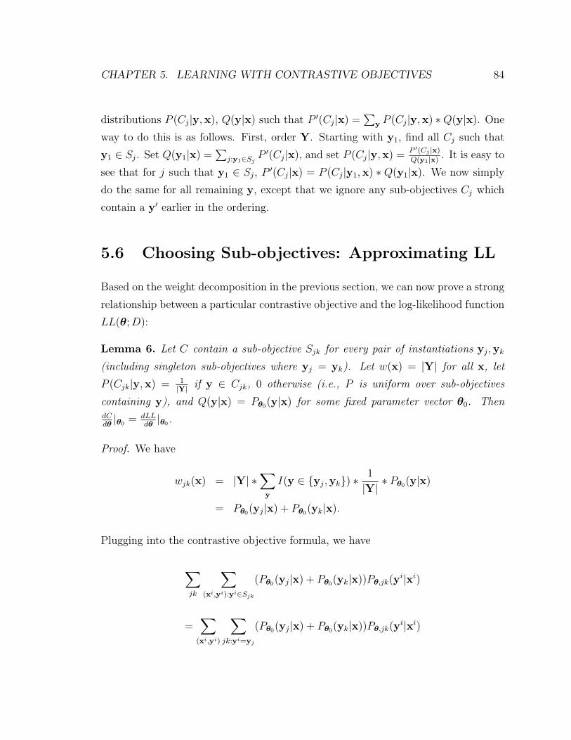
CHAPTER 5. LEARNING WITH CONTRASTIVE OBJECTIVES 84
distributions P (Cj|y,x), Q(y|x) such that P ′(Cj|x) =∑
y P (Cj|y,x) ∗Q(y|x). One
way to do this is as follows. First, order Y. Starting with y1, find all Cj such that
y1 ∈ Sj. Set Q(y1|x) =∑
j:y1∈SjP ′(Cj|x), and set P (Cj|y,x) =
P ′(Cj |x)
Q(y1|x). It is easy to
see that for j such that y1 ∈ Sj, P ′(Cj|x) = P (Cj|y1,x) ∗ Q(y1|x). We now simply
do the same for all remaining y, except that we ignore any sub-objectives Cj which
contain a y′ earlier in the ordering.
5.6 Choosing Sub-objectives: Approximating LL
Based on the weight decomposition in the previous section, we can now prove a strong
relationship between a particular contrastive objective and the log-likelihood function
LL(θ; D):
Lemma 6. Let C contain a sub-objective Sjk for every pair of instantiations yj,yk
(including singleton sub-objectives where yj = yk). Let w(x) = |Y| for all x, let
P (Cjk|y,x) = 1|Y| if y ∈ Cjk, 0 otherwise (i.e., P is uniform over sub-objectives
containing y), and Q(y|x) = Pθ0(y|x) for some fixed parameter vector θ0. ThendCdθ|θ0 = dLL
dθ|θ0.
Proof. We have
wjk(x) = |Y| ∗∑y
I(y ∈ {yj,yk}) ∗1
|Y|∗ Pθ0(y|x)
= Pθ0(yj|x) + Pθ0(yk|x).
Plugging into the contrastive objective formula, we have
∑jk
∑(xi,yi):yi∈Sjk
(Pθ0(yj|x) + Pθ0(yk|x))Pθ,jk(yi|xi)
=∑
(xi,yi)
∑jk:yi=yj
(Pθ0(yj|x) + Pθ0(yk|x))Pθ,jk(yi|xi)

CHAPTER 5. LEARNING WITH CONTRASTIVE OBJECTIVES 85
Taking the derivative with respect to some parameter θl, we have
∑(xi,yi)
∑jk:yi=yj
(Pθ0(yj|xi) + Pθ0(yk|xi)) ∗0@fl(x
i,yi)−fl(x
i,yj)eθT f(xi,yj)
+fl(xi,yk)eθT f(xi,yk)
eθT f(xi,yj)
+eθT f(xi,yk)
1A=∑
(xi,yi)
∑jk:yi=yj
(Pθ0(yj|xi) + Pθ0(yk|xi)) ∗„
fl(xi,yi)−
fl(xi,yj)Pθ(yj |x
i)+fl(xi,yk)Pθ(yk|x
i)
Pθ(yj |xi)+Pθ(yk|xi)
«.
Evaluating at θ = θ0 and multiplying through, we get
∑(xi,yi)
∑jk:yi=yj
(fl(xi,yi)Pθ0(yj|xi) + fl(x
i,yi)Pθ0(yk|xi)
− fl(xi,yj)Pθ0(yj|xi)− fl(x
i,yk)Pθ0(yk|xi))
But since yj = yi in the summation, we can cancel to get
∑(xi,yi)
∑k
(fl(x
i,yi)Pθ0(yk|xi)− fl(xi,yk)Pθ0(yk|xi)
)=∑
(xi,yi)
(fl(x
i,yi)∑
k
Pθ0(yk|xi)−∑
k
fl(xi,yk)Pθ0(yk|xi)
)
=∑
(xi,yi)
(fl(x
i,yi)−∑
k
fl(xi,yk)Pθ0(yk|xi)
).
But this is exactly the derivative of LL at θ0 (observed minus expected).
Thus, at any point θ in weight space, we can construct a contrastive objective
tangent to log-likelihood at θ. As a result, we can optimize LL using an EM-like
algorithm. We initialize with weight vector θ0. During the ith Expectation step, we
update Q(y|x) = Pθi−1(y|x). During the ith Maximization step, we fix Q and use
C to compute the gradient of log-likelihood at θi−1. We then take a step in the
CHAPTER 5. LEARNING WITH CONTRASTIVE OBJECTIVES 86
direction of the gradient, obtaining a new weight vector θi. This algorithm has some
similarities to an algorithm proposed by Hoefling & Tibshirani (2009) for optimizing
log-likelihood using a series of pseudo-likelihoods. Significant differences are that
our algorithm is more general, using any contrastive objective; and our method uses
approximations that are within the parametric family of contrastive objectives, while
the method proposed by Hoefling & Tibshirani (2009) approximates using a modified
PL term.
There are several limitations on the practical use of this result. First, computing
the auxiliary distribution Q requires computing the global partition function Zθ0(x).
There is a workaround, however: in addition to setting Q(y|x) = Pθ0(y|x), we also
(implicitly) set w(x) = |Y| ∗ Zθ0(x). The resulting weight wjk(x) = (|Y| ∗ Zθ0(x)) ∗∑y∈Cjk
1|Y| ∗ Pθ0(y|x) = Zθ0 ∗ (Pθ0(yj|x) + Pθ0(yk|x) = eθT
0 f(yj ,x) + eθT0 f(yk,x). This
final expression is simply the exponentiated scores of two different examples, so it is
easy to compute. The cost of this modification is that we have affected the relative
importance of different values of x in the contrastive objective C. If x is empty
(e.g., we are working with an unconditioned Markov network), this does not affect
the objective at all (beyond a multiplicative rescaling). For the general case, this will
only be a problem if Zθ0(x) varies wildly for different x; even in this case, since the
effect of the partition function is less direct than in maximum likelihood, we might
expect approximation schemes for Zθ0(x) to work well.
A second limitation is that exact computation of the gradient still requires an
exponential number of sub-objectives. However, this way of looking at computing
the gradient may lead to new approximation schemes for optimizing LL.
5.7 Choosing Sub-objectives: Fixed Methods
In practice we are not going to be able to span Y with our sub-objectives. An
obvious approximation is to drop sub-objectives. The effect of this will be to partition
the domain of Y; within each connected component the objective will attempt to
calibrate probabilities, but probabilities will not be calibrated across components. In

CHAPTER 5. LEARNING WITH CONTRASTIVE OBJECTIVES 87
Figure 5.7: Estimate of λ0 (y-axis) vs. λ1 used to generate the data (x-axis). The plot showsmedian learned parameter value over 100 synthetic data sets, each with 1000 instances.Error bars indicate 25th and 75th percentile estimates. Correct λ0 = .139. Error bars forPL extend off graph for large λ1.
this section, we propose several techniques for constructing tractable objectives and
examine some of their properties. The methods discussed in this chapter are fixed
— a single contrastive objective is constructed and optimized. In Section 5.8, we
will explore an iterative method, in which the contrastive objective changes as the
algorithm runs.
5.7.1 Simple Fixed Methods
One obvious method for constructing sub-objectives is to use expert knowledge to
determine useful values to compare. In pseudo-likelihood, for example, each sub-
objective corresponds to instantiations that differ on a (particular) single variable.
In generalized PL, sub-objectives contain all instantiations that differ on a particular
subset of variables.
As a concrete example of a sub-objective that is not possible using (generalized) PL,
we consider a binary chain MRF consisting of 10 nodes. The model is unconditional
(i.e., x is empty), and it has only two parameters: a single bias term specifying the
relative weight of 0 vs. 1; and a single affinity term that specifies how likely two

CHAPTER 5. LEARNING WITH CONTRASTIVE OBJECTIVES 88
neighboring nodes are to have the same value. Thus, the log-score of an instantiation
is λ0 ∗ |yi = 1| + λ1 ∗ |yi = yi+1|. For large λ1, the instantiations {000000000} and
{1111111111} have much higher probability than any other instantiations; thus, we
expect PL to have trouble fitting λ0 in this case, since it does not directly compare
the probabilities of these two instantiations. However, we can easily augment the
PL objective with an additional sub-objective containing exactly these two values —
we refer to this objective as Simple Contrastive. Figure 5.7 shows the error in the
estimate of λ0 as we vary the affinity parameter λ1. Simple Contrastive is able to
accurately reconstruct λ0 for all values of λ1, while PL is not. Contrastive objectives
constructed in this way can be quite powerful but are somewhat difficult to design.
We discuss this issue further in Section 5.7.3.
A different kind of approach is to use the data D to guide the selection of sub-
objectives. For unconditioned Markov networks, a simple approach is to construct
sub-objectives that compare different observed values of the label variables yi. This
ensures that far-apart instantiations are compared (assuming that the data contains
such instantiations). We employed this strategy for the MRF described above, aug-
menting PL with a single sub-objective containing all values observed in D. This
objective is referred to as Contrastive. As shown in Figure 5.7, Contrastive is also
effective at recovering λ0, although for low values of λ1, the estimate is slightly inac-
curate. We discuss this further in the next section.
5.7.2 Bias
In the previous section, we made a distinction between methods that choose sub-
objectives ahead of time and those that choose sub-objectives using D. We now
formalize this idea and briefly discuss the differences between the two methods.
A method for choosing sub-objectives is data-independent if the weights wj(x) do
not depend on D. Put another way, wj(x) must be the same regardless of the ex-
amples observed in D. A method is data-dependent if it is not data-independent.
Constructing a useful data-independent contrastive objective is generally more diffi-
cult than constructing a data-dependent objective, but data-independent objectives

CHAPTER 5. LEARNING WITH CONTRASTIVE OBJECTIVES 89
have a significant advantage:
Lemma 7. Suppose that wj(x) does not depend on D. Then EP ∗ [dC(θ;D)dθ|θ0 ] =
dC(θ;D∗)dθ
|θ0 for all θ0, where D∗ is a data set (of possibly infinite size) such that
P (y|x; D∗) = P ∗(y|x).
Proof. Taking the derivative of C(θ; D) with respect to parameter θl and plugging in
θ0, we get
∑j
∑(xi,yi):yi∈Sj
wj(xi) ∗ (fl(x
i,yi)− EPθ0,j(y|xi)[fl(xi,y)])
=∑j,x
wj(x)∑y∈Sj
P (x,y)(fl(x,y)− EPθ0,j(y|x)[fl(x,y)])
The only term in the expression that depends on D is P (x,y). Thus, by linearity
of expectation, we have that EP ∗ [dC(θ;D)dθ|θ0 ] is equal to
∑j,x
wj(x)∑y∈Sj
EP ∗ [P (x,y)](fl(x,y)− EPθ0,j(y|x)[fl(x,y)]).
But EP ∗ [P (x,y)] = P ∗(x,y), and we are done. If the objective data-dependent
(i.e., wj(x) depends on D), then we can no longer push the expectation inside of the
summations, and in general the equality no longer holds.
This lemma shows that for a data-independent method, we get an unbiased estimate
of the gradient at any point θ0. Suppose that PΘ can represent P ∗(y|x). In this case,
we can apply this lemma at θ0 = θ∗ to get that the expectation D of the gradient
at θ∗ is 0. Loosely speaking, this means that the learned parameters for different
D sampled from P ∗ will be centered around θ∗. Data-dependent methods have no
such guarantee. This bias in the gradient is precisely the reason why Contrastive in
Figure 5.7 gives an inaccurate estimate for λ0 for small values of λ1. Since data-
dependent contrastive objectives are more flexible than data-independent ones, this
bias may often be acceptable in practice.
CHAPTER 5. LEARNING WITH CONTRASTIVE OBJECTIVES 90
5.7.3 Data-Independent Objective Example
As we have seen, bias can be an issue for data-dependent contrastive objectives. Un-
fortunately, data-independent contrastive objectives are considerably harder to con-
struct. We will now go through a detailed example of constructing a data-independent
objective in order to demonstrate some of the issues that can arise.
Suppose we are trying to classify pixels of an image into a variety of different classes
(e.g., person, tree, etc.); see Section 5.9 for a concrete example. In some cases, our
model might correctly determine that a large part of the image belongs to the same
class, but be unsure about the label (e.g., is it water or road?). Pseudo-likelihood only
considers flipping a single basic unit (i.e., pixel). We will now construct a contrastive
objective that flips much larger blocks of pixels.
A simple first approach would be to allow any group of adjacent pixels that are
labeled with the same label in the correct labeling yi to switch to a different class.
This corresponds to having one sub-objective for every possible image plus every
possible hole; the sub-objective contains one instantiation for each class, where all
pixels in the hole are filled in with that class. Note that this contrastive objective
is not a special case of Generalized PL because it does not consider all possible
combinations of values for the pixels that were flipped. Unfortunately, while this
contrastive objective is data-independent, it is intractable because an exponential
number of sub-objectives are active for any image such that yi has a large solid-label
block — we have one active sub-objective for every possible connected sub-region of
this block.
A second approach is to only allow maximal groups to be flipped. This immediately
reduces the number of active sub-objectives to be linear in the number of pixels. How-
ever, it also inadvertently causes the contrastive objective to become data-dependent.
Suppose that a maximal group g in yi which is originally labeled “water” is flipped
to be “street,” creating labeling y′. Also, suppose that adjacent to g there is another
group already labeled “street.” Then in y′, g is no longer a maximal group. Thus,
the sub-objective containing yi and y′ is active if yi is observed in the data D, but
not if y′ is observed instead, and so this construction is data-dependent.
CHAPTER 5. LEARNING WITH CONTRASTIVE OBJECTIVES 91
Fortunately, a simple tweak of this approach produces a tractable data-independent
contrastive objective. We simply require that only maximal groups can be flipped; and
they can only be flipped to values that are different from the values of all neighboring
groups. This contrastive objective is still quite powerful and is guaranteed to produce
an unbiased estimate of the gradient.
To provide one more example of a data-independent contrastive objective for this
problem, we could allow all pixels that are labeled with a particular label a in yi to
flip to some other value b, but only if there are no pixels labeled b in yi.
Note that this discussion is similar to issues that arise when designing reversible
transition distributions for Metropolis-Hastings MCMC samplers (Metropolis et al.,
1953; Hastings, 1970; Chib & Greenberg, 1995). Just as here, it is important to ensure
that if you can transition from y to y′, then you can also transition from y′ to y.
5.8 Choosing Sub-objectives: CCG
While useful for some problems, the basic approaches presented above are not par-
ticularly flexible. In this section, we propose an iterative data-dependent method for
constructing contrastive objectives called Contrastive Constraint Generation (CCG).
In CCG, we begin by building an initial contrastive objective C0 containing rela-
tively few sub-objectives. During iteration t, we first optimize Ct−1 to obtain a new
weight vector θt. Next, for each example di, we find one or more “interesting” instan-
tiations based on the current model Pθt(y|x). Finally, we construct a new contrastive
objective Ct that incorporates these new instantiations into Ct−1. We repeat this pro-
cess until convergence (or until we decide to stop). We will now describe the details
of each of these steps.
Initialization. We consider two possible initializations: empty (no sub-objectives);
and adding all sub-objectives from Pseudo-Likelihood.
Optimization. We optimize Ct−1 using a method such as BFGS.
CHAPTER 5. LEARNING WITH CONTRASTIVE OBJECTIVES 92
Finding Interesting Instantiations. We consider two general methods for find-
ing new instantiations. For simplicity, we assume that only one new instantiation is
generated per round per example, referred to as yit.
The first general method is to use an approximate MAP inference algorithm, such
as ICM or MP (described in Section 2.2.2), to find a high probability y according
to Pθt(y|xi). We also tried a third inference method based on dual decomposition,
proposed by Komodakis et al. (2007), but this method obtained similar results to
MP while being significantly slower; we do not present results for dual decomposition
in this thesis.
The second general method uses a sampling algorithm such as Gibbs sampling
to generate one or more instantiations. Contrastive divergence takes this second
approach, with the sampling algorithm initialized at yi and run for only a few steps.
If we use this approximate sampling procedure, we end up with an algorithm that has
many similarities with CD. The main differences are that CCG uses Pθ to score the
instantiations while CD uses P kθ ; and CD can only use stochastic gradient methods
for optimization.
Building a New Objective. We propose two simple strategies for incorporating
the new instantiations. The group strategy: for each example di, build a sub-objective
Cdi such that, at iteration t, Sdi contains the correct label yi as well as yit′ for all
t′ ≤ t (since Sdi is a set, duplicate values are ignored). This is the strategy we will
take in Section 5.9. The pairwise strategy: for each example di and each yit′ , t′ ≤ t,
include a pairwise sub-objective that compares yi to yit′ . Here we can choose to
ignore duplicates as in the group method, or we can weight sub-objectives based on
the number of times each value has occurred. One additional choice is how to weight
the additional sub-objectives against the initial sub-objectives contained in C0.
Convergence. When duplicate instantiations are ignored, convergence is reached
when, for all examples, yit has already been seen, i.e., there exists a t′ < t s.t. yi
t = yit′ .
Otherwise, we could stop when the round-to-round decrease in the training error
becomes small (or some other performance-based metric is satisfied).
As we will see in Section 5.9, this type of method works well in practice, particularly

CHAPTER 5. LEARNING WITH CONTRASTIVE OBJECTIVES 93
Figure 5.8: Original image and correct region labeling
when our method for finding instantiations produces instantiations far away from yi.
5.9 Experimental Results
In this section, we explore the application of CCG to a real-world machine vision
problem. We use the street scenes image data set described by Gould et al. (2009),
consisting of 710 images. Every pixel in each image is labeled with one of eight
classes. To reduce the computational burden and to have access to more coherent
features, we take as input the regions as predicted in Gould et al. (2009). An example
segmentation into regions is shown in Figure 5.8. This limits the maximum pixel-wise
accuracy: the best-possible labeling of regions for this data obtains pixel-wise error
of 12.0% (Lower Bound in Table 5.1).
Our model for this task is a conditional random field using intra-region (single
node) and inter-region (pairwise) features, also taken from Gould et al. (2009). The
single node features capture appearance features of each class: road tends to be gray,
sky is blue and textureless, etc. The edge features capture relationships between
neighboring regions. Unlike classification for pixels or super-pixels, it is not the case
that a region of one class is extremely likely to border other regions with that class,

CHAPTER 5. LEARNING WITH CONTRASTIVE OBJECTIVES 94
since regions can cover entire objects. The edge features can capture relationships
like “cars” are next to “roads” or “cars” are not next to “water”.
We tested the following learning algorithms:
Independent (I). Only the singleton potentials are used during training. This
method is equivalent to logistic regression with individual regions as training exam-
ples.
Pseudo-Likelihood (PL). See Section 5.3.2.
Contrastive Divergence (CD). Each iteration, we generate a single sample
for each data example di and use it to compute a stochastic approximation to the
gradient. We use Gibbs sampling to generate the samples, following standard practice
for CD (see, for example, Bengio (2009)). We tested three variants: CD-1, which
generates samples using one round of Gibbs2; CD-10, which uses 10 rounds of Gibbs
per sample; and CD-100, using 100 rounds. We ran each variant for a total of 10,000
seconds, which corresponded to 50k, 16.5k, and 2k iterations, respectively.
Max-margin Cutting Planes (MM). This is a constraint-generation algorithm
proposed by Tsochantaridis et al. (2005). This method uses a margin-based objective,
which tries to find a weight vector θ such that for every di, the score θT f(xi,yi) of the
correct label yi is larger than θT f(xi,y) + ∆(y,yi) for any other y, where ∆(y,yi)
is a loss function that measures how far away y is from yi. For these experiments,
we use pixel-wise error as our loss function. The cutting plane algorithm finds at
each step the most violated constraint, which corresponds to, for each di, finding
the y that maximizes θT f(xi,y) + ∆(y,yi); it then adds a new constraint based
on these values. To find the most violated constraint, we tried using (appropriately
modified versions of) both ICM and MP, which we refer to as ICM-MV and MP-MV.
For our reported results, we initialize with an empty constraint set; initializing with
constraints corresponding to PL instantiations did not improve performance. This
method has a hyper-parameter C which we chose to maximize performance on a small
subset of the test set. This method usually converges in about 150-170 iterations.
Contrastive Constraint Generation (CCG). This is our method as described
2In one round of Gibbs sampling, each node is resampled once, in random order.

CHAPTER 5. LEARNING WITH CONTRASTIVE OBJECTIVES 95
in Section 5.8. For initialization, we tried empty initialization and using the PL sub-
objectives. We tried seven total ways of generating instantiations. First, we use the
same sampling procedures as the CD variants — Gibbs-1, Gibbs-10, and Gibbs-100.
This version of our algorithm is closely related to CD. Next, we ran the approximate
map procedures ICM and MP on the current model to generate instantiations. Finally,
we use the most-violated constraint procedures ICM-MV and MP-MV. We refer to,
for example, CCG with MP instantiations and empty initialization as CCG(MP);
with PL initialization, CCG(MP+PL). The number of iterations required to reach
convergence varied based on the initialization and instantiation method, from about
20 iterations for CCG(ICM) to 85 with CCG(MP+PL), while for the Gibbs variants,
convergence is not reached within 100 iterations (we stopped at this point).
To evaluate the learned weights, we need a maximum a-posterior (MAP) inference
algorithm to produce the most likely labeling at test time. We found that ICM
consistently outperformed MP as a test-time inference algorithm, so for the main
results in this section we use ICM for test-time inference. Results are generated
using 10-fold cross-validation on the 710 images, reporting pixel-wise error. Standard
deviations are computed based on the individual results for each fold.
Table 5.1 shows all tested algorithms except for CCG with empty initialization;
Figure 5.9 shows the same results in chart form. Based on the computed standard
deviations, a difference in error of about .01 is statistically significant according to
an unpaired t-test. There are two important things to note in this table. First,
methods using non-local instantiations clearly outperform methods using the more
local instantiations generated by Gibbs sampling (even when Gibbs is run for 100
rounds). The best non-local method, CCG(MP-MV+PL), decreases absolute error
over the best local method, CCG(Gibbs-100+PL), by 2.7%, a 12% relative reduction
in error. Second, CCG significantly outperforms the other non-local method, MM,
by a similar margin; CCG(MP-MV+PL) reduces absolute error from MM(ICM-MV)
by 2.7% (12% relative error reduction).
Interestingly, CCG is the only algorithm to improve substantially over Independent.
In particular, PL more than doubles the pixel-wise error rate. This can be explained

CHAPTER 5. LEARNING WITH CONTRASTIVE OBJECTIVES 96
Learning Method Error SDLower Bound .120 .005Independent .225 .014PL .461 .044CD-1 .225 .016CD-10 .219 .015CD-100 .225 .014MM(ICM-MV) .217 .009MM(MP-MV) .218 .007CCG(Gibbs-1+PL) .225 .016CCG(Gibbs-10+PL) .218 .015CCG(Gibbs-100+PL) .217 .015CCG(ICM+PL) .200 .013CCG(MP+PL) .198 .015CCG(ICM-MV+PL) .192 .011CCG(MP-MV+PL) .190 .013
Table 5.1: Pixel-wise ICM test errorwith standard deviation (SD)
!"#$ !"#%$ !"&$ !"&%$
'()*+$,(-./$0./*1*./*.2$
3'$456#$456#!$
456#!!$778047679:$77873679:$
44;8;<==>6#?3':$44;8;<==>6#!?3':$
44;8;<==>6#!!?3':$44;8047?3':$44;873?3':$
44;8047679?3':$44;873679?3':$
Figure 5.9: Pixel-wise ICM test error. Col-ors denote groups of similar algorithms.The bar for PL extends off the chart.
by the fact that labels of neighboring regions are highly correlated — PL relies heavily
on this during training, but at test time, the neighbors are no longer given. The strong
locality of PL is a significant disadvantage for this problem.
For all three instantiation generation methods, initializing CCG using PL resulted in
small but noticeable gains when using ICM at test time (absolute difference ranging
from .004 to .007). Additionally, it significantly reduced the number of iterations
required to reach convergence. Interestingly, if we use MP as the test-time inference
method, we get extremely bad results if we use an empty initialization (absolute
difference ranging from .145 to .295).
So far, we have reported the number of iterations for each algorithm, which mea-
sures how many times the instantiation generation method was called. However, the
algorithms perform differing amounts of work at each iteration, ranging from CD
(least) to CCG (most). Figure 5.10 shows test accuracy vs. running time for the
CD variants as well as for CCG(ICM+PL). The number of iterations pictured is 50k,
16.5k, 2k, and 6, for CD-1, CD-10, CD-100, and CCG(ICM+PL), respectively. CD-1

CHAPTER 5. LEARNING WITH CONTRASTIVE OBJECTIVES 97
0.2
0.22
0.24
0.26
0.28
0.3
0 2000 4000 6000 8000 10000
CCG(ICM+PL) CD-1 CD-10 CD-100
Figure 5.10: Test Error vs. Running Time (in seconds)
has converged, CD-10 probably has, while CD-100 has not. Despite the very small
number of iterations for CCG, it is already significantly outperforming CD at this
point. This shows that the non-local instantiations generated by ICM are much more
informative than the instantiations generated by Gibbs sampling.
In fact, the difference between local and non-local methods is even greater than
this graph suggests. After six iterations, CCG(Gibbs-1+PL), CCG(Gibbs-10+PL),
and CCG(Gibbs-100+PL) have error rates .234, .227, and .229, respectively, vs. .205
for CCG(ICM+PL); all have similar running times. In general, CD-n is much faster
than CCG(Gibbs-n+PL), with comparable results at convergence (although neither
type was run to full convergence for all values of n). The main reason for this is that
batch optimization is much slower than stochastic optimization, at least initially. In
future work, we plan to implement a stochastic gradient descent version of CCG and
compare it to CD.
MM is quite fast, requiring only 3 minutes to fully converge. There is no obvious
method for choosing additional constraints to add to the objective after reaching
convergence, so we do not have a way to trade off time vs. performance for MM.
Most likely, MM is stuck at a sub-optimal solution due to the use of approximate
MAP inference.
We also examined the effect of different test-time inference strategies on the results.
We tried three algorithms: ICM, MP, and Singleton. In the Singleton method, we

CHAPTER 5. LEARNING WITH CONTRASTIVE OBJECTIVES 98
Learning MethodInference (Test)
Single ICM MPSingleton .225 .225 .225PL .235 .461 .549CD(Gibbs-1) .235 .225 .241MM(ICM-MV) .223 .217 .218CCG(MP+PL) .206 .198 .210CCG(MP-MV+PL) .203 .190 .201
Table 5.2: Comparison of Inference Methods
dropped all pairwise potentials and simply predicted based on the single node poten-
tials. Table 5.2 shows the results for the one algorithm in each family for each of
these strategies. As promised, ICM performs better than MP across the board. A
partial explanation is that MP does not always converge. Singleton as a test-time
inference algorithm (i.e., ignoring the pairwise potentials at test time) is surprisingly
close to ICM. This table also shows that a substantial part of the advantage of CCG
over the other methods is improved learning of the single-node potentials. This ad-
vantage over local methods is likely a more subtle version of the problems that PL
has on this data: undertraining the single node potentials because it relies too much
on information which is given in the training data but not the test data.
5.10 Discussion and Future Work
It is interesting to compare the natural approximation methods for LL versus con-
trastive objectives. The natural way to approximate a contrastive objective is to drop
sub-objectives. As already mentioned, the effect of this is to drop all constraints over
unconnected sub-components; however, we still maintain probability ratio constraints
within sub-components. On the other hand, the standard way to approximately op-
timize LL is to approximate the partition function Z. This affects the probability
ratios between every pair of instantiations y,y′, but to a lesser extent than if y and y′
were in different sub-components in a contrastive objective. An interesting test would

CHAPTER 5. LEARNING WITH CONTRASTIVE OBJECTIVES 99
be to compare the effect of approximations to Z (e.g., using variational techniques)
to dropping sub-objectives.
Another interesting area for future research is how to decide between a few, large
sub-objectives and many small sub-objectives. Our theoretical results show that un-
der certain conditions, the two objectives lead to the same set of optimal parameters.
However, in practical settings these conditions are not achievable. Thus, an empiri-
cal question remains about the relative merits of the two approaches. One important
thing to note is that the use of multiple small sub-objectives rather than one large sub-
objective gives us additional degrees of freedom through the sub-objective weights,
wi(x). These weights allow us to emphasize constraints between particular subsets of
assignments, which might be beneficial in some settings.
Another future direction is to further develop the theoretical basis of contrastive ob-
jectives. As mentioned earlier, (Liang & Jordan, 2008) provide results which suggest
that increasing coverage of the contrastive objective increases learning efficiency. An
interesting open question is whether it is possible to characterize which assignments
contribute the most to the quality of the objective.
We introduced the chapter by discussing the connection to the complex probabilis-
tic model described in Chapter 4. As we mentioned, this model has an additional
complication because of the existence of hidden variables. We leave as future work
extension of the theoretical results and algorithms to this case.

Chapter 6
Conclusion
The field of natural language processing and machine learning in general often have
a tension between optimizing for a particular task and building a general purpose
intelligent system. This thesis includes examples of both lines of work. Chapter 3
presents a simple, well-engineered classifier which achieves high-performance on the
SRL task, while Chapter 4 presents a more ambitious system which takes a different
approach to SRL than previous work.
This latter system could be extended beyond SRL in a variety of ways. For ex-
ample, we could augment the system to further normalize canonical forms. Similar
verbs could be mapped to the same frame, noun phrases containing nominalizations
could be mapped to verb phrases, coreferent entities could be collapsed, etc. Even
more, we could build higher-level normalizations, combining multiple canonical forms
across sentences into structures such as events or narratives. The general principle
employed by our work on canonical form SRL is to learn a system that builds normal-
ized semantic structures through a series of linguistically-informed steps. The most
obvious way forward is to expand the scope of these steps.
The biggest challenge in this direction is the lack of labeled data for these normalized
forms. Perhaps this can be addressed in the same way we handled the lack of data for
canonical forms: by using other, already existing labeled data as an indirect signal.
Extending backward, the system might also be improved by incorporating parsing
100

CHAPTER 6. CONCLUSION 101
decisions into the model (for example, by taking a parse forest as input). Combining
the forward and backward extensions leads to a system that can jointly reason about
all steps in the processing pipeline.
A major challenge in all of these extensions is that as we add more and more
complexity to the model, exact inference and learning will no longer be tractable.
Approximate MAP inference through heuristic search is one of the most powerful
and accessible methods for dealing with these types of models. The learning method
presented in Chapter 5 is a powerful new tool for taking advantage of this kind of
MAP inference algorithm.
Many interesting real-world models, including the canonical form model presented
in this thesis, involve hidden variables. There are interesting theoretical and practical
questions involved in extending our method to this case. For example, we could either
attempt to sum out the hidden variable (difficult in most cases) or maximize over it
(easier, but still probably requires approximation). Ultimately, which works better is
an empirical question which will need to be explored for a variety of applications.

Bibliography
Baker, C. F. and Sato, H. The FrameNet data and software. ACL, 2003.
Barnickel, T., Weston, J., Collobert, R., Mewes, H., and Stumpflen, V. Large scale
application of neural network based semantic role labeling for automated relation
extraction from biomedical texts. PLoS One, 2009.
Bengio, Y. Learning deep architectures for AI. Foundations and Trends in Machine
Learning, 2009.
Besag, J. Statistical analysis of non-lattice data. The Statistician, 1975.
Besag, J. On the statistical analysis of dirty pictures. Journal of the Royal Statistical
Society, Series B (Methodological), 1986.
Boxwell, S. A., Mehay, D., and Brew, C. Brutus: A semantic role labeling system
incorporating CCG, CFG, and dependency features. ACL-IJCNLP, 2009.
Charniak, E. A maximum-entropy-inspired parser. NAACL, 2000.
Charniak, E. and Johnson, M. Coarse-to-fine n-best parsing and MaxEnt discrimi-
native reranking. ACL, 2005.
Chib, S. and Greenberg, E. Understanding the Metropolis-Hastings algorithm. The
American Statistician, pp. 327–335, 1995.
Christensen, J., Mausam, Soderland, S., and Etzioni, O. Semantic role labeling for
open information extraction. NAACL, 2010.
102

BIBLIOGRAPHY 103
Collins, M. Head-driven statistical models for natural language parsing. Ph.D. Dis-
sertation, 1999.
Cortes, C. and Vapnik, V. Support-vector networks. In Machine Learning, pp. 273–
297, 1995.
Dorr, B., Zajic, D., and Schwartz, R. Hedge: A parse-and-trim approach to headline
generation. Proceedings of the HLT-NAACL Text Summarization Workshop and
Document Understanding Conference, 2003.
Galley, M. and McKeown, K. Lexicalized Markov grammars for sentence compression.
Proceedings of NAACL-HLT, 2007.
Geman, S. and Johnson, M. Dynamic programming for parsing and estimation of
stochastic unification-based grammars. Proceedings of ACL, 2002.
Gidas, B. Consistency of maximum likelihood and pseudo-likelihood estimators for
Gibbsian distributions. In Fleming, W. and Lions, P.-L. (eds.), Stochastic differen-
tial systems, stochastic control theory and applications. Springer, New York, 1988.
Gildea, D. and Jurafsky, D. Automatic labeling of semantic roles. Computational
Linguistics, 2002. URL citeseer.ist.psu.edu/gildea02automatic.html.
Gould, S., Gao, T., and Koller, D. Region-based segmentation and object detection.
In NIPS, 2009.
Gutmann, M. and Hyvarinen, A. Noise-contrastive estimation: A new estimation
principle for unnormalized statistical models. AISTATS, 2010.
Hastings, W. K. Monte Carlo sampling methods using Markov chains and their
applications. Biometrika, pp. 97–109, 1970.
Hinton, G. Training products of experts by minimizing contrastive divergence. Neural
Computation, 2002.
Hinton, G. E., Welling, M., and Mnih, A. Wormholes improve contrastive divergence.
NIPS, 2004.

BIBLIOGRAPHY 104
Hoefling, H. and Tibshirani, R. Estimation of sparse binary pairwise Markov networks
using psuedo-likelihoods. Journal of Machine Learning Research, 2009.
Hyvarinen, A. Some extensions of score matching. Computational Statistics & Data
Analysis, 2007.
Jing, H. Sentence reduction for automatic text summarization. Proceedings of Applied
NLP, 2000.
Johansson, R. and Nugues, P. Dependency-based semantic role labeling of PropBank.
EMNLP, 2008.
Johnson, M. A simple pattern-matching algorithm for recovering empty nodes and
their antecedents. 2002, 2002.
Kaplan, R. M. and Bresnan, J. Lexical-functional grammar: A formal system for
grammatical representation. In Bresnan, J. (ed.), The Mental Representation of
Grammatical Relations. MIT Press, 1982.
Kasami, T. An efficient recognition and syntax analysis algorithm for context-free
languages. Technical Report AFCRL-65-758, 1965.
Kim, S. and Hovy, E. Extracting opinions, opinion holders, and topics expressed in
online news media text. ACL Workshop on Sentiment and Subjectivity in Text, pp.
1–8, 2006.
Kingsbury, P., Palmer, M., and Marcus, M. Adding semantic annotation to the Penn
TreeBank. Proceedings of the Human Language Technology Conference (HLT’02),
2002.
Kolmogorov, V. and Zabih, R. What energy functions can be minimized via graph
cuts? IEEE Transactions on Pattern Analysis and Machine Intelligence, 2004.
Komodakis, N., Paragios, N., and Tziritas, G. MRF optimization via dual decompo-
sition: Message-passing revisited. CVPR, 2007.

BIBLIOGRAPHY 105
Lafferty, J., McCallum, A., and Pereira, F. Conditional random fields: Probabilistic
models for segmenting and labeling sequence data. In Proc. ICML01, 2001.
LeCun, Y. and Huang, F.J. Loss functions for discriminitive training of energy-based
models. AI-Stats, 2005.
Levy, R. and Manning, C. D. Deep dependencies from context-free statistical parsers:
Correcting the surface dependency approximation. ACL, 2004.
Liang, P. and Jordan, M. I. An asymptotic analysis of generative, discriminative, and
pseudolikelihood estimators. In International Conference on Machine Learning
(ICML), 2008.
Liu, D. C. and Nocedal, J. On the limited memory method for large scale optimiza-
tion. Mathematical Programming B, 1989.
Liu, Y., Haffari, G., and Sarkar, A. Latent SVMs for semantic role labeling using
LTAG derivation trees. NAACL, 2010.
Mansour, Y., Mohri, M., and Rostamizadeh, A. Domain adaptation: Learning bounds
and algorithms. COLT, 2009.
Maxwell III, J. T. and Kaplan, R. M. A method for disjunctive constraint satisfaction.
Formal Issues in Lexical-Functional Grammar, 1995.
McClosky, D., Charniak, E., and Johnson, M. Effective self-training for parsing.
HLT-NAACL, 2006.
Metropolis, N., Rosenbluth, A. W., Rosenbluth, M. N., Teller, A. H., and Teller, E.
Equations of state calculations by fast computing machines. Journal of Chemical
Physics, pp. 1087–1092, 1953.
Moschitti, A. A study on convolution kernels for shallow semantic parsing. Proceedings
of ACL, 2004.
Pearl, J. Probabilistic Reasoning in Intelligent Systems. Morgan Kaufmann, San
Francisco, 1988.
BIBLIOGRAPHY 106
Ponzetto, S. P. and Strube, M. Exploiting semantic role labeling, WordNet and
Wikipedia for coreference resolution. HLT-NAACL, pp. 192–199, 2006.
Pradhan, S. Robust semantic role labeling. Ph.D. Dissertation, 2006.
Pradhan, S., Hacioglu, K., Krugler, V., Ward, W., Martin, J. H., and Juraf-
sky, D. Support vector learning for semantic argument classification. Machine
Learning, 60(1-3):11–39, 2005. ISSN 0885-6125. doi: http://dx.doi.org/10.1007/
s10994-005-0912-2.
Punyakanok, V., Koomen, P., Roth, D., and Yih, W. Generalized inference with
multiple semantic role labeling systems. Proceedings of CoNLL, 2005.
Schuler, K. K. VerbNet: A Broad-Coverage, Comprehensive Verb Lexicon. PhD thesis,
University of Pennsylvania, 2006. URL http://verbs.colorado.edu/∼kipper/
Papers/dissertation.pdf.
Shen, D. and Lapata, M. Using semantic roles to improve question answering.
EMNLP, 2007.
Smith, N. and Eisner, J. Contrastive estimation: Training log-linear models on unla-
beled data. ACL, 2005.
Surdeanu, M., Harabagiu, S., Williams, J., and Aarseth, P. Using predicate-argument
structures for information extraction. ACL, 2003.
Surdeanu, M., Marquez, L., Carreras, X., and Comas, P. Combination strategies for
semantic role labeling. Journal of Artificial Intelligence Research, 2007.
Taskar, B., Guestrin, C., and Koller, D. Max-margin markov networks. NIPS, 2003.
Tieleman, T. Training restricted Boltzmann machines using approximations to the
likelihood gradient. ICML, 2008.
Toutanova, K., Haghighi, A., and Manning, C.D. Joint learning improves semantic
role labeling. Proceedings of ACL, pp. 589–596, 2005.

BIBLIOGRAPHY 107
Toutanova, K., Haghighi, A., and Manning, C. A global joint model for semantic role
labeling. Computational Linguistics, 2008.
Tsochantaridis, I., Joachims, T., Hofmann, T., and Altun, Y. Large margin methods
for structured and interdependent output variables. JMLR, 2005.
Vapnik, V. Statistical Learning Theory. Wiley-Interscience, 1998.
Vickrey, D. and Koller, D. Applying sentence simplification to the CoNLL-2008 shared
task. Proceedings of the CoNLL-2008 Shared Task, 2008a.
Vickrey, D. and Koller, D. Sentence simplification for semantic role labeling. ACL,
2008b.
Vickrey, D., Lin, C. C., and Koller, D. Non-local contrastive objectives. ICML, 2010.
Xue, N. and Palmer, M. Calibrating features for semantic role labeling. Proceedings
of EMNLP, 2004.
Younger, D. H. Recognition and parsing of context free languages in time n3. Infor-
mation and Control, 1967.
Zhang, M., Che, W., Aw, A., Tan, C. L., Zhou, G., Liu, T., and Li, S. A grammar-
driven convolution tree kernel for semantic role classification. Proceedings of ACL,
2007.