468

LEARNING THE SOLUTION TO THE APERTURE PROBLEM FOR PATTERN

MOTION WITH A HEBB RULE

Martin I. Sereno Cognitive Science C-015

University of California, San Diego La Jolla, CA 92093-0115

ABSTRACT The primate visual system learns to recognize the true direction of pattern motion using local detectors only capable of detecting the component of motion perpendicular to the orientation of the moving edge. A multilayer feedforward network model similar to Linsker's model was presented with input patterns each consisting of randomly oriented contours moving in a particular direction. Input layer units are granted component direction and speed tuning curves similar to those recorded from neurons in primate visual area VI that project to area MT. The network is trained on many such patterns until most weights saturate. A proportion of the units in the second layer solve the aperture problem (e.g., show the same direction-tuning curve peak to plaids as to gratings), resembling pattern-direction selective neurons, which ftrst appear inareaMT.

INTRODUCTION Supervised learning schemes have been successfully used to learn a variety of input­output mappings. Explicit neuron-by-neuron error signals and the apparatus for propagating them across layers, however, are not realistic in a neurobiological context. On the other hand, there is ample evidence in real neural networks for conductances sensitive to correlation of pre- and post-synaptic activity, as well as multiple areas connected by topographic, somewhat divergent feedforward projections. The present project was to try to learn the solution to the aperture problem for pattern motion using a simple hebb rule and a layered feedforward network.

Some of the connections responsible for the selectivity of cortical neurons to local stimulus features develop in the absence of pattered visual experience. For example, newborn cats and primates already have orientation-selective neurons in primary visual cortex (area 17 or VI), before they open their eyes. The prenatally generated orientation selectivity is sharpened by subsequent visual experience. Linsker (1986)

Learning the Solution to the Aperture Problem 469

has shown that feedforward networks with somewhat divergent, topOgraphic interlayer connections, linear summation, and simple hebb rules develop units in tertiary and higher layers that have parallel, elongated excitatory and inhibitory sub fields when trained solely on random inputs to the frrst layer.

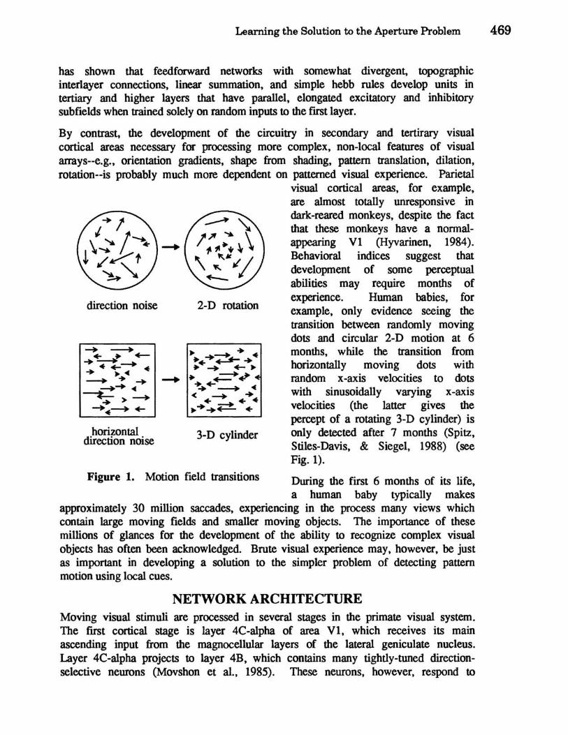
By contrast, the development of the circuitry in secondary and tertirary visual cortical areas necessary for processing more complex, non-local features of visual arrays--e.g., orientation gradients, shape from shading, pattern translation, dilation, rotation--is probably much more dependent on patterned visual experience. Parietal

direction noise

horizontal direction noise

2-D rotation

3-D cylinder

visual cortical areas, for example, are almost totally unresponsive in dark-reared monkeys, despite the fact that these monkeys have a normal­appearing VI (Hyvarinen, 1984). Behavioral indices suggest that development of some perceptual abilities may require months of experience. Human babies, for example, only evidence seeing the transition between randomly moving dots and circular 2-D motion at 6 months, while the transition from horizontally moving dots with random x -axis velocities to dots with sinusoidally varying X-axIS velocities (the latter gives the percept of a rotating 3-D cylinder) is only detected after 7 months (Spitz, Stiles-Davis, & Siegel, 1988) (see Fig. 1).

Figure 1. Motion field transitions During the first 6 months of its life, a human baby typically makes

approximately 30 million saccades, experiencing in the process many views which contain large moving fields and smaller moving objects. The importance of these millions of glances for the development of the ability to recognize complex visual objects has often been acknowledged. Brute visual experience may. however. be just as important in developing a solution to the simpler problem of detecting pattern motion using local cues.

NETWORK ARCHITECTURE Moving visual stimuli are processed in several stages in the primate visual system. The first cortical stage is layer 4C-alpha of area VI, which receives its main ascending input from the magnocellular layers of the lateral geniculate nucleus. Layer 4C-alpha projects to layer 4B, which contains many tightly-tuned direction­selective neurons (Movshon et aI., 1985). These neurons, however, respond to

470 Sereno

moving contours as if these contours were moving perpendicular their local orientation--Le .• they fire in proportion to the difference between the orthogonal component of motion and their best direction (for a bar). An orientation series run for a layer 4B nemon using a plaid (2 orthogonal moving gratings) thus results in two peaks in the direction tuning curve. displaced 45 degrees to either side of the peak for a single grating (Movshon et al.. 1985). The aperture problem for pattern motion (see e.g .• Horn & Schunck. 1981) thus exists for cells in area VI of the adult (and presumably infant) primate.

Layer 4B neurons project topographically via direct and indirect pathways to area MT. a small exttastriate area specialized for processing moving stimuli. A subset

Input Layer

(=Vl, layer 4B)

Second Layer

(=MT)

I \ i

\ / \ /

Figure 2. Network Architecture

of neurons in MT show a single peak in their direction tuning curves for a plaid that is lined up with the peak for a single grating--Le., they fire in proportion to the difference between the true pattern direction and their best direction (for a bar). These neurons therefore solve the aperture problem presented to them by the local translational motion detectors in layer 4B of VI. The excitatory receptive fields of all MT neurons are much larger than those in VI as a result of divergence in the VI­MT projection as well as the smaller areal extent of MT compared to VI.

M.E. Sereno (1987) showed using a supervised learning rule that a linear t two layer network can satisfactorily solve the aperture problem characterized above. The present task was to see if unsupervised learning might suffice. A simple caraicature of the Vl-to-MT projection was constructed. At each x-y location in the first layer of the network. there are a set of units tuned to a range of local directions and speeds. The input layer thus has four dimensions. The sample network illustrated above (Fig. 2) has 5 different directions and 3 speeds at each x-y location. Input units are granted tuning curves resembling those found for neurons in layer 4B of

Learning the Solution to the Aperture Problem 471

~:~ o X 2X

velocity component orthogonal to contour

=pl L>\t)(\ o I I

o 0.5 speed component

orthogonal to contour

Figure 3. Excitatory Tuning Curves (1st layer)

1

area VI. The tuning curves are linear. with half-height overlap for both direction and speed (see Fig. 3--for 12 directions and 4 speeds). and direction and speed tuning interact linearly. Inhibition is either tuned or untuned (see Fig. 4). and scaled to balance excitation. Since direction tuning wraps around. there is a trough in the tuned inhibition condition. Speed tuning does not wrap around. The relative effect of direction and speed tuning in the output of ftrst layer units is set by a parameter.

As with Linsker. the probability that a unit in the fust layer will connect with a unit in the second layer falls off as a gaussian centered on the retinotopically

resp

o

resp

o

untuned 1\ tuned

~[""""""'" ~""'""""". \,. u: ........................ .

o X velocity component

orthogonal to contour

............... ........................

o 0.5 speed component orthogonal to contour (no wrap-around)

2X

1

Figure 4. Tuned vs. Untuned Inhibition

472 Sereno

equivalent point in the second layer (see Fig. 2). New random numbers are drawn to generate the divergent gaussian projection pattern for each first layer unit (Le., all of the units at a single x-y location have different. overlapping projection patterns). There are no local connections within a layer.

The network update rule is similar to that of Linsker except that there is no term like a decay of synaptic weights (k1) and no offset parameter for the correlations (k,J. Also, all of the units in each layer are modeled explicitly. The activation, Yj'

for each unit is a linear weighted sum of its Ui inputs, scaled by a, and clipped to a

maximum or minimum value:

{a I. u· w·· I I)

y. = )

Ymax.min

Weights are also clipped to maximum and minimum values. The change in each weight. .1wij, is a simple fraction, a, of the product of the pre- and post-synaptic values:

.1w·· = au·y· I) I )

RESULTS The network is tr:ained with a set of fullfield texture movements. Each stimulus consists of a set of randomly oriented contours--one at each x-y point--all moving in the same, randomly chosen pattern direction. A typical stimulus is drawn in figure 5 as the set of component motions visible to neurons in VI (i.e .• direction components perpendicular to the local contour); the local speed component varies as the cosine of the angle between the pattern direction and the perpendicular to the local contour. The single component motion at each point is run through the first layer tuning curves. The response of the input layer to such a pattern is shown in Figure 6. Each rectangular box represents a single x-y location, containing 48 units

--./'

--........

~

'-

........ v t- v , .... ....... " ~ ~ I' " ~

" ~ t- ...... .-. '. ? '" .-. -+ ...... ? --I' /' -.. , ~ ...... "- "- ....... .-. ....... .. '-

--+ ./' I' ~ -- ~ --+ " 1 -.. "- "- I'

'- , ./' , A "- "- ...... II' " -+ /' "-v 1 ., .-. " ~ "- A .- /' ~ ./' -+

Figure 5. Local Compqnent Motions from a Training Stimulus (pattern direction is toward right)

.. -.

f

., , /'

Learning the Solution to the Aperture Problem 473

p. . . . • • • . [J • • • o • • • • • ••• 0 • ••

• • • . . . • • • [J D· •• . . . . · Q. • •••• c •••••• ·0····· ·00··

. . . . . . . • • • • • • • 0 • • • •

· .. ·0·

· . 00 .. • • • • • a a • • • · . . . .

• 0 a • · . . . · ... 00· ..

-0-.· -ac- .... ·Da .•••• aa •••••• -0- •••••• 0 ••••••••••••• 0 .••••••• aa ••••. ••••• · . . . . • • • • • • • • • • • • • 0 • • • • •

• • • D • • • • • • • • • • a a • • • • • • • • J • • • • • • .•. 00· .• • • •• C ••• · 00 · · · · • ., • • • • • • • • • • C • • • • •

~ • • •••••••• 0 ••

0-. • • • •• • • •• • • • c·· • • • • 0 • • • • • • • • • • • • • • 0 • • • • • • • • • • • • • • 0 • • • • • • • • • •

• ••. 00 . · ... aD· . . . . . . . ·0· . .

· ald· • 0 . · · •

• • • • • • • • • C • • • • • • • • • • • D a • • • • • . 0 a . . .•• • . a 0 •••••

Figure 6. Output of Portion of First Layer to a Training Slimulus (untuned inhibition)

tuned to different combinations of direction and speed (12 directions run horizontally and 4 speeds run vertically). Open and filled squares indicate positive

and negative outputs. Inhibition is untuned here. The hebb sensitivity, a, was set so that 1,000 such patterns could be presented before most weights saturated at maximum values. Weights intially had small random values drawn from a flat distribution centered around zero. The scale parameter for the weighted sum, a, was set low enough to prevent second layer units from saturating all the time. In Figure 6, direction tuning is 2.5 times as important as speed tuning in detennining the output of a unit

Selectivity of second layer units for pattern direction was examined both before and after training using four stimulus conditions: 1) grating--contours perpendicular to pattern direction, 2) random grating--contours randomly oriented with respect to pattern direction (same as the training condition), 3) plaid--contours oriented 45 or 67 degrees from perpendicular to pattern direction, 4) random plaid--contours randomly oriented, but avoiding angles nearly perpendicular to pattern direction. The pre-training direction tuning curves for the grating conditions usually showed some weak direction selectivity. Pre-training direction tuning curves for the plaid conditions, however, were often twin-peaked, exhibiting pattern component responses displaced to either side of the grating peak. Mter training, by contrast, the direction tuning peaks in all test conditions were single and sharp, and the plaid condition peaks were usually aligned with the grating peaks.

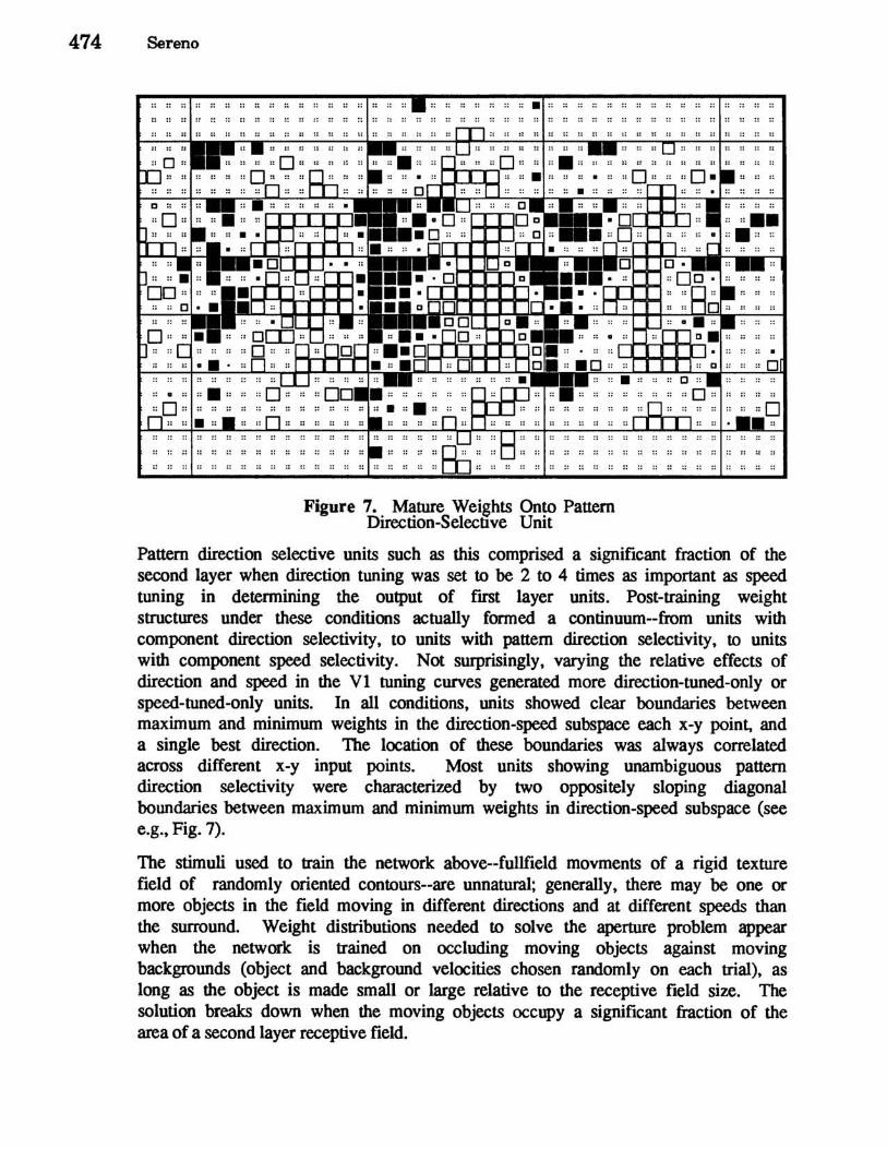
An example of the weights onto a mature pattern direction selective unit is shown in Figure 7. As before, each rectangular box contains 48 units representing one point in x-y space of the input layer (the tails of the 2-D gaussian are cropped in this illustration), except that the black and white boxes now represent negative and positive weights onto a single second layer unit. Within each box, 12 directions run horizontally and 4 speeds run vertically. The peaks in the direction tuning curves for gratings and 135 degree plaids for this unit were sharp and aligned.

474 Sereno

.. :: :: :: "

...... .. .. .. .. .. ...... .. .. .. :: . :: ::

Figure 7. Mature Weights Onto Pattern Direction-Selective Unit

Pattern direction selective units such as this comprised a significant fraction of the second layer when direction tuning was set to be 2 to 4 times as important as speed tuning in determining the output of fU'St layer units. Post-training weight structures under these conditions actually formed a continuum--from units with component direction selectivity, to units with pattern direction selectivity, to units with component speed selectivity. Not surprisingly, varying the relative effects of direction and speed in the VI tuning curves generated more direction-tuned-only or speed-tuned-only units. In all conditions, units showed clear boundaries between maximum and minimum weights in the direction-speed subspace each x-y point, and a single best direction. The location of these boundaries was always correlated across different x-y input points. Most units showing unambiguous pattern direction selectivity were characterized by two oppositely sloping diagonal boundaries between maximum and minimum weights in direction-speed subspace (see e.g., Fig. 7).

The stimuli used to train the network above--fullfield movrnents of a rigid texture field of randomly oriented contours--are unnatural; generally, there may be one or more objects in the field moving in different directions and at different speeds than the surround. Weight distributions needed to solve the aperture problem appear when the network. is trained on occluding moving objects against moving backgrounds (object and background velocities chosen randomly on each trial), as long as the object is made small or large relative to the receptive field size. The solution breaks down when the moving objects occupy a significant fraction of the area of a second layer receptive field.

Learning the Solution to the Aperture Problem 475

For comparison, the network was also trained using two different kinds of noise stimuli. In the fIrst condition (unit noise), each new stimulus consisted of random input values on each input unit With other network parameters held the same, the typical mature weight pattern onto a second layer unit showed an intimate intermixture of maximum and minimum weights in the direction-speed subspace at each x-y location. In the second condition (direction noise), each new stimulus consisted of a random direction at each x-y location. The mature weight patterns now showed continuous regions of all-maximum or all-minimum weights in the speed-direction supspace at each x-y point. In contrast to the situation with fullfieid texture movement stimuli, however, the best directions at each of the x-y points providing input to a given unit were uncorrelated. In addition, multiple best directions at a single x-y point sometimes appeared.

DISCUSSION This simple model suggests that it may be possible to learn the solution to the aperture problem for pattern motion using only biologically realistic unsupervised learning and minimally structured motion fields. Using a similar network architecture, M.E. Sereno had previously shown that supervised learning on the problem of detecting pattern motion direction from local cues leads to the emergence of chevron shaped weight structures in direction-speed space (M.E. Sereno, 1986). The weight structures generated here are similar except that the inside or outside of the chevron is filled in, and upside-down chevrons are more common. This results in decreased selectivity to pattern speed in the second layer.

The model needs to be extended to more complex motion correlations in the input-­e.g., rotation, dilation, shear, multiple objects, flexible objects. MT in primates does not respond selectively to rotation or dilation, while its target area MST does. Thus, biological estimates of rotation and dilation are made in two stages--rotation and dilation are not detected locally, but instead constructed from estimates of local translation. Higher layers in the present model may be able to learn interesting 'second-order' things about rotation, dilation, segmentation, and transparency.

The real primate visual system, of course, has a great many more parts than this model. There are a large number of interconnected cortical visual areas--perbaps as many as 25. A substantial portion of the 600 possible between-area connections may be present (for review, see M.I. Sereno, 1988). There are at least 6 map-like visual structures, and several more non-retinotopic visual structures in the thalamus (beyond the dLGN) that interconnect with the cortical visual areas. Each visual cortical area then has its own set of layers and intedayer connections. The most unbiological aspect of this model is the lack of time and the crude methods of gain control (clipped synaptic weights and input/output functions). Future models should employ within-area connections and time-dependent hebb rules.

Making a biologically realistic model of intermediate and higher level visual processing is difficult since it ostensibly requires making a biologically realistic model of earlier, yet often not less complex stations in the system--e.g., the retina,

476 Sereno

dLGN, and layer 4C of primary visual cortex in the present case. One way to avoid having to model all of the stations up to the one of interest is to use physiological data about how the earlier stations respond to various stimuli, as was done in the present model. This shortcut is applicable to many other problems in modeling the visual system. In order for this to be most effective, physiologists and modelers need to cooperate in generating useful libraries of response profiles to arbitrary stimuli. Many stimulus parameters interact, often nonlinearly, to produce the final output of a cell. In the case of simple moving stimuli in VI and MT, we minimally need to know the interaction between stimulus size, stimulus speed, stimulus direction, surround speed, surround direction, and x-y starting point of the movement relative to the classical excitatory receptive field. Collecting this many response combinations from single cells requires faster serial presentation of stimuli is customary in visual physiology experiments. There is no obvious reason, however, why the rate of stimulus presentation need be any less than the rate at which the visual system nonnally operates--namely, 3-5 new views per second.

Also, we need to get a better understanding of the 'stimulus set'. The very large set of stimuli on which the real visual system is trained (millions of views) is still very poorly characterized. It would be worthwhile and practical, nevertheless, to collect a naturalistic corpus of perhaps 1000 views (several hours of viewing).

Acknowledgements

I thank M.E. Sereno and U. Wehmeier for discussions and comments. Supported by NIH grant F32 EY05887. Networks and displays were constructed on the Rochester Connectionist Simulator.

References

B.K.P. Hom & B.G. Schunck. Determining optical flow. Artiflntell., 17, 185-203 (1981).

J. Hyvarinen. The Parietal Cortex. Springer-Verlag (1984).

R. Linsker. From basic network principles to neural architecture: emergence of orientation-selective cells. Proc. Nat. Acad. Sci. 83,8390-8394 (1986).

J.A. Movshon, E.H. Adelson, M.S. Gizzi & W.T. Newsome. Analysis of moving visual patterns. In Pattern Recognition Mechanisms. Springer-Verlag, pp. 117-151 (1985).

M.E. Sereno. Modeling stages of motion processing in neural networks. Proc. 9th Ann. Con! Cog. Sci. Soc. pp. 405416 (1987).

M.I. Sereno. The visual system. In I.W.v. Seelen, U.M. Leinhos, & G. Shaw (eds.), Organization of Neural Networks. VCH, pp. 176-184 (1988).

R.V. Spitz, J. Stiles-Daves & R.M. Siegel. Infant perception of rotation from rigid structure-from-motion displays. Neurosci. Abstr. 14, 1244 (1988).