Learning to Discover Novel Visual Categories via Deep Transfer Clustering

Kai Han Andrea Vedaldi Andrew Zisserman

Visual Geometry Group, University of Oxford

{khan, vedaldi, az}@robots.ox.ac.uk

Abstract

We consider the problem of discovering novel object cat-

egories in an image collection. While these images are un-

labelled, we also assume prior knowledge of related but

different image classes. We use such prior knowledge to

reduce the ambiguity of clustering, and improve the qual-

ity of the newly discovered classes. Our contributions are

twofold. The first contribution is to extend Deep Embed-

ded Clustering to a transfer learning setting; we also im-

prove the algorithm by introducing a representation bottle-

neck, temporal ensembling, and consistency. The second

contribution is a method to estimate the number of classes

in the unlabelled data. This also transfers knowledge from

the known classes, using them as probes to diagnose dif-

ferent choices for the number of classes in the unlabelled

subset. We thoroughly evaluate our method, substantially

outperforming state-of-the-art techniques in a large num-

ber of benchmarks, including ImageNet, OmniGlot, CIFAR-

100, CIFAR-10, and SVHN.

1. Introduction

With modern supervised learning methods, machines

can recognize thousands of visual categories with high reli-

ability; in fact, machines can outperform individual humans

when performance depends on extensive domain-specific

knowledge as required for example to recognize hundreds

of species of dogs in ImageNet [11]. However, it is also

clear that machines are still far behind human intelligence

in some fundamental ways. A prime example is the fact

that good recognition performance can only be obtained if

computer vision algorithms are manually supervised. Mod-

ern machine learning methods have little to offer in an

open world setting, in which image categories are not de-

fined a-priori, or for which no labelled data is available. In

other words, machines lack an ability to structure data auto-

matically, understanding concepts such as object categories

without external supervision.

In this paper, we study the problem of discovering

and recognizing visual categories automatically. However,

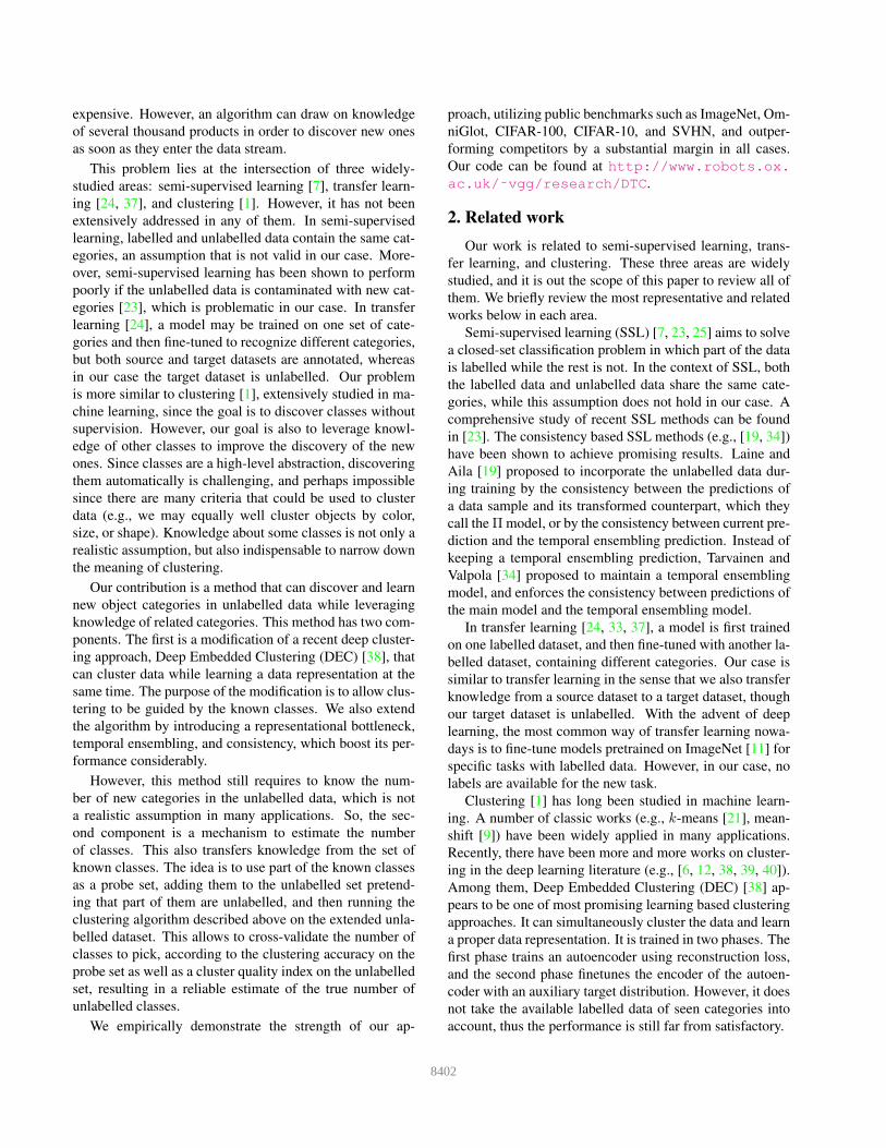
Model

Cat Dog

Labelled training data

Unlabelled data of novel categories Clustering assignment

Transfer

Model

Figure 1. Learning to discover novel visual categories via deep

transfer clustering. We first train a model with labelled images

(e.g., cat and dog). The model is then applied to images of un-

labelled novel categories (e.g., bird and monkey), which transfers

the knowledge learned from the labelled images to the unlabelled

images. With such transferred knowledge, our model can then si-

multaneously learn a feature representation and the clustering as-

signment for the unlabelled images of novel categories.

rather than considering a fully unsupervised setting, we as-

sume that the machine already possesses certain knowledge

about some of the categories in the world. Then, given ad-

ditional images that belong to new categories, the problem

is to tell how many new categories there are and to learn

to recognize them. The aim is to guide this process by

transferring knowledge from the old classes to the new ones

(see fig. 1).

This approach is motivated by the following observation.

Unlike existing machine learning models, a child can eas-

ily tell an unseen animal category (e.g., bird) after learning

a few other (seen) animal categories (e.g., cat, dog); and

an adult wandering around a zoo or wildlife park can ef-

fortlessly discover new categories of animals (e.g., okapi)

based on the many categories previously learnt. In fact,

while we can manually annotate some categories in the

world, we cannot annotate them all, even in relatively re-

stricted settings. For example, consider the problem of rec-

ognizing products in supermarkets for the purpose of mar-

ket research: hundreds of new products are introduced every

week and providing manual annotations for all is hopelessly

18401

expensive. However, an algorithm can draw on knowledge

of several thousand products in order to discover new ones

as soon as they enter the data stream.

This problem lies at the intersection of three widely-

studied areas: semi-supervised learning [7], transfer learn-

ing [24, 37], and clustering [1]. However, it has not been

extensively addressed in any of them. In semi-supervised

learning, labelled and unlabelled data contain the same cat-

egories, an assumption that is not valid in our case. More-

over, semi-supervised learning has been shown to perform

poorly if the unlabelled data is contaminated with new cat-

egories [23], which is problematic in our case. In transfer

learning [24], a model may be trained on one set of cate-

gories and then fine-tuned to recognize different categories,

but both source and target datasets are annotated, whereas

in our case the target dataset is unlabelled. Our problem

is more similar to clustering [1], extensively studied in ma-

chine learning, since the goal is to discover classes without

supervision. However, our goal is also to leverage knowl-

edge of other classes to improve the discovery of the new

ones. Since classes are a high-level abstraction, discovering

them automatically is challenging, and perhaps impossible

since there are many criteria that could be used to cluster

data (e.g., we may equally well cluster objects by color,

size, or shape). Knowledge about some classes is not only a

realistic assumption, but also indispensable to narrow down

the meaning of clustering.

Our contribution is a method that can discover and learn

new object categories in unlabelled data while leveraging

knowledge of related categories. This method has two com-

ponents. The first is a modification of a recent deep cluster-

ing approach, Deep Embedded Clustering (DEC) [38], that

can cluster data while learning a data representation at the

same time. The purpose of the modification is to allow clus-

tering to be guided by the known classes. We also extend

the algorithm by introducing a representational bottleneck,

temporal ensembling, and consistency, which boost its per-

formance considerably.

However, this method still requires to know the num-

ber of new categories in the unlabelled data, which is not

a realistic assumption in many applications. So, the sec-

ond component is a mechanism to estimate the number

of classes. This also transfers knowledge from the set of

known classes. The idea is to use part of the known classes

as a probe set, adding them to the unlabelled set pretend-

ing that part of them are unlabelled, and then running the

clustering algorithm described above on the extended unla-

belled dataset. This allows to cross-validate the number of

classes to pick, according to the clustering accuracy on the

probe set as well as a cluster quality index on the unlabelled

set, resulting in a reliable estimate of the true number of

unlabelled classes.

We empirically demonstrate the strength of our ap-

proach, utilizing public benchmarks such as ImageNet, Om-

niGlot, CIFAR-100, CIFAR-10, and SVHN, and outper-

forming competitors by a substantial margin in all cases.

Our code can be found at http://www.robots.ox.

ac.uk/˜vgg/research/DTC.

2. Related work

Our work is related to semi-supervised learning, trans-

fer learning, and clustering. These three areas are widely

studied, and it is out the scope of this paper to review all of

them. We briefly review the most representative and related

works below in each area.

Semi-supervised learning (SSL) [7, 23, 25] aims to solve

a closed-set classification problem in which part of the data

is labelled while the rest is not. In the context of SSL, both

the labelled data and unlabelled data share the same cate-

gories, while this assumption does not hold in our case. A

comprehensive study of recent SSL methods can be found

in [23]. The consistency based SSL methods (e.g., [19, 34])

have been shown to achieve promising results. Laine and

Aila [19] proposed to incorporate the unlabelled data dur-

ing training by the consistency between the predictions of

a data sample and its transformed counterpart, which they

call the Π model, or by the consistency between current pre-

diction and the temporal ensembling prediction. Instead of

keeping a temporal ensembling prediction, Tarvainen and

Valpola [34] proposed to maintain a temporal ensembling

model, and enforces the consistency between predictions of

the main model and the temporal ensembling model.

In transfer learning [24, 33, 37], a model is first trained

on one labelled dataset, and then fine-tuned with another la-

belled dataset, containing different categories. Our case is

similar to transfer learning in the sense that we also transfer

knowledge from a source dataset to a target dataset, though

our target dataset is unlabelled. With the advent of deep

learning, the most common way of transfer learning nowa-

days is to fine-tune models pretrained on ImageNet [11] for

specific tasks with labelled data. However, in our case, no

labels are available for the new task.

Clustering [1] has long been studied in machine learn-

ing. A number of classic works (e.g., k-means [21], mean-

shift [9]) have been widely applied in many applications.

Recently, there have been more and more works on cluster-

ing in the deep learning literature (e.g., [6, 12, 38, 39, 40]).

Among them, Deep Embedded Clustering (DEC) [38] ap-

pears to be one of most promising learning based clustering

approaches. It can simultaneously cluster the data and learn

a proper data representation. It is trained in two phases. The

first phase trains an autoencoder using reconstruction loss,

and the second phase finetunes the encoder of the autoen-

coder with an auxiliary target distribution. However, it does

not take the available labelled data of seen categories into

account, thus the performance is still far from satisfactory.

8402

Our work is also related to metric learning [29, 30, 31]

and domain adaptation [36]. Actually, we build on metric

learning, as the latter is used for initialization. However,

most metric learning methods are unable to exploit unla-

belled data, while our work can automatically adjust the

embeddings space on unlabelled data. More importantly,

our task requires producing a partition of the data (a dis-

crete decision), whereas metric learning only produces a

continuous data embedding, and converting the latter to dis-

crete classes is often not trivial. Domain adaptation aims

to resolve the domain discrepancy between source and tar-

get datasets (e.g., digital SLR camera images vs web cam-

era images), while generally assuming a shared class space.

Thus, the source and target data are on different manifolds.

In our case, the unlabelled data belongs to novel categories

without any labels, and the unlabelled data are on the same

manifold with the labelled data, which is a more practical

but more challenging scenario.

To our knowledge, the most related works to ours

are [15] and [16], in terms of considering novel visual cat-

egory discovery as a deep transfer clustering task. In [15],

Hsu et al. introduced a Constrained Clustering Network

(CCN) which is trained in two stages. In the first stage,

a binary classification model is trained on labelled data to

measure pair-wise similarity of images. In the second stage,

a clustering model is trained on unlabelled data by using

the output of the binary classification model as supervision.

The network is trained with a Kullback-Leibler divergence

based contrastive loss (KCL). In [16], the CCN is improved

by replacing KCL with a new loss called Meta Classifica-

tion Likelihood (MCL). In addition, Huang et al. [17] re-

cently introduced Centroid Networks for few-shot cluster-

ing, which cluster K×M unlabeled images into K clusters

with M images each after training on labeled data.

3. Deep transfer clustering

We propose a method for data clustering: given as input

an unlabelled dataset Du = {xui , i = 1, . . . ,M}, usually of

images, the goal is to produce as output class assignments

yui ∈ {1, . . . ,K}, where the number of different classes Kis unknown. Since there can be multiple equally-valid crite-

ria for clustering data, making a choice depends on the ap-

plication. Thus, we also assume we have a labelled dataset

Dl = {(xli, y

li), i = 1, . . . , N} where class assignments

yli ∈ {1, . . . , L} are known.

The classes in this labelled set differ, in identity and

number, from the classes in the unlabelled set. Hence the

goal is to learn from the labelled data not its specific classes,

but what properties make a good class in general, so that this

knowledge can be used to discover new classes and their

number in the unlabelled data.

We propose a method with two components. The first is

an extension of a deep clustering algorithm that can transfer

knowledge from a known set of classes to a new one (sec-

tion 3.1); the second is a method to reliably estimate the

number of unlabelled classes K (section 3.2).

3.1. Transfer clustering and representation learning

At its core, our method is based on a deep clustering al-

gorithm that clusters the data while simultaneously learning

a good data representation. We extract this representation

by applying a neural network fθ to the data, obtaining em-

bedding vectors z = fθ(x) ∈ Rd. The representation is

initialised using the labelled data, and then fine-tuned using

the unlabelled data. This is done via deep embedded cluster-

ing (DEC) of [38] with three important modifications: the

method is extended to account for labelled data, to include a

tight bottleneck to improve generalization, and to incorpo-

rate temporal ensembling and consistency, which also con-

tribute to its stability and performance. An overview of our

approach is given in algorithm 1.

3.1.1 Joint clustering and representation learning

In this section we summarise DEC [38] as this algorithm

lies at the core of our approach. In DEC, similar to k-means,

clusters are represented by a collection of vectors or proto-

types U = {µk, k = 1, . . . ,K} representing the cluster

“centers”. However, differently from k-means, the goal is

not only to determine the clusters, but also to learn the data

representation fθ.

Naively combining representation learning, which is a

discriminative task, and clustering, which is a generative

one, is challenging. For instance, directly minimizing the

k-means objective function would immediately collapse the

learned representation vectors to the closest cluster centers.

DEC [38] addresses this problem by slowly annealing clus-

ter centers and data representation.

In order to do so, let p(k|i) be the probability of assign-

ing data point i ∈ {1, . . . , N} to cluster k ∈ {1, . . . ,K}.

DEC uses the following parameteterization of this condi-

tional distribution by assuming a Student’s t distribution:

p(k|i) ∝

(

1 +‖zi − µk‖

2

α

)−α+1

2

. (1)

Further assuming that data indices are sampled uniformly

(i.e. p(i) = 1/N ), we can write the joint distribution

p(i, k) = p(k|i)/N .

In order to anneal to a good solution, instead of maxi-

mizing the likelihood of the model p directly, we match the

model to a suitably-shaped distribution q. This is done by

minimizing the KL divergence between joint distributions

q(i, k) = q(k|i)/N and p(i, k) = p(k|i)/N , given by

E(q) = KL(q||p) =1

N

N∑

i=1

K∑

k=1

q(k|i) logq(k|i)

p(k|i). (2)

8403

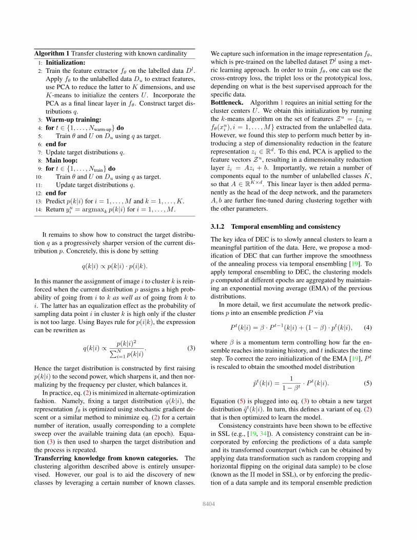
Algorithm 1 Transfer clustering with known cardinality

1: Initialization:

2: Train the feature extractor fθ on the labelled data Dl.

Apply fθ to the unlabelled data Du to extract features,

use PCA to reduce the latter to K dimensions, and use

K-means to initialize the centers U . Incorporate the

PCA as a final linear layer in fθ. Construct target dis-

tributions q.

3: Warm-up training:

4: for t ∈ {1, . . . , Nwarm-up} do

5: Train θ and U on Du using q as target.

6: end for

7: Update target distributions q.

8: Main loop:

9: for t ∈ {1, . . . , Ntrain} do

10: Train θ and U on Du using q as target.

11: Update target distributions q.

12: end for

13: Predict p(k|i) for i = 1, . . . ,M and k = 1, . . . ,K.

14: Return yui = argmaxk p(k|i) for i = 1, . . . ,M .

It remains to show how to construct the target distribu-

tion q as a progressively sharper version of the current dis-

tribution p. Concretely, this is done by setting

q(k|i) ∝ p(k|i) · p(i|k).

In this manner the assignment of image i to cluster k is rein-

forced when the current distribution p assigns a high prob-

ability of going from i to k as well as of going from k to

i. The latter has an equalization effect as the probability of

sampling data point i in cluster k is high only if the cluster

is not too large. Using Bayes rule for p(i|k), the expression

can be rewritten as

q(k|i) ∝p(k|i)2

∑N

i=1 p(k|i). (3)

Hence the target distribution is constructed by first raising

p(k|i) to the second power, which sharpens it, and then nor-

malizing by the frequency per cluster, which balances it.

In practice, eq. (2) is minimized in alternate-optimization

fashion. Namely, fixing a target distribution q(k|i), the

representation fθ is optimized using stochastic gradient de-

scent or a similar method to minimize eq. (2) for a certain

number of iteration, usually corresponding to a complete

sweep over the available training data (an epoch). Equa-

tion (3) is then used to sharpen the target distribution and

the process is repeated.

Transferring knowledge from known categories. The

clustering algorithm described above is entirely unsuper-

vised. However, our goal is to aid the discovery of new

classes by leveraging a certain number of known classes.

We capture such information in the image representation fθ,

which is pre-trained on the labelled dataset Dl using a met-

ric learning approach. In order to train fθ, one can use the

cross-entropy loss, the triplet loss or the prototypical loss,

depending on what is the best supervised approach for the

specific data.

Bottleneck. Algorithm 1 requires an initial setting for the

cluster centers U . We obtain this initialization by running

the k-means algorithm on the set of features Zu = {zi =fθ(x

ui ), i = 1, . . . ,M} extracted from the unlabelled data.

However, we found this step to perform much better by in-

troducing a step of dimensionality reduction in the feature

representation zi ∈ Rd. To this end, PCA is applied to the

feature vectors Zu, resulting in a dimensionality reduction

layer zi = Azi + b. Importantly, we retain a number of

components equal to the number of unlabelled classes K,

so that A ∈ RK×d. This linear layer is then added perma-

nently as the head of the deep network, and the parameters

A, b are further fine-tuned during clustering together with

the other parameters.

3.1.2 Temporal ensembling and consistency

The key idea of DEC is to slowly anneal clusters to learn a

meaningful partition of the data. Here, we propose a mod-

ification of DEC that can further improve the smoothness

of the annealing process via temporal ensembling [19]. To

apply temporal ensembling to DEC, the clustering models

p computed at different epochs are aggregated by maintain-

ing an exponential moving average (EMA) of the previous

distributions.

In more detail, we first accumulate the network predic-

tions p into an ensemble prediction P via

P t(k|i) = β · P t−1(k|i) + (1− β) · pt(k|i), (4)

where β is a momentum term controlling how far the en-

semble reaches into training history, and t indicates the time

step. To correct the zero initialization of the EMA [19], P t

is rescaled to obtain the smoothed model distribution

pt(k|i) =1

1− βt· P t(k|i). (5)

Equation (5) is plugged into eq. (3) to obtain a new target

distribution qt(k|i). In turn, this defines a variant of eq. (2)

that is then optimized to learn the model.

Consistency constraints have been shown to be effective

in SSL (e.g., [19, 34]). A consistency constraint can be in-

corporated by enforcing the predictions of a data sample

and its transformed counterpart (which can be obtained by

applying data transformation such as random cropping and

horizontal flipping on the original data sample) to be close

(known as the Π model in SSL), or by enforcing the predic-

tion of a data sample and its temporal ensemble prediction

8404

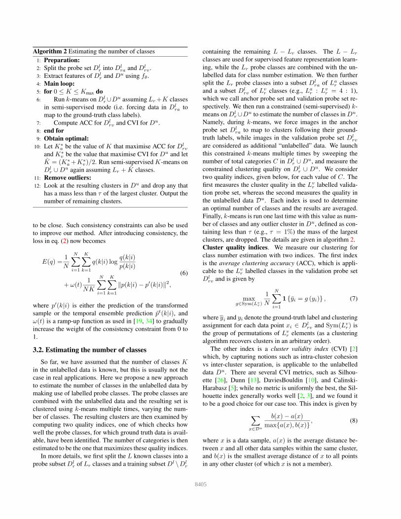
Algorithm 2 Estimating the number of classes

1: Preparation:

2: Split the probe set Dlr into Dl

ra and Dlrv .

3: Extract features of Dlr and Du using fθ.

4: Main loop:

5: for 0 ≤ K ≤ Kmax do

6: Run k-means on Dlr∪Du assuming Lr+K classes

in semi-supervised mode (i.e. forcing data in Dlra to

map to the ground-truth class labels).

7: Compute ACC for Dlrv and CVI for Du.

8: end for

9: Obtain optimal:

10: Let K∗a be the value of K that maximise ACC for Dl

rv

and K∗v be the value that maximise CVI for Du and let

K = (K∗a +K∗

v )/2. Run semi-supervised K-means on

Dlr ∪Du again assuming Lr + K classes.

11: Remove outliers:

12: Look at the resulting clusters in Du and drop any that

has a mass less than τ of the largest cluster. Output the

number of remaining clusters.

to be close. Such consistency constraints can also be used

to improve our method. After introducing consistency, the

loss in eq. (2) now becomes

E(q) =1

N

N∑

i=1

K∑

k=1

q(k|i) logq(k|i)

p(k|i)

+ ω(t)1

NK

N∑

i=1

K∑

k=1

‖p(k|i)− p′(k|i)‖2,

(6)

where p′(k|i) is either the prediction of the transformed

sample or the temporal ensemble prediction pt(k|i), and

ω(t) is a ramp-up function as used in [19, 34] to gradually

increase the weight of the consistency constraint from 0 to

1.

3.2. Estimating the number of classes

So far, we have assumed that the number of classes Kin the unlabelled data is known, but this is usually not the

case in real applications. Here we propose a new approach

to estimate the number of classes in the unlabelled data by

making use of labelled probe classes. The probe classes are

combined with the unlabelled data and the resulting set is

clustered using k-means multiple times, varying the num-

ber of classes. The resulting clusters are then examined by

computing two quality indices, one of which checks how

well the probe classes, for which ground truth data is avail-

able, have been identified. The number of categories is then

estimated to be the one that maximizes these quality indices.

In more details, we first split the L known classes into a

probe subset Dlr of Lr classes and a training subset Dl \Dl

r

containing the remaining L − Lr classes. The L − Lr

classes are used for supervised feature representation learn-

ing, while the Lr probe classes are combined with the un-

labelled data for class number estimation. We then further

split the Lr probe classes into a subset Dlra of La

r classes

and a subset Dlrv of Lv

r classes (e.g., Lar : Lv

r = 4 : 1),

which we call anchor probe set and validation probe set re-

spectively. We then run a constrained (semi-supervised) k-

means on Dlr∪Du to estimate the number of classes in Du.

Namely, during k-means, we force images in the anchor

probe set Dlra to map to clusters following their ground-

truth labels, while images in the validation probe set Dlrv

are considered as additional “unlabelled” data. We launch

this constrained k-means multiple times by sweeping the

number of total categories C in Dlr ∪Du, and measure the

constrained clustering quality on Dlr ∪ Du. We consider

two quality indices, given below, for each value of C. The

first measures the cluster quality in the Lvr labelled valida-

tion probe set, whereas the second measures the quality in

the unlabelled data Du. Each index is used to determine

an optimal number of classes and the results are averaged.

Finally, k-means is run one last time with this value as num-

ber of classes and any outlier cluster in Du, defined as con-

taining less than τ (e.g., τ = 1%) the mass of the largest

clusters, are dropped. The details are given in algorithm 2.

Cluster quality indices. We measure our clustering for

class number estimation with two indices. The first index

is the average clustering accuracy (ACC), which is appli-

cable to the Lvr labelled classes in the validation probe set

Dlrv and is given by

maxg∈Sym(Lv

r)

1

N

N∑

i=1

1 {yi = g (yi)} , (7)

where yi and yi denote the ground-truth label and clustering

assignment for each data point xi ∈ Dlrv and Sym(Lv

r) is

the group of permutations of Lvr elements (as a clustering

algorithm recovers clusters in an arbitrary order).

The other index is a cluster validity index (CVI) [2]

which, by capturing notions such as intra-cluster cohesion

vs inter-cluster separation, is applicable to the unlabelled

data Du. There are several CVI metrics, such as Silhou-

ette [26], Dunn [13], DaviesBouldin [10], and Calinski-

Harabasz [5]; while no metric is uniformly the best, the Sil-

houette index generally works well [2, 3], and we found it

to be a good choice for our case too. This index is given by

∑

x∈Du

b(x)− a(x)

max{a(x), b(x)}, (8)

where x is a data sample, a(x) is the average distance be-

tween x and all other data samples within the same cluster,

and b(x) is the smallest average distance of x to all points

in any other cluster (of which x is not a member).

8405

4. Experimental results

We assess two scenarios over multiple benchmarks: first,

where the number of new classes is known for OmniGlot,

ImageNet, CIFAR-10, CIFAR-100 and SVHN; and second,

where the number of new classes is unknown for OmniGlot,

ImageNet and CIFAR-100. For the unknown scenario we

separate a probe set from the labelled classes.

4.1. Data and experimental details

OmniGlot [20]. This dataset contains 1,623 handwritten

characters from 50 different alphabets. It is divided into a

30-alphabet (964 characters) subset called background set

and a 20-alphabet (659 characters) subset called evaluation

set. Each character is considered as one category and has

20 example images. We use the background and evaluation

sets as labelled and unlabelled data, respectively. To ex-

periment with an unknown number of classes, we randomly

hold out 5 alphabets from the background set (169 charac-

ters in total) to use as probes for algorithm 2, leaving the

remaining 795 characters to learn the feature extractor.

ImageNet [11]. ImageNet contains 1,000 classes and about

1,000 example images per class. We follow [35] and split

the data into two subsets containing 882 and 118 classes re-

spectively. Following [15, 16], we consider the 882-class

subset as labelled data, and use three randomly sampled 30-

class subsets from the remaining 118-class subset as unla-

belled data. To experiment with an unknown number of

classes, we randomly hold out 82 classes from the 882-

class subset as probes, leaving the remaining 800 classes

for training the feature extractor.

CIFAR-10/CIFAR-100 [18]. CIFAR-10 contains 50,000

training images and 10,000 test images from 10 classes.

Each image has a size of 32× 32. We split the training im-

ages into labelled and unlabelled subsets. In particular, we

consider the images of the first 5 categories (i.e., airplane,

automobile, bird, cat, deer) as the labelled set, while the re-

maining 5 categories (i.e., dog, frog, horse, ship, truck) as

the unlabelled set. CIFAR-100 is similar to CIFAR-10, ex-

cept it has 10 times less images per class. We consider the

first 80 classes as labelled data, and the last 10 classes as

unlabelled data, leaving 10 classes as probe set for category

number estimation on unlabelled data.

SVHN [22]. SVHN contains 73,257 images of digits for

training and 26,032 images for testing. We split the 73,257

training digits into labelled and unlabelled subsets. Namely,

we consider the images of digits 0-4 as the labelled set, and

the images of 5-9 as the unlabelled set. The labelled set

contains 45,349 images, while the unlabelled set contains

27,908 images.

Evaluation metrics. We adopt the conventionally used

clustering accuracy (ACC) and normalized mutual informa-

tion (NMI) [32] to evaluate the clustering performance of

our approach. Both metrics are valued in the range of [0, 1]

and higher values mean better performance. We measure

error in the estimation of the number of novel categories as

|Kgt −Kest|, where Kgt and Kest denote the ground-truth

and estimated number of categories, respectively.

Network architectures. For a fair comparison, we fol-

low [15, 16] and use a 6-layer VGG like architecture [27]

for OmniGlot and CIFAR-100, and a ResNet18 [14] for Im-

ageNet and all other datasets.

Training configurations. OmniGlot is widely used in the

context of few-shot learning due to the very large number

of categories it contains and the small number of example

images per category. Hence, in order to train the feature

extractor on the background set of OmniGlot we use the

prototypical loss [28], one of the best methods for few-shot

learning. We train the feature extractor with a batch size of

200, forming batches by randomly sampling 20 categories

and including 10 images per category. For each category,

5 images are used as supporting data to calculate the proto-

types while the remaining 5 images are used as query sam-

ples. We use Adam optimizer with a learning rate of 0.001

for 200 epochs. We then finetune fθ and train the bottleneck

and the cluster centers U for each alphabet in the evaluation

set. For warm-up (in algorithm 1), the Adam optimizer is

used with a learning rate of 0.001, and trained for 10 epochs

without updating the target distribution. Afterwards, train-

ing continues for another 90 epochs updating the target dis-

tribution per epoch. For ImageNet and other datasets, which

are widely used in supervised image classification tasks, we

pre-train the feature extractor using the cross-entropy loss

on the labelled subsets. Following common practice, we

then remove the last layer of the classification network and

use the the rest of the model as our feature extractor.

In our experiment on ImageNet, we take the pretrained

ImageNet882 classification network of [16] as our initial

feature extractor. For the case when the number of novel

categories is unknown, we train a ImageNet800 classifica-

tion network as our initial feature extractor. We use SGD

with an initial learning rate of 0.1, which is divided by 10

every 30 epochs, for 90 epochs. For warm-up, the feature

extractor, together with the bottleneck and cluster centers,

are trained for 10 epochs by SGD with a learning rate of 0.1;

then, we train for further 60 epochs updating the target dis-

tribution per epoch. Experiments on other datasets follow a

similar configuration. Our results on all datasets are aver-

aged over 10 runs, except ImageNet, which is averaged over

3 runs using different unlabelled subsets following [15, 16].

4.2. Learning with a known number of categories

In table 1 we compare variants of our Deep Transfer

Clustering (DTC) approach with the temporal ensembling

and consistency constraints as introduced in section 3.1.2,

namely, DTC-Baseline (our model trained using DEC loss),

DTC-Π (our model trained using DEC loss with consis-

8406

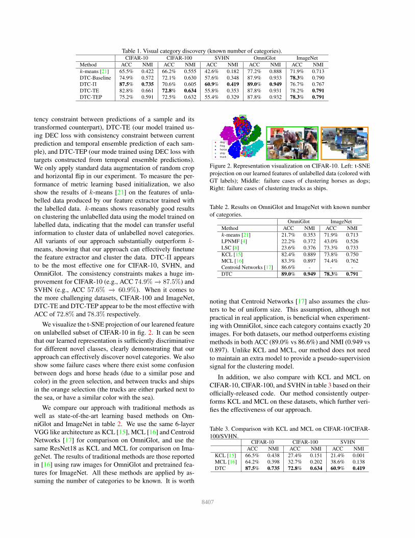
Table 1. Visual category discovery (known number of categories).CIFAR-10 CIFAR-100 SVHN OmniGlot ImageNet

Method ACC NMI ACC NMI ACC NMI ACC NMI ACC NMI

k-means [21] 65.5% 0.422 66.2% 0.555 42.6% 0.182 77.2% 0.888 71.9% 0.713

DTC-Baseline 74.9% 0.572 72.1% 0.630 57.6% 0.348 87.9% 0.933 78.3% 0.790

DTC-Π 87.5% 0.735 70.6% 0.605 60.9% 0.419 89.0% 0.949 76.7% 0.767

DTC-TE 82.8% 0.661 72.8% 0.634 55.8% 0.353 87.8% 0.931 78.2% 0.791

DTC-TEP 75.2% 0.591 72.5% 0.632 55.4% 0.329 87.8% 0.932 78.3% 0.791

tency constraint between predictions of a sample and its

transformed counterpart), DTC-TE (our model trained us-

ing DEC loss with consistency constraint between current

prediction and temporal ensemble prediction of each sam-

ple), and DTC-TEP (our mode trained using DEC loss with

targets constructed from temporal ensemble predictions).

We only apply standard data augmentation of random crop

and horizontal flip in our experiment. To measure the per-

formance of metric learning based initialization, we also

show the results of k-means [21] on the features of unla-

belled data produced by our feature extractor trained with

the labelled data. k-means shows reasonably good results

on clustering the unlabelled data using the model trained on

labelled data, indicating that the model can transfer useful

information to cluster data of unlabelled novel categories.

All variants of our approach substantially outperform k-

means, showing that our approach can effectively finetune

the feature extractor and cluster the data. DTC-Π appears

to be the most effective one for CIFAR-10, SVHN, and

OmniGlot. The consistency constraints makes a huge im-

provement for CIFAR-10 (e.g., ACC 74.9% −→ 87.5%) and

SVHN (e.g., ACC 57.6% −→ 60.9%). When it comes to

the more challenging datasets, CIFAR-100 and ImageNet,

DTC-TE and DTC-TEP appear to be the most effective with

ACC of 72.8% and 78.3% respectively.

We visualize the t-SNE projection of our learened feature

on unlabelled subset of CIFAR-10 in fig. 2. It can be seen

that our learned representation is sufficiently discriminative

for different novel classes, clearly demonstrating that our

approach can effectively discover novel categories. We also

show some failure cases where there exist some confusion

between dogs and horse heads (due to a similar pose and

color) in the green selection, and between trucks and ships

in the orange selection (the trucks are either parked next to

the sea, or have a similar color with the sea).

We compare our approach with traditional methods as

well as state-of-the-art learning based methods on Om-

niGlot and ImageNet in table 2. We use the same 6-layer

VGG like architecture as KCL [15], MCL [16] and Centroid

Networks [17] for comparison on OmniGlot, and use the

same ResNet18 as KCL and MCL for comparison on Ima-

geNet. The results of traditional methods are those reported

in [16] using raw images for OmniGlot and pretrained fea-

tures for ImageNet. All these methods are applied by as-

suming the number of categories to be known. It is worth

Figure 2. Representation visualization on CIFAR-10. Left: t-SNE

projection on our learned features of unlabelled data (colored with

GT labels); Middle: failure cases of clustering horses as dogs;

Right: failure cases of clustering trucks as ships.

Table 2. Results on OmniGlot and ImageNet with known number

of categories.OmniGlot ImageNet

Method ACC NMI ACC NMI

k-means [21] 21.7% 0.353 71.9% 0.713

LPNMF [4] 22.2% 0.372 43.0% 0.526

LSC [8] 23.6% 0.376 73.3% 0.733

KCL [15] 82.4% 0.889 73.8% 0.750

MCL [16] 83.3% 0.897 74.4% 0.762

Centroid Networks [17] 86.6% - - -

DTC 89.0% 0.949 78.3% 0.791

noting that Centroid Networks [17] also assumes the clus-

ters to be of uniform size. This assumption, although not

practical in real application, is beneficial when experiment-

ing with OmniGlot, since each category contains exactly 20

images. For both datasets, our method outperforms existing

methods in both ACC (89.0% vs 86.6%) and NMI (0.949 vs

0.897). Unlike KCL and MCL, our method does not need

to maintain an extra model to provide a pseudo-supervision

signal for the clustering model.

In addition, we also compare with KCL and MCL on

CIFAR-10, CIFAR-100, and SVHN in table 3 based on their

officially-released code. Our method consistently outper-

forms KCL and MCL on these datasets, which further veri-

fies the effectiveness of our approach.

Table 3. Comparison with KCL and MCL on CIFAR-10/CIFAR-

100/SVHN.CIFAR-10 CIFAR-100 SVHN

ACC NMI ACC NMI ACC NMI

KCL [15] 66.5% 0.438 27.4% 0.151 21.4% 0.001

MCL [16] 64.2% 0.398 32.7% 0.202 38.6% 0.138

DTC 87.5% 0.735 72.8% 0.634 60.9% 0.419

8407

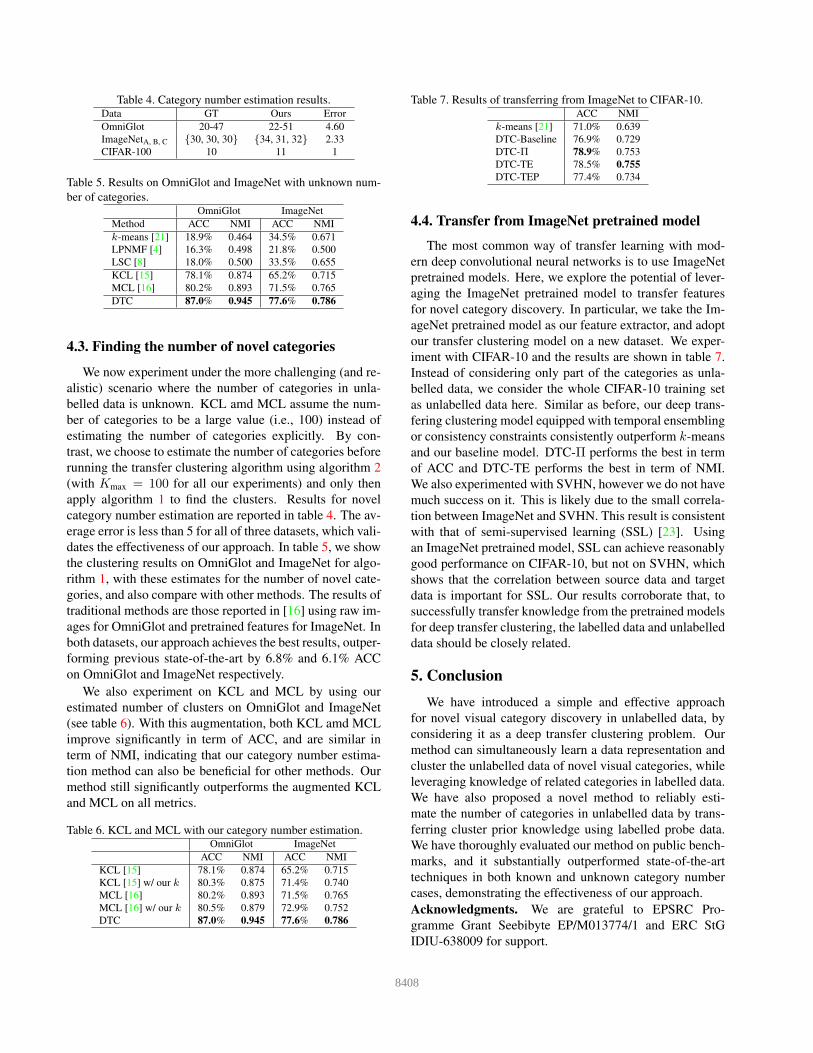
Table 4. Category number estimation results.Data GT Ours Error

OmniGlot 20-47 22-51 4.60

ImageNetA, B, C {30, 30, 30} {34, 31, 32} 2.33

CIFAR-100 10 11 1

Table 5. Results on OmniGlot and ImageNet with unknown num-

ber of categories.OmniGlot ImageNet

Method ACC NMI ACC NMI

k-means [21] 18.9% 0.464 34.5% 0.671

LPNMF [4] 16.3% 0.498 21.8% 0.500

LSC [8] 18.0% 0.500 33.5% 0.655

KCL [15] 78.1% 0.874 65.2% 0.715

MCL [16] 80.2% 0.893 71.5% 0.765

DTC 87.0% 0.945 77.6% 0.786

4.3. Finding the number of novel categories

We now experiment under the more challenging (and re-

alistic) scenario where the number of categories in unla-

belled data is unknown. KCL amd MCL assume the num-

ber of categories to be a large value (i.e., 100) instead of

estimating the number of categories explicitly. By con-

trast, we choose to estimate the number of categories before

running the transfer clustering algorithm using algorithm 2

(with Kmax = 100 for all our experiments) and only then

apply algorithm 1 to find the clusters. Results for novel

category number estimation are reported in table 4. The av-

erage error is less than 5 for all of three datasets, which vali-

dates the effectiveness of our approach. In table 5, we show

the clustering results on OmniGlot and ImageNet for algo-

rithm 1, with these estimates for the number of novel cate-

gories, and also compare with other methods. The results of

traditional methods are those reported in [16] using raw im-

ages for OmniGlot and pretrained features for ImageNet. In

both datasets, our approach achieves the best results, outper-

forming previous state-of-the-art by 6.8% and 6.1% ACC

on OmniGlot and ImageNet respectively.

We also experiment on KCL and MCL by using our

estimated number of clusters on OmniGlot and ImageNet

(see table 6). With this augmentation, both KCL amd MCL

improve significantly in term of ACC, and are similar in

term of NMI, indicating that our category number estima-

tion method can also be beneficial for other methods. Our

method still significantly outperforms the augmented KCL

and MCL on all metrics.

Table 6. KCL and MCL with our category number estimation.OmniGlot ImageNet

ACC NMI ACC NMI

KCL [15] 78.1% 0.874 65.2% 0.715

KCL [15] w/ our k 80.3% 0.875 71.4% 0.740

MCL [16] 80.2% 0.893 71.5% 0.765

MCL [16] w/ our k 80.5% 0.879 72.9% 0.752

DTC 87.0% 0.945 77.6% 0.786

Table 7. Results of transferring from ImageNet to CIFAR-10.ACC NMI

k-means [21] 71.0% 0.639

DTC-Baseline 76.9% 0.729

DTC-Π 78.9% 0.753

DTC-TE 78.5% 0.755

DTC-TEP 77.4% 0.734

4.4. Transfer from ImageNet pretrained model

The most common way of transfer learning with mod-

ern deep convolutional neural networks is to use ImageNet

pretrained models. Here, we explore the potential of lever-

aging the ImageNet pretrained model to transfer features

for novel category discovery. In particular, we take the Im-

ageNet pretrained model as our feature extractor, and adopt

our transfer clustering model on a new dataset. We exper-

iment with CIFAR-10 and the results are shown in table 7.

Instead of considering only part of the categories as unla-

belled data, we consider the whole CIFAR-10 training set

as unlabelled data here. Similar as before, our deep trans-

fering clustering model equipped with temporal ensembling

or consistency constraints consistently outperform k-means

and our baseline model. DTC-Π performs the best in term

of ACC and DTC-TE performs the best in term of NMI.

We also experimented with SVHN, however we do not have

much success on it. This is likely due to the small correla-

tion between ImageNet and SVHN. This result is consistent

with that of semi-supervised learning (SSL) [23]. Using

an ImageNet pretrained model, SSL can achieve reasonably

good performance on CIFAR-10, but not on SVHN, which

shows that the correlation between source data and target

data is important for SSL. Our results corroborate that, to

successfully transfer knowledge from the pretrained models

for deep transfer clustering, the labelled data and unlabelled

data should be closely related.

5. Conclusion

We have introduced a simple and effective approach

for novel visual category discovery in unlabelled data, by

considering it as a deep transfer clustering problem. Our

method can simultaneously learn a data representation and

cluster the unlabelled data of novel visual categories, while

leveraging knowledge of related categories in labelled data.

We have also proposed a novel method to reliably esti-

mate the number of categories in unlabelled data by trans-

ferring cluster prior knowledge using labelled probe data.

We have thoroughly evaluated our method on public bench-

marks, and it substantially outperformed state-of-the-art

techniques in both known and unknown category number

cases, demonstrating the effectiveness of our approach.

Acknowledgments. We are grateful to EPSRC Pro-

gramme Grant Seebibyte EP/M013774/1 and ERC StG

IDIU-638009 for support.

8408

References

[1] Charu C. Aggarwal and Chandan K. Reddy. Data Cluster-

ing: Algorithms and Applications. CRC Press, 2013. 2[2] Olatz Arbelaitz, Ibai Gurrutxaga, Javier Muguerza, JesuS M.

Perez, and InIgo Perona. An extensive comparative study of

cluster validity indices. Pattern Recognition, 2012. 5[3] James C. Bezdek and Nikhil R. Pal. Some new indexes of

cluster validity. IEEE Transactions on Systems, Man, and

Cybernetics, Part B, 1998. 5[4] Deng Cai, Xiaofei He, Xuanhui Wang, Hujun Bao, and Ji-

awei Han. Locality preserving nonnegative matrix factoriza-

tion. In IJCAI, 2009. 7, 8[5] Tadeusz Calinski and JA Harabasz. A dendrite method for

cluster analysis. Communications in Statistics-theory and

Methods, 1974. 5[6] Jianlong Chang, Lingfeng Wang, Gaofeng Meng, Shiming

Xiang, and Chunhong Pan. Deep adaptive image clustering.

In ICCV, 2017. 2[7] Olivier Chapelle, Bernhard Scholkopf, and Alexander Zien.

Semi-Supervised Learning. MIT Press, 2006. 2[8] Xinlei Chen and Deng Cai. Large scale spectral clustering

with landmark-based representation. In AAAI, 2011. 7, 8[9] Dorin Comaniciu and Peter Meer. Mean shift: A robust ap-

proach toward feature space analysis. IEEE TPAMI, 1979.

2[10] David L. Davies and Donald W. Bouldin. A cluster separa-

tion measure. IEEE TPAMI, 1979. 5[11] Jia Deng, Wei Dong, Richard Socher, Li-Jia Li, Kai Li,

and Li Fei-Fei. Imagenet: A large-scale hierarchical image

database. In CVPR, 2009. 1, 2, 6[12] Kamran Ghasedi Dizaji, Amirhossein Herandi, Cheng Deng,

Weidong Cai, and Heng Huang. Deep clustering via joint

convolutional autoencoder embedding and relative entropy

minimization. In ICCV, 2017. 2[13] J. C. Dunn. Well-separated clusters and optimal fuzzy parti-

tions. Journal of Cybernetics, 1974. 5[14] Kaiming He, Xiangyu Zhang, Shaoqing Ren, and Jian Sun.

Deep residual learning for image recognition. In CVPR,

2016. 6[15] Yen-Chang Hsu, Zhaoyang Lv, and Zsolt Kira. Learning

to cluster in order to transfer across domains and tasks. In

ICLR, 2018. 3, 6, 7, 8[16] Yen-Chang Hsu, Zhaoyang Lv, Joel Schlosser, Phillip Odom,

and Zsolt Kira. Multi-class classification without multi-class

labels. In ICLR, 2019. 3, 6, 7, 8[17] Gabriel Huang, Hugo Larochelle, and Simon Lacoste-Julien.

Centroid networks for few-shot clustering and unsupervised

few-shot classification. In arXiv preprint arXiv:1902.08605,

2019. 3, 7[18] Alex Krizhevsky. Learning multiple layers of features from

tiny images. Technical report, 2009. 6[19] Samuli Laine and Timo Aila. Temporal ensembling for semi-

supervised learning. In ICLR, 2017. 2, 4, 5[20] Brenden M. Lake, Ruslan Salakhutdinov, and Joshua B.

Tenenbaum. Human-level concept learning through proba-

bilistic program induction. Science, 2015. 6[21] James B. MacQueen. Some methods for classification and

analysis of multivariate observations. In Proceedings of the

Fifth Berkeley Symposium on Mathematical Statistics and

Probability, 1967. 2, 7, 8[22] Yuval Netzer, Tao Wang, Adam Coates, Alessandro Bis-

sacco, Bo Wu, and Andrew Y. Ng. Reading digits in natural

images with unsupervised feature learning. In NIPS Work-

shop on Deep Learning and Unsupervised Feature Learning,

2011. 6[23] Avital Oliver, Augustus Odena, Colin Raffel, Ekin D. Cubuk,

and Ian J. Goodfellow. Realistic evaluation of deep semi-

supervised learning algorithms. In NIPS, 2018. 2, 8[24] Sinno Jialin Pan and Qiang Yang. A survey on transfer learn-

ing. IEEE Transactions on Knowledge and Data Engineer-

ing, 2010. 2[25] Sylvestre-Alvise Rebuffi, Sebastien Ehrhardt, Kai Han, An-

drea Vedaldi, and Andrew Zisserman. Semi-supervised

learning with scarce annotations. In ArXiv e-prints, 2019.

2[26] Peter J. Rousseeuw. Silhouettes: A graphical aid to the inter-

pretation and validation of cluster analysis. Journal of Com-

putational and Applied Mathematics, 1987. 5[27] Karen Simonyan and Andrew Zisserman. Very deep convo-

lutional networks for large-scale image recognition. In ICLR,

2015. 6[28] Jake Snell, Kevin Swersky, and Richard Zemel. Prototypical

networks for few-shot learning. In NIPS, 2017. 6[29] Kihyuk Sohn. Improved deep metric learning with multi-

class n-pair loss objective. In NIPS, 2016. 3[30] Hyun Oh Song, Stefanie Jegelka, Vivek Rathod, and Kevin

Murphy. Deep metric learning via facility location. In CVPR,

2017. 3[31] Hyun Oh Song, Yu Xiang, Stefanie Jegelka, and Silvio

Savarese. Deep metric learning via lifted structured feature

embedding. In CVPR, 2016. 3[32] Alexander Strehl and Joydeep Ghosh. Cluster ensemblesa

knowledge reuse framework for combining multiple parti-

tions. JMLR, 2002. 6[33] Chuanqi Tan, Fuchun Sun, Tao Kong, Wenchang Zhang,

Chao Yang, and Chunfang Liu. A survey on deep transfer

learning. In International Conference on Artificial Neural

Networks, 2018. 2[34] Antti Tarvainen and Harri Valpola. Mean teachers are better

role models: Weight-averaged consistency targets improve

semi-supervised deep learning results. In NIPS, 2017. 2, 4,

5[35] Oriol Vinyals, Charles Blundell, Timothy Lillicrap, Koray

Kavukcuoglu, and Daan Wierstra. Matching networks for

one shot learning. In NIPS, 2016. 6[36] Mei Wang and Weihong Deng. Deep visual domain adapta-

tion: A survey. Neurocomputing, 2018. 3[37] Karl Weiss, Taghi M. Khoshgoftaar, and DingDing Wang. A

survey of transfer learning. Journal of Big Data, 2016. 2[38] Junyuan Xie, Ross Girshick, and Ali Farhadi. Unsupervised

deep embedding for clustering analysis. In ICML, 2016. 2, 3[39] Bo Yang, Xiao Fu, Nicholas D. Sidiropoulos, and Mingyi

Hong. Towards k-means-friendly spaces: Simultaneous deep

learning and clustering. In ICML, 2017. 2[40] Jianwei Yang, Devi Parikh, and Dhruv Batra. Joint unsuper-

vised learning of deep representations and image clusters. In

CVPR, 2016. 2

8409