Learning to Read Chest X-Rays:

Recurrent Neural Cascade Model for Automated Image Annotation

Hoo-Chang Shin1, Kirk Roberts2, Le Lu1, Dina Demner-Fushman2, Jianhua Yao1, Ronald M Summers1

1Imaging Biomarkers and Computer-

Aided Diagnosis Laboratory, Radiology

and Imaging Sciences, Clinical Center

2Lister Hill National Center for

Biomedical Communications,

National Library of Medicine

National Institutes of Health, Bethesda, 20892-1182, USA

{hoochang.shin; le.lu; kirk.roberts; rms}@nih.gov; ddemner@mail.nih.gov; JYao@cc.nih.gov

Abstract

Despite the recent advances in automatically describing

image contents, their applications have been mostly limited

to image caption datasets containing natural images (e.g.,

Flickr 30k, MSCOCO). In this paper, we present a deep

learning model to efficiently detect a disease from an image

and annotate its contexts (e.g., location, severity and the af-

fected organs). We employ a publicly available radiology

dataset of chest x-rays and their reports, and use its image

annotations to mine disease names to train convolutional

neural networks (CNNs). In doing so, we adopt various

regularization techniques to circumvent the large normal-

vs-diseased cases bias. Recurrent neural networks (RNNs)

are then trained to describe the contexts of a detected dis-

ease, based on the deep CNN features. Moreover, we in-

troduce a novel approach to use the weights of the already

trained pair of CNN/RNN on the domain-specific image/text

dataset, to infer the joint image/text contexts for composite

image labeling. Significantly improved image annotation

results are demonstrated using the recurrent neural cascade

model by taking the joint image/text contexts into account.

1. Introduction

Comprehensive image understanding requires more than

single object classification. There have been many ad-

vances in automatic generation of image captions to de-

scribe image contents, which is closer to a more complete

image understanding than classifying an image to a sin-

gle object class. Our work is inspired by many of the re-

cent progresses in image caption generation [44, 54, 36,

14, 61, 15, 6, 62, 31], as well as some of the earlier pio-

neering work [39, 17, 16]. The former have substantially

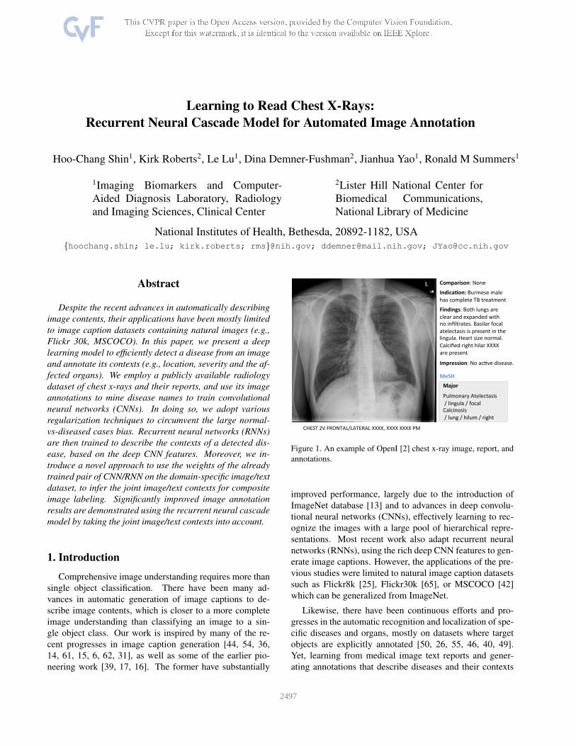
Comparison:"None""

Indica-on:"Burmese"male"

has"complete"TB"treatment"/

Findings:"Both"lungs"are""

clear"and"expanded"with""

no"infiltrates."Basilar"focal"

atelectasis"is"present"in"the"

lingula."Heart"size"normal."

Calcified"right"hilar"XXXX""

are"present""

Impression:"No"ac?ve"disease."

"MeSH/

Major/"

Pulmonary"Atelectasis"

"/"lingula"/"focal"

Calcinosis"

"/"lung"/"hilum"/"right"

"CHEST"2V"FRONTAL/LATERAL"XXXX,"XXXX"XXXX"PM"

Figure 1. An example of OpenI [2] chest x-ray image, report, and

annotations.

improved performance, largely due to the introduction of

ImageNet database [13] and to advances in deep convolu-

tional neural networks (CNNs), effectively learning to rec-

ognize the images with a large pool of hierarchical repre-

sentations. Most recent work also adapt recurrent neural

networks (RNNs), using the rich deep CNN features to gen-

erate image captions. However, the applications of the pre-

vious studies were limited to natural image caption datasets

such as Flickr8k [25], Flickr30k [65], or MSCOCO [42]

which can be generalized from ImageNet.

Likewise, there have been continuous efforts and pro-

gresses in the automatic recognition and localization of spe-

cific diseases and organs, mostly on datasets where target

objects are explicitly annotated [50, 26, 55, 46, 40, 49].

Yet, learning from medical image text reports and gener-

ating annotations that describe diseases and their contexts

12497

have been very limited. Nonetheless, providing a descrip-

tion of a medical image’s content similar to a radiologist

would describe could have a great impact. A person can

better understand a disease in an image if it is presented

with its context, e.g., where the disease is, how severe it is,

and which organ is affected. Furthermore, a large collec-

tion of medical images can be automatically annotated with

the disease context and the images can be retrieved based

on their context, with queries such as “find me images with

pulmonary disease in the upper right lobe”.

In this work, we demonstrate how to automatically an-

notate chest x-rays with diseases along with describing the

contexts of a disease, e.g., location, severity, and the af-

fected organs. A publicly available radiology dataset is ex-

ploited which contains chest x-ray images and reports pub-

lished on the Web as a part of the OpenI [2] open source

literature and biomedical image collections. An example

of a chest x-ray image, report, and annotations available on

OpenI is shown in Figure 1.

A common challenge in medical image analysis is the

data bias. When considering the whole population, diseased

cases are much rarer than healthy cases, which is also the

case in the chest x-ray dataset used. Normal cases account

for 37% (2,696 images) of the entire dataset (7,284 im-

ages), compared to the most frequent disease1 case “opac-

ity” which accounts for 12% (840 images) and the next fre-

quent “cardiomegaly” constituting for 9% (655 images). In

order to circumvent the normal-vs-diseased cases bias, we

adopt various regularization techniques in CNN training.

In analogy to the previous works using ImageNet-trained

CNN features for image encoding and RNNs to generate

image captions, we first train CNN models with one disease

label per chest x-ray inferred from image annotations, e.g.,

“calcified granuloma”, or “cardiomegaly”. However, such

single disease labels do not fully account for the context of

a disease. For instance, “calcified granuloma in right up-

per lobe” would be labeled the same as the “small calcified

granuloma in left lung base” or “multiple calcified granu-

loma”.

Inspired by the ideas introduced in [28, 64, 27, 62, 60],

we employ the already trained RNNs to obtain the context

of annotations, and recurrently use this to infer the image

labels with contexts as attributes. Then we re-train CNNs

with the obtained joint image/text contexts and generate an-

notations based on the new CNN features. With this recur-

rent cascade model, image/text contexts are taken into ac-

count for CNN training (images with “calcified granuloma

in right upper lobe” and “small calcified granuloma in left

lung base” will be assigned different labels), to ultimately

generate better and more accurate image annotations.

1Clinical findings, disorders, and other abnormal artifacts will be col-

lectively referred to as diseases in this paper.

2. Related Work

This work was initially inspired by the early work in

image caption generation [39, 17, 16], where we take

more recently introduced ideas of using CNNs and RNNs

[44, 54, 36, 14, 61, 15, 6, 62, 31] to combine recent ad-

vances in computer vision and machine translation. We

also exploit the concepts of leveraging the mid-level RNN

representations to infer image labels from the annotations

[28, 64, 27, 62, 60].

Methods for mining and predicting labels from radiology

images and reports were investigated in [51, 52, 57]. How-

ever, the image labels were mostly limited to disease names

and did not contain much contextual information. Further-

more, the majority of cases in the datasets were diseased

cases. In reality, most cases are normal, so that it is a chal-

lenge to detect relatively rarer diseased cases within such

unbalanced data.

Mining images and image labels from a large collections

of photo streams and blog posts on the Web were demon-

strated in [34, 33, 35] where images could be searched with

natural language queries. Associating neural word embed-

dings and deep image representations were explored in [37],

but generating descriptions from such images/text pairs or

image/word embeddings have not yet been demonstrated.

Detecting diseases from x-rays was demonstrated in

[3, 45, 29], classifying chest x-ray image views in [63], and

segmenting body parts in chest x-rays and computed tomog-

raphy in [5, 21]. However, learning image contexts from

text and re-generating image descriptions similar to what a

human would describe have not yet been studied. To the

best of our knowledge, this is the first study mining from a

radiology image and report dataset, not only to classify and

detect images but also to describe their context.

3. Dataset

We use a publicly available radiology dataset of chest x-

rays and reports that is a subset of the OpenI [2] open source

literature and biomedical image collections. It contains

3,955 radiology reports from the Indiana Network for Pa-

tient Care, and 7,470 associated chest x-rays from the hospi-

tals’ picture archiving systems. The entire dataset has been

fully anonymized via an aggressive anonymization scheme,

which achieved 100% precision in de-identification. How-

ever, a few findings have been rendered uninterpretable.

More details about the dataset and the anonymization pro-

cedure can be found in [11], and an example case of the

dataset is shown in Figure 1.

Each report is structured as comparison, indication, find-

ings, and impression sections, in line with a common radi-

ology reporting format for diagnostic chest x-rays. In the

example shown in Figure 1, we observe an error resulting

from the aggressive automated de-identification scheme. A

2498

MeSH Term Total Overlap Overlap Percent

normal 2,696 0 0%

opacity 840 666 79%

cardiomegaly 655 492 75%

calcinosis 558 444 80%

lung/hypoinflation 539 361 67%

calcified granuloma 511 303 59%

thoracic vertebrae/degenerative 471 296 63%

lung/hyperdistention 400 260 65%

spine/degenerative 337 219 65%

catheters, indwelling 222 159 72%

granulomatous disease 213 165 78%

nodule 211 160 76%

surgical instruments 180 120 67%

Table 1. Thirteen most frequent MeSH terms appearing over 180

times, and the number of the terms mentioned with other terms

(overlap) in an image and their percentages.

word possibly indicating a disease was falsely detected as

a personal information, and was thereby “anonymized” as

“XXXX”. While radiology reports contain comprehensive

information about the image and the patient, they may also

contain information that cannot be inferred from the image

content. For instance, in the example shown in Figure 1, it

is probably impossible to determine that the image is of a

Burmese male.

On the other hand, a manual annotation of MEDLINE R©

citations with controlled vocabulary terms (Medical Subject

Headings (MeSH R©) [1]) is known to significantly improve

the quality of the image retrieval results [20, 22, 10]. MeSH

terms for each radiology report in OpenI (available for pub-

lic use) are annotated according to the process described in

[12]. We use these to train our model.

Nonetheless, it is impossible to assign a single image la-

bel based on MeSH and train a CNN to reproduce them,

because MeSH terms seldom appear individually when de-

scribing an image. The twenty most frequent MeSH terms

appear with other terms in more than 60% of the cases. Nor-

mal cases (term “normal”) on the contrary, do not have any

overlap, and account for 37% of the entire dataset. The thir-

teen most frequent MeSH terms appearing more than 180

times are provided in Table 1, along with the total number of

cases in which they appear, the number of cases they over-

lap with in an image and the overlap percentages. The x-ray

images are provided in Portable Network Graphics (PNG)

format, with sizes varying from 512×420 to 512×624. We

rescale all CNN input training and testing images to a size

of 256× 256.

4. Disease Label Mining

The CNN-RNN based image caption generation ap-

proaches [44, 54, 36, 14, 61, 15, 6, 62, 31] require a well-

trained CNN to encode input images effectively. Unlike

natural images that can simply be encoded by ImageNet-

trained CNNs, chest x-rays differ significantly from the Im-

ageNet images. In order to train CNNs with chest x-ray

images, we sample some frequent annotation patterns with

less overlaps for each image, in order to assign image labels

to each chest x-ray image and train with cross-entropy crite-

ria. This is similar to the previous works from [51, 52, 57],

which mines disease labels of images from their annotation

text (radiology reports).

We find 17 unique patterns of MeSH term combina-

tions appearing in 30 or more cases. This allows us

to split the dataset in training/validation/testing cases as

80%/10%/10% and place at least 10 cases each in the val-

idation and testing sets. They include the terms shown in

Table 1, as well as scoliosis, osteophyte, spondylosis, frac-

tures/bone. MeSH terms appearing frequently but with-

out unique appearance patterns include pulmonary atelec-

tasis, aorta/tortuous, pleural effusion, cicatrix, etc. They

often appear with other disease terms (e.g. consolidation,

airspace disease, atherosclerosis). We retain about 40% of

the full dataset with this disease image label mining, where

the annotations for the remaining 60% of images are more

complex (and it is therefore difficult to assign a single dis-

ease label).

5. Image Classification with CNN

We use the aforementioned 17 unique disease annotation

patterns (in Table 1, and scoliosis, osteophyte, spondylosis,

fractures/bone) to label the images and train CNNs. For

this purpose, we adopt various regularization techniques to

deal with the normal-vs-diseased cases bias. For our default

CNN model we chose the simple yet effective Network-In-

Network (NIN) [41] model because the model is small in

size, fast to train, and achieves similar or better performance

to the most commonly used AlexNet model [38]. We then

test whether our data can benefit from a more complex state-

of-the-art CNN model, i.e. GoogLeNet [58].

From the 17 chosen disease annotation patterns, normal

cases account for 71% of all images, well above the num-

bers of cases for the remaining 16 disease annotation pat-

terns. We balance the number of samples for each case by

augmenting the training images of the smaller cases where

we randomly crop 224× 224 size images from the original

256× 256 size image.

5.1. Regularization by Batch Normalization andData Dropout

Even when we balance the dataset by augmenting many

diseased samples, it is difficult for a CNN to learn a good

model to distinguish many diseased cases from normal

cases which have many variations on their original samples.

It was shown in [27] that normalizing via mini-batch statis-

tics during training can serve as an effective regularization

technique to improve the performance of a CNN model. By

2499

training accuracy validation accuracy

NIN with batch-normalization (BN) 94.06% 56.65%

NIN with data-dropout (DDropout) 98.78% 58.38%

NIN with BN and DDropout 100.0% 62.43%

Table 2. Training and validation accuracy of NIN model with

batch-normalization, data-dropout, and both. Diseased cases are

very limited compared to normal cases, leading to overfitting even

with regularizations.

training accuracy validation accuracy

GoogLeNet with BN and DDropout 98.11% 66.40%

GoogLeNet with BN, DDropout, No-Crop 100.0% 69.84%

Table 3. Training and validation accuracy of GoogLeNet model

with batch-normalization, data-dropout, and without cropping the

images for data augmentation.

normalizing via mini-batch statistics, the training network

was shown not to produce deterministic values for a given

training example, thereby regularizing the model to gener-

alize better.

Inspired by this and by the concept of Dropout [23], we

regularize the normal-vs-diseased cases bias via randomly

dropping out an excessive proportion of normal cases com-

pared to the frequent diseased pattern when sampling mini-

batches. We then normalize according to the mini-batch

statistics where each mini-batch consists of a balanced num-

ber of samples per disease case and a random selection

of normal case samples. The number of samples for dis-

ease cases is balanced by random cropping during training,

where each image of a diseased case is augmented at least

four times.

We test both regularization techniques to assess their ef-

fectiveness on our dataset. The training and validation ac-

curacies of the NIN model with batch-normalization, data-

dropout, and both are provided in Table 2. While batch-

normalization and data-dropout alone do not significantly

improve performance, combining both increases the valida-

tion accuracy by about 2%.

5.2. Effect of Model Complexity

We also validate whether the dataset can benefit from

a more complex GoogLeNet [58], which is arguably the

current state-of-the-art CNN architecture. We apply both

batch-normalization and data-dropout, and follow recom-

mendations suggested in [27] (where human accuracy on

the ImageNet dataset is superseded): increase learning rate,

remove dropout, remove local response normalization. The

final training and validation accuracies using GoogLeNet

model are provided in Table 3, where we achieve a higher

(∼ 4%) accuracy2. We also observe a further ∼ 3% in-

2The final models are trained with default learning rate of 1.0, with

step down learning rate scheduling decreasing the learning rate by 50% and

33% each for NIN and GoogLeNet model in every 1/3th of the total 100

IN

h!~"

i!(input!gate)!

h!

f (forget!gate)!

o

(output!g

ate)!

OUT

(a) Long Short-Term Memory RNN

h!~" h!

OUT

IN

z (update!gate)!

r (reset!gate)!

(b) Gated Recurrent Unit RNN

Figure 2. Simplified illustrations of (a) Long Short-Term Memory

(LSTM) and (b) Gated Recurrent Unit (GRU) RNNs. The illustra-

tions are adapted and modified from Figure 2 in [8].

crease in accuracy when the images are no longer cropped,

but merely duplicated to balance the dataset.

6. Annotation Generation with RNN

We use recurrent neural networks (RNNs) to learn the

annotation sequence given input image CNN embeddings.

We test both Long Short-Term Memory (LSTM) [24] and

Gated Recurrent Unit (GRU) [7] implementations of RNNs.

Simplified illustrations of LSTM and GRU are shown in

Figure 2, and the details of both RNN implementations are

briefly introduced below.

6.1. Recurrent Neural Network Implementations

Long Short-Term Memory The LSTM implementation,

originally proposed in [24], has been successfully applied to

speech recognition [19], sequence generation [18], machine

translation [7, 56, 43], and several image caption generation

works mentioned in the main paper. LSTM is defined by the

following equations:

it = σ(W (i)xt + U (i)mt−1) (1)

ft = σ(W (f)xt + U (f)mt−1) (2)

ot = σ(W (o)xt + U (o)mt−1) (3)

ht = tanh(W (h)xt + U (h)mt−1) (4)

ht = ft ⊙ ht−1 + it ⊙ ht (5)

mt = ot ⊙ tanh(ht) (6)

where it is the input gate, ft the forget gate, ot the output

gate, ht the state vector (memory), ht the new state vector

(new memory), and mt the output vector. W is a matrix of

trained parameters (weights), and σ is the logistic sigmoid

training epochs. We could not achieve high enough validation accuracy

using exponential learning rate decay as in [27].

2500

function. ⊙ represents the product of a vector with a gate

value.

Please note that the notation used for the memory (ht, ht)

and output (mt) vectors differs from that in [24] and the

other previous work. Our notation is intended to simplify

the annotations and figures comparing LSTM to GRU.

Gated Recurrent Unit The GRU implementation has

been proposed most recently in [7], where it was success-

fully applied to machine translation. GRU is defined by the

following equations:

zt = σ(W (z)xt + U (z)ht−1) (7)

rt = σ(W (r)xt + U (r)ht−1) (8)

ht = tanh(Wxt + rt ⊙ Uht−1) (9)

ht = zt ⊙ ht−1 + (1− zt)⊙ ht (10)

where zt is the update gate, rt the reset gate, ht the new

state vector, and ht the final state vector.

6.2. Training

The number of MeSH terms describing diseases ranges

from 1 to 8 (except normal which is one word), with a mean

of 2.56 and standard deviation of 1.36. The majority of de-

scriptions contain up to five words. Since only 9 cases have

images with descriptions longer than 6 words, we ignore

these by constraining the RNNs to unroll up to 5 time steps.

We zero-pad annotations with less than five words with the

end-of-sentence token to fill in the five word space.

The parameters of the gates in LSTM and GRU decide

whether to update their current state h to the new candi-

date state h, where these are learned from the previous in-

put sequences. Further details about LSTM can be found

in [24, 15, 14, 61], and about GRU and its comparisons to

LSTM in [7, 30, 9, 8, 32]. We set the initial state of RNNs

as the CNN image embedding (CNN(I)), and the first an-

notation word as the initial input. The output of the RNNs

are the following annotation word sequences, and we train

RNNs by minimizing the negative log likelihood of output

sequences and true sequences:

L(I, S) = −N∑

t=1

{PRNN(yt = st)|CNN(I)}, (11)

where yt is the output word of RNN in time step t, st the

correct word, CNN(I) the CNN embedding of input image

I , and N the number of words in the annotation (N = 5with the end-of-sequence zero-padding). Equation 11 is not

a true conditional probability (because we only initialize the

train validation test

BLEU -1/ -2/ -3 / -4 BLEU -1/ -2/ -3 / -4 BLEU -1/ -2/ -3 / -4

LSTM 82.6 / 19.2 / 2.2 / 0.0 67.4 / 15.1 / 1.6 / 0.0 78.3 / 0.4 / 0.0 / 0.0

GRU 98.9 / 46.9 / 1.2 / 0.0 85.8 / 14.1 / 0.0 / 0.0 75.4 / 3.0 / 0.0 / 0.0

Table 4. BLEU scores validated on the training, validation, test set,

using LSTM and GRU RNN models for the sequence generation.

RNNs’ state vector to be CNN(I)) but a convenient way to

describe the training procedure.

Unlike the previous work [31, 15, 14] where they use

the last (FC-8) or second last (FC-7) fully-connected lay-

ers of AlexNet [38] or VGG-Net [53] model, the NIN or

GoogLeNet models replace the fully-connected layers with

the average-pooling layers [41, 58]. We therefore use the

output of the last spatial average-pooling layer as the image

embedding to initialize the RNN state vectors. The size of

our RNNs’ state vectors are R1×1024, which is identical to

the output size of the average-pooling layers from NIN and

GoogLeNet.

6.3. Sampling

In sampling we again initialize the RNN state vectors

with the CNN image embedding (ht=1=CNN(I)). We then

use the CNN prediction of the input image as the first word

as the input to the RNN, to sample following sequences up

to five words. As previously, images are normalized by

the batch statistics before being fed to the CNN. We use

GoogLeNet as our default CNN model since it performs

better than the NIN model in Sec. 5.2.

6.4. Evaluation

We evaluate the annotation generation on the BLEU [47]

score averaged over all of the images and their annotations

in the training, validation, and test set. BLEU scores is a

metric measuring a modified form of precision to compare

n-gram words of generated and reference sentences. The

BLEU scores evaluated are provided in Table 4. The BLEU-

N scores are evaluated for cases with ≥ N words in the

annotations, using the implementation of [4].

We noticed that LSTM is easier to train, while GRU

model yields better results with more carefully selected

hyper-parameters3. While we find it difficult to conclude

which model is better, the GRU model seems to achieve

higher scores on average.

3The final LSTM models are obtained with – learning rate: 2× 10−3,

learning rate decay: 0.97, decay rate: 0.95, without dropout; and the final

GRU model is obtained with – learning rate: 1×10−4, learning rate decay:

0.99, decay rate: 0.99, with dropout rate: 0.9. With the same setting,

adding dropout to LSTM model has adverse effect on its validation loss,

similarly when increasing the number of LSTM layers to 3. The number

of layers are 2 for both RNN models, and they are both trained with the

batch size of 50.

2501

image"input (I)

CNN"

CNN(I)

= C

NN

(I) h!t=1!

h!~"

word"

initialize

RNN"

IN 1"

OUT word"2"

h!

word"

RNN"

2"

OUT word"3"

IN

t=2!

h!

word"

RNN"

NS1"

OUT word"N"

t=N!

IN

…/t=1" h!

~"t=2" h!

~"t=N"

unroll unroll

mean"pooling"

joint"image/text"context"vector:" h!IM:TEXT!

Figure 3. An illustration of how joint image/text context vector is obtained. RNN’s state vector (h) is initialized with the CNN image

embedding (CNN(I)), and it’s unrolled over the annotation sequences with the words as input. Mean-pooling is applied over the state

vectors in each word of the sequence, to obtain the joint image/text context vector. All RNNs share the same parameters, which are trained

in the first round.

7. Recurrent Cascade Model for Image Label-

ing with Joint Image/Text Context

In Section 5, our CNN models are trained with disease

labels only where the context of diseases are not considered.

For instance, the same calcified granuloma label is assigned

to all image cases that actually may describe the disease dif-

ferently in a finer semantic level, such as “calcified granu-

loma in right upper lobe”, “small calcified granuloma in left

lung base”, and “multiple calcified granuloma”.

Meanwhile, the RNNs trained in Section 6 encode the

text annotation sequences given the CNN embedding of the

image the annotation is describing. We therefore use the al-

ready trained CNN and RNN to infer better image labels,

integrating the contexts of the image annotations beyond

just the name of the disease. This is achieved by generating

joint image/text context vectors that are computed by apply-

ing mean-pooling on the state vectors (h) of RNN at each

step over the annotation sequence. Note, that the state vec-

tor of RNN is initialized with the CNN image embeddings

(CNN(I)), and the RNN is unrolled over the annotation se-

quence, taking each word of the annotation as input. The

procedure is illustrated in Figure 3, and the RNNs share the

same parameters.

The obtained joint image/text context vector (him:text) en-

codes the image context as well as the text context describ-

ing the image. Using a notation similar to Equation 11, the

joint image/text context vector can be written as:

him:text =

∑N

t=1{hRNN(xt)|CNN(I)}

N, (12)

where xt is the input word in the annotation sequence with

N words. Different annotations describing a disease are

thereby separated into different categories by the him:text,

as shown in Figure 4. In Figure 4, the him:text vectors of

about fifty annotations describing calcified granuloma are

projected onto two-dimensional planes via dimensionality

reduction (R1×1024 → R1×2), using the t-SNE [59] imple-

mentation of [48]. We use the GRU implementation of the

RNN because it showed better overall BLEU scores in Table

4. A visualization example for the annotations describing

opacity can be found in the supplementary material.

From the him:text generated for each of the im-

age/annotation pair in the training and validation sets, we

obtain new image labels taking disease context into account.

In addition, we are no longer limited to disease annotation

mostly describing a single disease. The joint image/text

context vector him:text summarizes both the image’s context

and word sequence, so that annotations such as “calcified

granuloma in right upper lobe”, “small calcified granuloma

in left lung base”, and “multiple calcified granuloma” have

different vectors based on their contexts.

Additionally, disease labels used in Section 5 with

unique annotation patterns now have more cases, as cases

with a disease described by different annotation words are

no longer filtered out. For example, calcified granuloma

previously had only 139 cases because cases with multiple

2502

Figure 4. Visualization of joint image/text context vectors of about

50 samples of the annotations describing disease calcified gran-

uloma on 2D planes. Dimension reduction (R1×1024 → R1×2)

is performed using t-SNE [59]. Annotations describing a same

disease can be divided into different “labels” based on their joint

image/text contexts.

diseases mentioned or with long description sequences were

filtered out. At present, 414 cases are associated with cal-

cified granuloma. Likewise, opacity now has 207 cases, as

opposed to the previous 65. The average number of cases

all first-mentioned disease labels has is 83.89, with a stan-

dard deviation of 86.07, a maximum of 414 (calcified gran-

uloma) and a minimum of 18 (emphysema).

For a disease label having more than 170 cases (n ≥170 = (average+standard deviation)), we divide the cases

into sub-groups of more than 50 cases by applying k-means

clustering to the him:text vector with k = Round(n/50). We

train the CNN once more with the additional labels (57,

compared to 17 in Section 5), train the RNN with the new

CNN image embedding, and finally generate image anno-

tations. The new RNN training cost function (compared to

Equation 11) can be expressed as:

L(I, S) =

−N∑

t=1

[PRNNiter=1(yt = st) | {CNNiter=1(I)|him:textiter=0

}] ,

(13)

where him:textiter=0denotes the joint image/text context vec-

tor obtained from the first round (with limited cases and im-

…"

…"

…"

…"

…"

…"

…"

."."

CNN"

calcified""

granuloma"/""

lung"/"le3"

images"

annota6ons"

calcified""

granuloma"

lung"RNN"

RNN"

train"CNN"to"

detect"objects"

(17"object"labels)"

train"RNN"to"

describe"their"

contexts"

mean"pooling"

joint"im

age/text"

context"vectors"

1. 

ini6al"training"of"CNN/RNN"

"""""""with"single"object"labels"

calcified""

granuloma"/""

lung"/"le3"

images"

annota6ons"

CNN"

RNN"

RNN"

2."compute"labels"based"on""

""""joint"im

age/text"contexts"

reFuse""

trained"

CNN/RNN"

weights"

calcified(granuloma(…(le0(m

ul1ple(

calcified(granuloma(…(spine(…(

calcified(granuloma(…(small(

calcified(granuloma(

calcified(granuloma(…(vertabrae(…(

calcified(granuloma(…(lung(lower(lobe(…(

calcified(granuloma(…(m

iddle(lobe(…(

calcified(granuloma(…(bilateral(mul1ple(

calcified""

granuloma"/""

…"/"spine"…"

images"

annota6ons"

CNN"

RNN"

RNN"

reFtrain"

CNN/RNN"

fineFtuning"

the"weights"

spine"

le3"

joint"context"

label"x"

lung"

calcified""

granuloma"

train"CNN"to"

detect"objects"

with"context"

the"first"object""

for"annota6on"

train"RNN"to"

describe"their"

contexts"and""

other"object""

and"context"

if"any"

assign"joint"text/image"

context"labels"by"clustering"

3."training"CNN/RNN"with""

""""joint"im

age/text"context"labels"

training"subset"(40%)"with"single"object""

en6re"training"set""

en6re"training"set""

(57"context"

labels)"

Figure 5. Overall workflow for the automated image annotation.

age labels at 0th iteration) of CNN and RNN training. In

the second CNN training round (1st iteration), we fine-tune

from the previous CNNiter=0, by replacing the last classi-

fication layer with the new set of labels (17 → 57) and

training it with a lower learning rate (0.1), except for the

classification layer. The overall workflow is illustrated in

Figure 5.

7.1. Evaluation

The final evaluated BLEU scores are provided in Table 5.

We achieve better overall BLEU scores than those in Table

4 before using the joint image/text context. It is noticeable

that higher BLEU-N (N > 1) scores are achieved com-

pared to Table 4, indicating that more comprehensive image

contexts are taken into account for the CNN/RNN training.

Also, slightly better BLEU scores are obtained using GRU

on average and higher BLEU-1 scores are acquired using

LSTM, although the comparison is empirical. Examples of

2503

opacity///lung///middle_lobe///

right//aorta_thoracic///tortuous/

opacity///lung///base///leA/

opacity///lung///middle_lobe///

right///blood_vessels/

calcified_granuloma///lung///

middle_lobe///right/

calcified_granuloma///lung///

middle_lobe///right///mul-ple/

calcified_granuloma///lung///

hilum///right/

airspace_disease///lung///hilum///

right///lung///hilum/

nodule///lung///hilum///right/

input/im

age/

generated/annota-on/

true/annota-on/

aorta_thoracic///tortuous///mild/

aorta_thoracic///tortuous/

thoracic_vertebrae_degenera-ve/

//mild/

aorta_tortuous//

thoracic_vertebrae_degenera-ve/

//mild/

normal/

normal/

normal/

normal/

Figure 6. Examples of annotation generations (light green box) compared to true annotations (yellow box) for input images in the test set.

train validation test

BLEU -1/ -2/ -3 / -4 BLEU -1/ -2/ -3 / -4 BLEU -1/ -2/ -3 / -4

LSTM 97.2 / 67.1 / 14.9 / 2.8 68.1 / 30.1 / 5.2 / 1.1 79.3 / 9.1 / 0.0 / 0.0

GRU 89.7 / 61.7 / 28.5 / 11.0 61.9 / 29.6 / 11.3 / 2.0 78.5 / 14.4 / 4.7 / 0.0

Table 5. BLEU scores validated on the training, validation, test set,

using LSTM and GRU RNN models trained on the first iteration,

for the sequence generation.

generated annotations on the chest x-ray images are shown

in Figure 6. These are generated using the GRU model, and

more examples can be found in the supplementary material.

8. Conclusion

We present an effective framework to learn, detect dis-

ease, and describe their contexts from the patient chest x-

rays and their accompanying radiology reports with Med-

ical Subject Headings (MeSH) annotations. Furthermore,

we introduce an approach to mine joint contexts from a col-

lection of images and their accompanying text, by summa-

rizing the CNN/RNN outputs and their states on each of the

image/text instances. Higher performance on text genera-

tion is achieved on the test set if the joint image/text con-

texts are exploited to re-label the images and to train the

proposed CNN/RNN framework subsequently.

To the best of our knowledge, this is the first study that

mines from a publicly available radiology image and report

dataset, not only to classify and detect disease in images

but also to describe their context similar to a human ob-

server would read. While we only demonstrate on a med-

ical dataset, the suggested approach could also be applied

to other application scenario with datasets containing co-

existing pairs of images and text annotations, where the

domain-specific images differ from those of the ImageNet.

Acknowledgement

This work was supported in part by the Intramural Re-

search Program of the National Institutes of Health Clin-

ical Center, and in part by a grant from the KRIBB Re-

search Initiative Program (Korean Biomedical Scientist Fel-

lowship Program), Korea Research Institute of Bioscience

and Biotechnology, Republic of Korea. We thank NVIDIA

for the K40 GPU donation.

2504

References

[1] Mesh: Medical subject headings. https://www.nlm.

nih.gov/mesh/meshhome.html.

[2] Open-i: An open access biomedical search engine. https:

//openi.nlm.nih.gov.

[3] U. Avni, H. Greenspan, E. Konen, M. Sharon, and J. Gold-

berger. X-ray categorization and retrieval on the organ and

pathology level, using patch-based visual words. Medical

Imaging, IEEE Transactions on, 2011.

[4] S. Bird, E. Klein, and E. Loper. Natural language processing

with Python. ” O’Reilly Media, Inc.”, 2009.

[5] H. Boussaid and I. Kokkinos. Fast and exact: Admm-based

discriminative shape segmentation with loopy part models.

2014.

[6] X. Chen and C. Lawrence Zitnick. Mind’s eye: A recurrent

visual representation for image caption generation. In CVPR,

2015.

[7] K. Cho, B. Van Merrienboer, C. Gulcehre, D. Bahdanau,

F. Bougares, H. Schwenk, and Y. Bengio. Learning phrase

representations using rnn encoder-decoder for statistical ma-

chine translation. arXiv preprint arXiv:1406.1078, 2014.

[8] J. Chung, C. Gulcehre, K. Cho, and Y. Bengio. Empirical

evaluation of gated recurrent neural networks on sequence

modeling. arXiv preprint arXiv:1412.3555, 2014.

[9] J. Chung, C. Gulcehre, K. Cho, and Y. Bengio. Gated

feedback recurrent neural networks. arXiv preprint

arXiv:1502.02367, 2015.

[10] S. J. Darmoni, L. F. Soualmia, C. Letord, M.-C. Jaulent,

N. Griffon, B. Thirion, and A. Neveol. Improving informa-

tion retrieval using medical subject headings concepts: a test

case on rare and chronic diseases. Journal of the Medical

Library Association: JMLA, 100(3):176, 2012.

[11] D. Demner-Fushman, M. D. Kohli, M. B. Rosenman, S. E.

Shooshan, L. Rodriguez, S. Antani, G. R. Thoma, and C. J.

McDonald. Preparing a collection of radiology examinations

for distribution and retrieval. Journal of the American Medi-

cal Informatics Association, page ocv080, 2015.

[12] D. Demner-Fushman, S. E. Shooshan, L. Rodriguez, S. An-

tani, and G. R. Thoma. Annotation of chest radiology reports

for indexing and retrieval. Multimodal Retrieval in the Med-

ical Domain (MRMD) 2015.

[13] J. Deng, W. Dong, R. Socher, L.-J. Li, K. Li, and L. Fei-

Fei. Imagenet: A large-scale hierarchical image database. In

CVPR, 2009.

[14] J. Donahue, L. Anne Hendricks, S. Guadarrama,

M. Rohrbach, S. Venugopalan, K. Saenko, and T. Dar-

rell. Long-term recurrent convolutional networks for visual

recognition and description. In CVPR, 2015.

[15] H. Fang, S. Gupta, F. Iandola, R. K. Srivastava, L. Deng,

P. Dollar, J. Gao, X. He, M. Mitchell, J. C. Platt, et al. From

captions to visual concepts and back. In CVPR, 2015.

[16] A. Farhadi, M. Hejrati, M. A. Sadeghi, P. Young,

C. Rashtchian, J. Hockenmaier, and D. Forsyth. Every pic-

ture tells a story: Generating sentences from images. In

ECCV. 2010.

[17] Y. Feng and M. Lapata. How many words is a picture worth?

automatic caption generation for news images. In Proceed-

ings of the 48th annual meeting of the Association for Com-

putational Linguistics, 2010.

[18] A. Graves. Generating sequences with recurrent neural net-

works. arXiv preprint arXiv:1308.0850, 2013.

[19] A. Graves, A.-r. Mohamed, and G. Hinton. Speech recog-

nition with deep recurrent neural networks. In Acoustics,

Speech and Signal Processing (ICASSP), 2013 IEEE Inter-

national Conference on. IEEE, 2013.

[20] R. B. Haynes, N. Wilczynski, K. A. McKibbon, C. J. Walker,

and J. C. Sinclair. Developing optimal search strategies for

detecting clinically sound studies in medline. Journal of the

American Medical Informatics Association, 1(6):447, 1994.

[21] S. Hermann. Evaluation of scan-line optimization for 3d

medical image registration. In CVPR, 2014.

[22] W. Hersh and E. Voorhees. Trec genomics special issue

overview. Information Retrieval, 12(1):1–15, 2009.

[23] G. E. Hinton, N. Srivastava, A. Krizhevsky, I. Sutskever, and

R. R. Salakhutdinov. Improving neural networks by pre-

venting co-adaptation of feature detectors. arXiv preprint

arXiv:1207.0580, 2012.

[24] S. Hochreiter and J. Schmidhuber. Long short-term memory.

Neural computation, 9(8):1735–1780, 1997.

[25] M. Hodosh, P. Young, and J. Hockenmaier. Framing image

description as a ranking task: Data, models and evaluation

metrics. Journal of Artificial Intelligence Research, 2013.

[26] J. Hofmanninger and G. Langs. Mapping visual features to

semantic profiles for retrieval in medical imaging. In CVPR,

2015.

[27] S. Ioffe and C. Szegedy. Batch normalization: Accelerating

deep network training by reducing internal covariate shift.

arXiv preprint arXiv:1502.03167, 2015.

[28] O. Irsoy and C. Cardie. Opinion mining with deep recur-

rent neural networks. In Proceedings of the 2014 Confer-

ence on Empirical Methods in Natural Language Processing

(EMNLP), 2014.

[29] S. Jaeger, A. Karargyris, S. Candemir, L. Folio, J. Siegelman,

F. Callaghan, Z. Xue, K. Palaniappan, R. K. Singh, S. Antani,

et al. Automatic tuberculosis screening using chest radio-

graphs. Medical Imaging, IEEE Transactions on, 2014.

[30] R. Jozefowicz, W. Zaremba, and I. Sutskever. An empiri-

cal exploration of recurrent network architectures. In ICML

2015, 2015.

[31] A. Karpathy and L. Fei-Fei. Deep visual-semantic align-

ments for generating image descriptions. In CVPR, 2015.

[32] A. Karpathy, J. Johnson, and F.-F. Li. Visualizing

and understanding recurrent networks. arXiv preprint

arXiv:1506.02078, 2015.

[33] G. Kim, S. Moon, and L. Sigal. Joint photo stream and blog

post summarization and exploration. In CVPR, 2015.

[34] G. Kim, S. Moon, and L. Sigal. Ranking and retrieval of

image sequences from multiple paragraph queries. In CVPR,

2015.

[35] G. Kim, L. Sigal, and E. P. Xing. Joint summarization of

large-scale collections of web images and videos for story-

line reconstruction. In CVPR, 2014.

2505

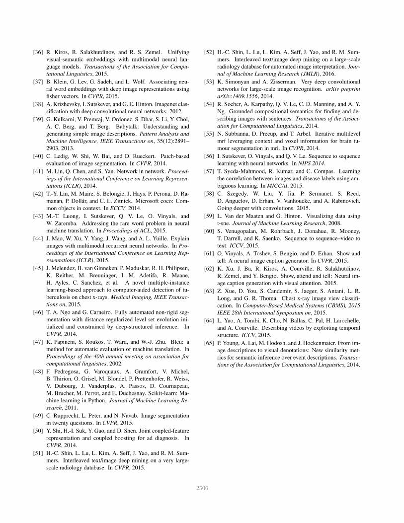
[36] R. Kiros, R. Salakhutdinov, and R. S. Zemel. Unifying

visual-semantic embeddings with multimodal neural lan-

guage models. Transactions of the Association for Compu-

tational Linguistics, 2015.

[37] B. Klein, G. Lev, G. Sadeh, and L. Wolf. Associating neu-

ral word embeddings with deep image representations using

fisher vectors. In CVPR, 2015.

[38] A. Krizhevsky, I. Sutskever, and G. E. Hinton. Imagenet clas-

sification with deep convolutional neural networks. 2012.

[39] G. Kulkarni, V. Premraj, V. Ordonez, S. Dhar, S. Li, Y. Choi,

A. C. Berg, and T. Berg. Babytalk: Understanding and

generating simple image descriptions. Pattern Analysis and

Machine Intelligence, IEEE Transactions on, 35(12):2891–

2903, 2013.

[40] C. Ledig, W. Shi, W. Bai, and D. Rueckert. Patch-based

evaluation of image segmentation. In CVPR, 2014.

[41] M. Lin, Q. Chen, and S. Yan. Network in network. Proceed-

ings of the International Conference on Learning Represen-

tations (ICLR), 2014.

[42] T.-Y. Lin, M. Maire, S. Belongie, J. Hays, P. Perona, D. Ra-

manan, P. Dollar, and C. L. Zitnick. Microsoft coco: Com-

mon objects in context. In ECCV. 2014.

[43] M.-T. Luong, I. Sutskever, Q. V. Le, O. Vinyals, and

W. Zaremba. Addressing the rare word problem in neural

machine translation. In Proceedings of ACL, 2015.

[44] J. Mao, W. Xu, Y. Yang, J. Wang, and A. L. Yuille. Explain

images with multimodal recurrent neural networks. In Pro-

ceedings of the International Conference on Learning Rep-

resentations (ICLR), 2015.

[45] J. Melendez, B. van Ginneken, P. Maduskar, R. H. Philipsen,

K. Reither, M. Breuninger, I. M. Adetifa, R. Maane,

H. Ayles, C. Sanchez, et al. A novel multiple-instance

learning-based approach to computer-aided detection of tu-

berculosis on chest x-rays. Medical Imaging, IEEE Transac-

tions on, 2015.

[46] T. A. Ngo and G. Carneiro. Fully automated non-rigid seg-

mentation with distance regularized level set evolution ini-

tialized and constrained by deep-structured inference. In

CVPR, 2014.

[47] K. Papineni, S. Roukos, T. Ward, and W.-J. Zhu. Bleu: a

method for automatic evaluation of machine translation. In

Proceedings of the 40th annual meeting on association for

computational linguistics, 2002.

[48] F. Pedregosa, G. Varoquaux, A. Gramfort, V. Michel,

B. Thirion, O. Grisel, M. Blondel, P. Prettenhofer, R. Weiss,

V. Dubourg, J. Vanderplas, A. Passos, D. Cournapeau,

M. Brucher, M. Perrot, and E. Duchesnay. Scikit-learn: Ma-

chine learning in Python. Journal of Machine Learning Re-

search, 2011.

[49] C. Rupprecht, L. Peter, and N. Navab. Image segmentation

in twenty questions. In CVPR, 2015.

[50] Y. Shi, H.-I. Suk, Y. Gao, and D. Shen. Joint coupled-feature

representation and coupled boosting for ad diagnosis. In

CVPR, 2014.

[51] H.-C. Shin, L. Lu, L. Kim, A. Seff, J. Yao, and R. M. Sum-

mers. Interleaved text/image deep mining on a very large-

scale radiology database. In CVPR, 2015.

[52] H.-C. Shin, L. Lu, L. Kim, A. Seff, J. Yao, and R. M. Sum-

mers. Interleaved text/image deep mining on a large-scale

radiology database for automated image interpretation. Jour-

nal of Machine Learning Research (JMLR), 2016.

[53] K. Simonyan and A. Zisserman. Very deep convolutional

networks for large-scale image recognition. arXiv preprint

arXiv:1409.1556, 2014.

[54] R. Socher, A. Karpathy, Q. V. Le, C. D. Manning, and A. Y.

Ng. Grounded compositional semantics for finding and de-

scribing images with sentences. Transactions of the Associ-

ation for Computational Linguistics, 2014.

[55] N. Subbanna, D. Precup, and T. Arbel. Iterative multilevel

mrf leveraging context and voxel information for brain tu-

mour segmentation in mri. In CVPR, 2014.

[56] I. Sutskever, O. Vinyals, and Q. V. Le. Sequence to sequence

learning with neural networks. In NIPS 2014.

[57] T. Syeda-Mahmood, R. Kumar, and C. Compas. Learning

the correlation between images and disease labels using am-

biguous learning. In MICCAI. 2015.

[58] C. Szegedy, W. Liu, Y. Jia, P. Sermanet, S. Reed,

D. Anguelov, D. Erhan, V. Vanhoucke, and A. Rabinovich.

Going deeper with convolutions. 2015.

[59] L. Van der Maaten and G. Hinton. Visualizing data using

t-sne. Journal of Machine Learning Research, 2008.

[60] S. Venugopalan, M. Rohrbach, J. Donahue, R. Mooney,

T. Darrell, and K. Saenko. Sequence to sequence–video to

text. ICCV, 2015.

[61] O. Vinyals, A. Toshev, S. Bengio, and D. Erhan. Show and

tell: A neural image caption generator. In CVPR, 2015.

[62] K. Xu, J. Ba, R. Kiros, A. Courville, R. Salakhutdinov,

R. Zemel, and Y. Bengio. Show, attend and tell: Neural im-

age caption generation with visual attention. 2015.

[63] Z. Xue, D. You, S. Candemir, S. Jaeger, S. Antani, L. R.

Long, and G. R. Thoma. Chest x-ray image view classifi-

cation. In Computer-Based Medical Systems (CBMS), 2015

IEEE 28th International Symposium on, 2015.

[64] L. Yao, A. Torabi, K. Cho, N. Ballas, C. Pal, H. Larochelle,

and A. Courville. Describing videos by exploiting temporal

structure. ICCV, 2015.

[65] P. Young, A. Lai, M. Hodosh, and J. Hockenmaier. From im-

age descriptions to visual denotations: New similarity met-

rics for semantic inference over event descriptions. Transac-

tions of the Association for Computational Linguistics, 2014.

2506