Learning with Mixtures of Trees

by

Marina Meila-Predoviciu

M.S. Automatic Control and Computer Science (1985)Universitatea Politehnica Bucuresti

Submitted to the Department of Electrical Engineering and Computer Sciencein partial fulfillment of the requirements for the degree of

Doctor of Philosophy

at the

MASSACHUSETTS INSTITUTE OF TECHNOLOGY

January 1999

c© Massachusetts Institute of Technology 1999

Signature of Author . . . . . . . . . . . . . . . . . . . . . . . . . . . . . . . . . . . . . . . . . . . . . . . . . . . . . . . . . . . . . . .Department of Electrical Engineering and Computer Science

January 14, 1999

Certified by. . . . . . . . . . . . . . . . . . . . . . . . . . . . . . . . . . . . . . . . . . . . . . . . . . . . . . . . . . . . . . . . . . . . . . . .Michael I. Jordan

Professor, Department of Brain SciencesThesis Supervisor

Accepted by . . . . . . . . . . . . . . . . . . . . . . . . . . . . . . . . . . . . . . . . . . . . . . . . . . . . . . . . . . . . . . . . . . . . . . .Arthur C. Smith

Chairman, Departmental Committee on Graduate Students

2

Learning with Mixtures of Treesby

Marina Meila-Predoviciu

Revised version of a thesis submitted to theDepartment of Electrical Engineering and Computer Science

on January 14, 1999, in partial fulfillment of therequirements for the degree of

Doctor of Philosophy

Abstract

One of the challenges of density estimation as it is used in machine learning is that usu-ally the data are multivariate and often the dimensionality is large. Operating with jointdistributions over multidimensional domains raises specific problems that are not encoun-tered in the univariate case. Graphical models are representations of joint densities that arespecifically tailored to address these problems. They take advantage of the (conditional)independencies between subsets of variables in the domain which they represent by meansof a graph. When the graph is sparse, graphical models provide an excellent support for hu-man intuition and allow for efficient inference algorithms. However, learning the underlyingdependence graph from data is generally NP-hard.

The purpose of this thesis is to propose and to study a class of models that admitstractable inference and learning algorithms yet is rich enough for practical applications.This class is the class of mixtures of trees models. Mixtures of trees inherit the excellentcomputational properties of tree distributions (themselves a subset of graphical models) butcombine several trees in order to augment their modeling power, thereby going beyond thestandard graphical model framework.

The thesis demonstrates the performance of the mixture of trees in density estimationand classification tasks. In the same time it deepens the understanding of the properties ofthe tree distribution as a multivariate density model. Among others, it shows that the treeclassifier implements an implicit variable selection mechanism.

Learning mixtures of trees from data is a central subject of this thesis. The learningalgorithm that is introduced here is based on the the EM and the Minimum Weight SpanningTree algorithms and is quadratic in the dimension of the domain.

This algorithm can serve as a tool for discovering hidden variables in a special butimportant class of models where, conditioned on the hidden variable, the dependenciesbetween the observed variables become sparse.

Finally, it is shown that in the case of sparse discrete data, the original learning algorithmcan be transformed in an algorithm that is jointly subquadratic and that in simulationsachieves speedups factors of up to a thousand.

Thesis Supervisor: Michael I. JordanTitle: Professor, Department of Brain Sciences

Acknowledgments

The years at MIT have been a fantastic experience and it is a joy to remember those whoconcurred in making it so and to thank those whose influence contributed to this thesis.

Michael Jordan, my thesis advisor, fostered my interest in reinforcement learning, statis-tics, graphical models, differential geometry and . . . who knows what next? He was the soulof the unforgettable “Jordan lab” and of its equally unforgettable group meetings. He sup-ported me materially and morally during all these years while giving me complete freedomin pursuing my work. In spite of this freedom, my thesis owes enormously to his inspiringinfluence. I have deeply appreciated his relentless enthusiasm for learning and deepeningone’s understanding, the high standards he set, the genuinely positive attitude enriched bya sense for beauty that is his approach to science and life.

I thank Alan Willsky and Paul Viola, the two other members of my committee, forthe interest and support they gave to this project and especially for asking just the rightquestions to make this thesis a better one. I very much hope that these discussions will becontinue. Paul suggested a direction of work which resulted in the accelerated tree learningalgorithms. The same algorithms benefited greatly from a series of very stimulating meetingswith David Karger. Eric Grimson and Alvin Drake gave me good advice from my fist dayson, Tomaso Poggio and his group “adopted” me during my last semester of studentship,Peter Dayan, to whom I should have talked more, found the time to listen to me and aninsightful comment on every subject that I could have brought up.

Quaid Morris shared my enthusiasm for trees, coded the first mixtures of trees program,did the digits and random trees experiments. David Heckerman and the Microsoft DTASgroup hosted me in Seattle for four intense months, forcing me to take a distance from thiswork that proved to be entirely to its benefit. David with Max Chickering provided codeand ran part of the Alarm experiments.

Carl de Marcken was the most insightful critic of my ideas and my writing, answeredmy questions and thought me uncountably many things I needed to know, pondered withme over dozens of problems as if they were his own and was always the first to share withme the joy of a success.

I have had countless opportunities to appreciate the quality of the education I receivedat my Alma Mater, the Polytechnic University of Bucuresti; I take this one to thank VasileBrınzanescu, Paul Flondor, Dan Iordache, Theodor Danila, Corneliu Popeea, Vlad Ionescu,Petre Stoica for everything they thought me.

I chose the thesis topic, but chance chose my officemates. I couldn’t have been luck-ier: Greg Galperin, Tommi Jaakkola, Thomas Hofmann listened to my half baked ideas,answered patiently thousands of questions and let themselves be engaged in exciting dis-cussions on every topic under the sun. They are now among my best friends and one of thereasons I find myself enriched by the years at MIT.

Finally, there is the circle of love that constantly and invisibly surrounds us with itsstrength. Gail, Butch, Paya and Natasha who welcomed me in their family. Felicia. Carl.My mother – teacher, friend and partner in adventures. My grandfather, Judge Ioan I.Predoviciu, to whose memory I dedicate this thesis.

This research was supported through the Center for Biological and Computational Learningat MIT funded in part by the National Science Foundation under contract No. ASC-92-17041.

4

Contents

1 Introduction 15

1.1 Density estimation in multidimensional domains . . . . . . . . . . . . . . . 15

1.2 Introduction by example . . . . . . . . . . . . . . . . . . . . . . . . . . . . . 16

1.3 Graphical models of conditional independence . . . . . . . . . . . . . . . . . 171.3.1 Examples of established belief network classes . . . . . . . . . . . . . 17

1.3.2 Advantages of graphical models . . . . . . . . . . . . . . . . . . . . . 20

1.3.3 Structure learning in belief networks . . . . . . . . . . . . . . . . . . 21

1.3.4 Inference and decomposable models . . . . . . . . . . . . . . . . . . 22

1.4 Why, what and where? Goal, contributions and road map of the thesis . . . 23

1.4.1 Contributions . . . . . . . . . . . . . . . . . . . . . . . . . . . . . . . 241.4.2 A road map for the reader . . . . . . . . . . . . . . . . . . . . . . . . 25

2 Trees and their properties 272.1 Tree distributions . . . . . . . . . . . . . . . . . . . . . . . . . . . . . . . . . 27

2.2 Inference, sampling and marginalization in a tree distribution . . . . . . . . 29

2.2.1 Inference. . . . . . . . . . . . . . . . . . . . . . . . . . . . . . . . . . 29

2.2.2 Marginalization . . . . . . . . . . . . . . . . . . . . . . . . . . . . . . 30

2.2.3 Sampling . . . . . . . . . . . . . . . . . . . . . . . . . . . . . . . . . 31

2.3 Learning trees in the Maximum Likelihood framework . . . . . . . . . . . . 312.3.1 Problem formulation . . . . . . . . . . . . . . . . . . . . . . . . . . . 31

2.3.2 Fitting a tree to a distribution . . . . . . . . . . . . . . . . . . . . . 32

2.3.3 Solving the ML learning problem . . . . . . . . . . . . . . . . . . . . 35

2.4 Representation capabilities . . . . . . . . . . . . . . . . . . . . . . . . . . . 36

2.5 Appendix: The Junction Tree algorithm for trees . . . . . . . . . . . . . . 36

3 Mixtures of trees 41

3.1 Representation power of mixtures of trees . . . . . . . . . . . . . . . . . . . 43

3.2 Basic operations with mixtures of trees . . . . . . . . . . . . . . . . . . . . . 443.3 Learning mixtures of trees in the ML framework . . . . . . . . . . . . . . . 45

3.3.1 The basic algorithm . . . . . . . . . . . . . . . . . . . . . . . . . . . 45

3.3.2 Running time and storage requirements . . . . . . . . . . . . . . . . 47

3.3.3 Learning mixtures of trees with shared structure . . . . . . . . . . . 48

3.3.4 Remarks on the learning algorithms . . . . . . . . . . . . . . . . . . 49

3.4 Summary and related work . . . . . . . . . . . . . . . . . . . . . . . . . . . 50

4 Learning mixtures of trees in the Bayesian framework 534.1 MAP estimation by the EM algorithm . . . . . . . . . . . . . . . . . . . . . 54

4.2 Decomposable priors for tree distributions . . . . . . . . . . . . . . . . . . . 55

4.2.1 Decomposable priors over tree structures . . . . . . . . . . . . . . . 55

4.2.2 Priors for tree parameters: the Dirichlet prior . . . . . . . . . . . . . 56

5

5 Accelerating the tree learning algorithm 615.1 Introduction . . . . . . . . . . . . . . . . . . . . . . . . . . . . . . . . . . . . 615.2 Assumptions . . . . . . . . . . . . . . . . . . . . . . . . . . . . . . . . . . . 625.3 Accelerated CL algorithms . . . . . . . . . . . . . . . . . . . . . . . . . . . . 63

5.3.1 First idea: Comparing mutual informations between binary variables 635.3.2 Second idea: computing cooccurrences in a bipartite graph data rep-

resentation . . . . . . . . . . . . . . . . . . . . . . . . . . . . . . . . 645.3.3 Putting it all together: the aCL-I algorithm and its data structures 675.3.4 Time and storage requirements . . . . . . . . . . . . . . . . . . . . . 695.3.5 The aCL-II algorithm . . . . . . . . . . . . . . . . . . . . . . . . . . 705.3.6 Time and memory requirements for aCL-II . . . . . . . . . . . . . . 72

5.4 Generalization to discrete variables of arbitrary arity . . . . . . . . . . . . . 735.4.1 Computing cooccurrences . . . . . . . . . . . . . . . . . . . . . . . . 735.4.2 Presorting mutual informations . . . . . . . . . . . . . . . . . . . . . 74

5.5 Using the aCL algorithms with EM . . . . . . . . . . . . . . . . . . . . . . . 765.6 Decomposable priors and the aCL algorithm . . . . . . . . . . . . . . . . . 765.7 Experiments . . . . . . . . . . . . . . . . . . . . . . . . . . . . . . . . . . . . 775.8 Concluding remarks . . . . . . . . . . . . . . . . . . . . . . . . . . . . . . . 805.9 Appendix: Bounding the number of lists NL . . . . . . . . . . . . . . . . . . 80

6 An Approach to Hidden variable discovery 816.1 Structure learning paradigms . . . . . . . . . . . . . . . . . . . . . . . . . . 816.2 The problem of variable partitioning . . . . . . . . . . . . . . . . . . . . . . 836.3 The tree H model . . . . . . . . . . . . . . . . . . . . . . . . . . . . . . . . . 866.4 Variable partitioning in the general case . . . . . . . . . . . . . . . . . . . . 87

6.4.1 Outline of the procedure . . . . . . . . . . . . . . . . . . . . . . . . . 876.4.2 Defining structure as simple explanation . . . . . . . . . . . . . . . . 87

6.5 Experiments . . . . . . . . . . . . . . . . . . . . . . . . . . . . . . . . . . . . 896.5.1 Experimental procedure . . . . . . . . . . . . . . . . . . . . . . . . . 896.5.2 Experiments with tree H models . . . . . . . . . . . . . . . . . . . . 896.5.3 General H models . . . . . . . . . . . . . . . . . . . . . . . . . . . . 90

6.6 Approximating the description length of a model . . . . . . . . . . . . . . . 946.6.1 Encoding a multinomial distribution . . . . . . . . . . . . . . . . . . 94

6.7 Model validation by independence testing . . . . . . . . . . . . . . . . . . . 956.7.1 An alternate independence test . . . . . . . . . . . . . . . . . . . . . 956.7.2 A threshold for mixtures . . . . . . . . . . . . . . . . . . . . . . . . . 976.7.3 Validating graphical models with hidden variables . . . . . . . . . . 99

6.8 Discussion . . . . . . . . . . . . . . . . . . . . . . . . . . . . . . . . . . . . . 101

7 Experimental results 1037.1 Recovering the structure . . . . . . . . . . . . . . . . . . . . . . . . . . . . . 103

7.1.1 Random trees, large data set . . . . . . . . . . . . . . . . . . . . . . 1037.1.2 Random bars, small data set . . . . . . . . . . . . . . . . . . . . . . 104

7.2 Density estimation experiments . . . . . . . . . . . . . . . . . . . . . . . . . 1077.2.1 Digits and digit pairs images . . . . . . . . . . . . . . . . . . . . . . 1077.2.2 The ALARM network and data set . . . . . . . . . . . . . . . . . . . 108

7.3 Classification with mixtures of trees . . . . . . . . . . . . . . . . . . . . . . 1117.3.1 Using a mixture of trees as a classifier . . . . . . . . . . . . . . . . . 111

6

7.3.2 The AUSTRALIAN data set . . . . . . . . . . . . . . . . . . . . . . 1117.3.3 The MUSHROOM data set . . . . . . . . . . . . . . . . . . . . . . . 1137.3.4 The SPLICE data set. Classification and structure discovery . . . . 1137.3.5 The single tree classifier as an automatic feature selector . . . . . . . 119

8 Conclusion 121

7

8

List of Figures

1-1 The DNA splice junction domain. . . . . . . . . . . . . . . . . . . . . . . . . 17

1-2 An example of a Bayes net (a) and of a Markov net (b) over 5 variables. . 18

1-3 Structure of the thesis . . . . . . . . . . . . . . . . . . . . . . . . . . . . . . 25

3-1 A mixture of trees with m = 3 and n = 5. Note that although b ⊥T k c | a forall k = 1, 2, 3 this does not imply in general b ⊥ c | a for the mixture. . . . . 42

3-2 A Mixture of trees with shared structure represented as a graphical model. 42

5-1 The bipartite graph representation of a sparse data set. Each edge iv means“variable v is on in data point i”. . . . . . . . . . . . . . . . . . . . . . . . . 65

5-2 The mean (full line), standard deviation and maximum (dotted line) ofKruskal algorithm steps nK over 1000 runs plotted against n log n. n rangesfrom 5 to 3000. The edge weights were sampled from a uniform distribution. 71

5-3 The aCL-II algorithm: the data structure that supplies the next weightiestcandidate edge. Vertically to the left are the variables, sorted by decreasingNu. For a given u, there are two lists: Cu, the list of variables v u, sortedin decreasing order of Iuv and (the virtual list) V0(u) sorted by decreasingNv. The maximum of the two first elements of these lists is inserted into anF-heap.The overal maximum of Iuv can then be extracted as the maximumof the F-heap. . . . . . . . . . . . . . . . . . . . . . . . . . . . . . . . . . . . 71

5-4 Real running time for the accelerated (full line) and traditional (dotted line)TreeLearn algorithm versus number of vertices n for different values of thesparsity s. . . . . . . . . . . . . . . . . . . . . . . . . . . . . . . . . . . . . 78

5-5 Number of steps of the Kruskal algorithm nK versus domain size n measuredfor the aCL-II algorithm for different values of s . . . . . . . . . . . . . . 79

6-1 The H-model (a) and a graphical model of the same distribution marginalizedover h (b). . . . . . . . . . . . . . . . . . . . . . . . . . . . . . . . . . . . . . 84

6-2 The tree H model used for training. . . . . . . . . . . . . . . . . . . . . . . 90

6-3 The models used for training: (a) S1, (b) S2. . . . . . . . . . . . . . . . . . 90

6-4 Description lengths and accuracies for models with fixed p = 2 and variablem = 2, 3, 4 learned from data generated by the tree H model in figure 6-2.For m = 3 and 4 all structures are correct. (a) general, (b) detail of theupper left corner of (a). . . . . . . . . . . . . . . . . . . . . . . . . . . . . . 91

6-5 Model structures and their scores and accuracies, as obtained by learning treeH models with m = 3 and p = 3 on 10 data sets generated from structureS1. Circles represent good structures and x’s are the bad structures. A +marks each of the 5 lowest DL models. The x-axes measure the empiricaldescription length in bits/example, the vertical axes measure the accuracy ofthe hidden variable retrieval, whose bottom line is at 0.33 . . . . . . . . . . 92

9

6-6 Model structures and their scores and accuracies, as obtained by learningtree H models with p = 3 and variable m = 2, 3, 4, 5 on a data set generatedfrom structure S1. Circles represent good structures and x’s are the badstructures. The sizes of the symbols are proportional to m. The x-axismeasures the empirical description length in bits/example, the vertical axismeasures the accuracy of the hidden variable retrieval, whose bottom line isat 0.33. Notice the decrease in DL with increasing m. . . . . . . . . . . . . 93

7-1 Eight training examples for the bars learning task. . . . . . . . . . . . . . . 104

7-2 The true structure of the probabilistic generative model for the bars data. . 105

7-3 A mixture of trees approximate generative model for the bars problem. Theinterconnection between the variables in each “bar” are arbitrary. . . . . . . 105

7-4 Test set log-likelihood on the bars learning task for different values of thesmoothing α and different m. Averages and standard deviations over 20trials. . . . . . . . . . . . . . . . . . . . . . . . . . . . . . . . . . . . . . . . 106

7-5 An example of a digit pair. . . . . . . . . . . . . . . . . . . . . . . . . . . . 107

7-6 Average log-likelihoods (bits per digit) for the single digit (a) and double digit(b) datasets. MT is a mixture of spanning trees, MF is a mixture of factorialdistributions, BR is the base rate model, HWS is a Helmholtz machine trainedby the Wake-Sleep algorithm, HMF is a Helmholtz machine trained using theMean Field approximation, FV is fully visible fully connected sigmoidal Bayesnet. Notice the difference in scale between the two figures. . . . . . . . . . . 109

7-7 Classification performance of different mixture of trees models on the Aus-tralian Credit dataset. Results represent the percentage of correct classifica-tions, averaged over 20 runs of the algorithm. . . . . . . . . . . . . . . . . . 112

7-8 Comparison of classification performance of the mixture of trees and other models

on the SPLICE data set. The models tested by DELVE are, from left to right: 1-

nearest neighbor, CART, HME (hierarchical mixture of experts)-ensemble learning,

HME-early stopping, HME-grown, K-nearest neighbors, Linear least squares, Linear

least squares ensemble learning, ME (mixture of experts)-ensemble learning, ME-

early stopping. TANB is the Tree Augmented Naive Bayes classifier of [24], NB is

the Naive Bayes classifier, Tree represents a mixture of trees with m = 1, MT is a

mixture of trees with m = 3. KBNN is the Knowledge based neural net, NN is a

neural net. . . . . . . . . . . . . . . . . . . . . . . . . . . . . . . . . . . . . . 114

7-9 Cumulative adjacency matrix of 20 trees fit to 2000 examples of the SPLICEdata set with no smoothing. The size of the square at coordinates ij rep-resents the number of trees (out of 20) that have an edge between variablesi and j. No square means that this number is 0. Only the lower half ofthe matrix is shown. The class is variable 0. The group of squares at thebottom of the figure shows the variables that are connected directly to theclass. Only these variable are relevant for classification. Not surprisingly,they are all located in the vicinity of the splice junction (which is between30 and 31). The subdiagonal “chain” shows that the rest of the variables areconnected to their immediate neighbors. Its lower-left end is edge 2–1 andits upper-right is edge 60-59. . . . . . . . . . . . . . . . . . . . . . . . . . . 116

10

7-10 The encoding of the IE and EI splice junctions as discovered by the tree learn-ing algorithm compared to the ones given in J.D. Watson & al., “MolecularBiology of the Gene”[69]. Positions in the sequence are consistent with ourvariable numbering: thus the splice junction is situated between positions 30and 31. Symbols in boldface indicate bases that are present with probabilityalmost 1, other A,C,G,T symbols indicate bases or groups of bases that havehigh probability (>0.8), and a – indicates that the position can be occupiedby any base with a non-negligible probability. . . . . . . . . . . . . . . . . . 117

7-11 The cumulated adjacency matrix for 20 trees over the original set of variables(0-60) augmented with 60 “noisy” variables (61-120) that are independent ofthe original ones. The matrix shows that the tree structure over the originalvariables is preserved. . . . . . . . . . . . . . . . . . . . . . . . . . . . . . . 118

11

12

List of Tables

7.1 Results on the bars learning task. . . . . . . . . . . . . . . . . . . . . . . . . 1077.2 Average log-likelihood (bits per digit) for the single digit (Digit) and double

digit (Pairs) datasets. Boldface marks the best performance on each dataset.Results are averaged over 3 runs. . . . . . . . . . . . . . . . . . . . . . . . . 108

7.3 Density estimation results for the mixtures of trees and other models on theALARM data set. Training set size Ntrain = 10, 000. Average and standarddeviation over 20 trials. . . . . . . . . . . . . . . . . . . . . . . . . . . . . . 110

7.4 Density estimation results for the mixtures of trees and other models on adata set of size 1000 generated from the ALARM network. Average andstandard deviation over 20 trials. . . . . . . . . . . . . . . . . . . . . . . . . 110

7.5 Performance comparison between the mixture of trees model and other clas-sification methods on the AUSTRALIAN dataset. The results for mixturesof factorial distribution are those reported in [41]. All the other results arefrom [50]. . . . . . . . . . . . . . . . . . . . . . . . . . . . . . . . . . . . . . 112

7.6 Performance of mixture of trees models on the MUSHROOM dataset. m=10for all models. . . . . . . . . . . . . . . . . . . . . . . . . . . . . . . . . . . 113

13

Index of AlgorithmsAbsorb, 40aCL-I, 70aCL-I - outline, 70aCL-II, 74

CollectEvidence, 41

DistributeEvidence, 41

H-learn – outline, 91HMixTreeS, 90

ListByCooccurrence, 67

MixTree, 49MixTree – outline, 49MixTreeS, 51

PropagateEvidence, 42

TestIndependence, 104TreeLearn, 37

14

Chapter 1

Introduction

Cetatea siderala in stricta-i descarnareImi dezveleste-n Numar vertebra ei de fier.Ion Barbu–PytagoraThe astral city in naked rigorDisplays its iron spine - the Number.

1.1 Density estimation in multidimensional domains

Probability theory is a powerful and general formalism that has successfully been appliedin a variety of scientific and technical fields. In the field of machine learning, and especiallyin what is known as unsupervised learning, the probabilistic approach has proven to beparticularly fruitful.

The task of unsupervised learning is that, given a set of observations, or data, of pro-ducing a model or description of the data. It is often the case that the data is assumedto be generated by some [stationary] process and building a model represents building adescription of that process. In any definition of learning is present an implicit assumptionof redundancy: the assumption that the description of the data is more compact than thedata themselves or that the model constructed from the present data can predict [propertiesof] future observations from the same source.

As opposed to supervised learning, where learning is performed in view of a specified taskand the data presented to the learner are labeled consequently as “inputs” and “outputs”of the task, in unsupervised learning there are no “output” variables and the the envisionedusage of the model is not known at the time of learning. For example, after clustering adata set, one may be interested only in the number of clusters, or in the shapes of theclusters for analysis purposes, or one may want to classify future observations as belongingto one (or more) of the discovered clusters (as in document classification), or one may usethe model for lossy data compression (as in vector quantization).

Density estimation is the most general form of unsupervised learning and provides afully probabilistic approach to unsupervised learning. Expressing the domain knowledgeas a probability distribution allows us to formulate the learning problem in a principledway, as a data compression problem (or, equivalently, as a maximum likelihood estimationproblem). When prior knowledge exists, it is specified as a prior distribution over the classof models, and the task is one of Bayesian model selection or Bayesian model averaging.

Parametric density estimation with its probabilistic framework also enables us to sepa-rate what we consider as “essential” in the description of the data from what we consider

15

inessential or “random”1.One of the challenges of density estimation as it is used in machine learning is that

usually the data are multivariate and often the dimensionality is large. Examples of domainswith typically high data dimensionality are pattern recognition, image processing, textclassification, diagnosis systems, computational biology and genetics. Dealing with jointdistributions over multivariate domains raises specific problems that are not encounteredin the univariate case. Distributions over domains with more than 3 dimensions are hardto visualize and to represent intuitively. If the variables are discrete, the size of the state-space grows exponentially with the number of dimensions. For continuous (and bounded)domains, the number of data points necessary to achieve a certain density of points per unitvolume also increases exponentially in the number of dimensions. One other way of seeingthis is that if the radius of the neighborhood around a data point is kept fixed while thenumber of dimensions, in the forthcoming denoted by n, is increasing the relative volumeof that neighborhood is exponentially decreasing. This constitutes a problem for non-parametric models. While the possibilities of gathering data are usually limited by physicalconstraints, the increase in the number of variables leads, in the case of a parametric modelclass, to an increase in the number of parameters of the model and consequently to thephenomenon of overfitting. Moreover, the increased dimensionality of the parameter spacemay lead to an exponential increase in the computational demands for finding an optimalset of parameters. This ensemble of difficulties related to modeling multivariate data isknown as the curse of dimensionality.

Graphical models are models of joint densities that, without attempting to eliminatethe curse of dimensionality, limit its effects to the strictly necessary. They do so by takingadvantage of the independences existing between (subsets of) variables in the domain. Inthe cases when the dependencies are sparse (in a way that will be formalized later on) andtheir pattern is known, graphical models allow for efficient inference algorithms. In thesecases, as a side-result, the graphical representation is intuitive and easy to visualize and tomanage by humans as well.

1.2 Introduction by example

Before discussing graphical models, let us illustrate the task of density estimation by anexample. The domain represented in figure 1-1 is the DNA splice junction domain (brieflySPLICE) that will be encountered in the Experiments section. It consists of 61 discretevariables; 60 of them, called “site 1”, . . . “site 60” represent consecutive sites in a DNAsequence. They can each take 4 values, denoted by the symbols A, C, G, T representing the4 bases that make up the nucleic acid. The variable called “junction” denoted the fact that,sometimes, the middle of the sequence represents a splice junction. A splice junction is theplace where a section of non-coding DNA (called intron) meets a section of coding DNA (orexon). The “junction” variable takes 3 values: EI (exon-intron) when the first 30 variablesbelong to the exon and the next 30 are the beginning of the intron, IE (intron-exon) whenthe reverse happens and “none” whe the presented DNA section contains no junction2. Anobservation or data point is an observed instantiation for all the variables in the domain

1The last statement reveals the ill-definedness of “task-free” or purely unsupervised learning: what isessential for one task may be superfluous for another. Probability theory cannot overcome this difficultybut it can provide us with a better understanding of the assumptions underlying the models that we areconstructing.

2The data are such that a junction appears in the middle position or not at all.

16

site 1 site 2 site 60site 59. .. . site 30 site 31junct

Figure 1-1: The DNA splice junction domain.

(in our case, a DNA sequence together with the corresponding value for the “junction”variable).

In density estimation, the assumption is that the observed data are generated by someunderlying probabilistic process and the goal of learning is to reconstruct this process basedon the observed data. This reconstruction, or any approximation of thereof, is termed asa model. Therefore, in this thesis, a model will be always a joint probability distributionover the variables in the domain. This distribution incorporates our knowledge about thedomain. For example, a model for the SPLICE domain, is expected to assign relativelyhigh probability to the sequences that are biologically plausible (among them the sequencesobserved in the data set) and a probability close to 0 to implausible sequences. Moreover,a plausible sequence coupled with the correct value for the “junction” variable shoud havea high probability, whereas the same sequence coupled with any of the other two values forthe “junction” variables should receive a zero probability.

The state space, i.e. the set of all possible configurations of the 61 variables, has a size of3× 460 ≈ 1013. It is impossible to explicitly assign a probability to each configuration andtherefore we have to construct more compact (from the storage point of view) and tractable(from the computation point of view) representations of probability distributions. To avoidthe curse of dimensionality, we require that the models have a number of parameters that issmall or slowly increasing with the dimension and that learning the models from data canalso be done efficiently. In the next section we shall see that graphical probability models,have the first property but do not fully satisfy the second requirement. Trees, a subclass ofgraphical models, enjoy both properties but sometimes need to be combined in a mixtureto increase their modeling power.

In the present example, there is a natural ordering of the variables in a sequence. Inother examples (Digits, Bars) the variables are arranged on a two-dimensional grid. But,in general, it is not necessary to have any spatial relationship between the variables in thedomain. In the forthcoming, we will discuss arranging the variables in a graph. In this case,the graph may, but is not required to match the spatial arrangement of the variables.

1.3 Graphical models of conditional independence

1.3.1 Examples of established belief network classes

Here we introduce graphical models of conditional independence or in short graphical mod-els. As [55] describes them, graphical models are “a computation-minded interpretation ofprobability theory, an interpretation that exposes the qualitative nature of this centuries-oldformalism, its compatibility with human intuition and, most importantly, its amenabilityto network representation and to parallel and distributed computation.”. Graphical mod-els are also known as belief networks and in the forthcoming the two terms shall be usedinterchangeably.

We define probabilistic conditional independence as follows: If A,B,C are disjoint sets

17

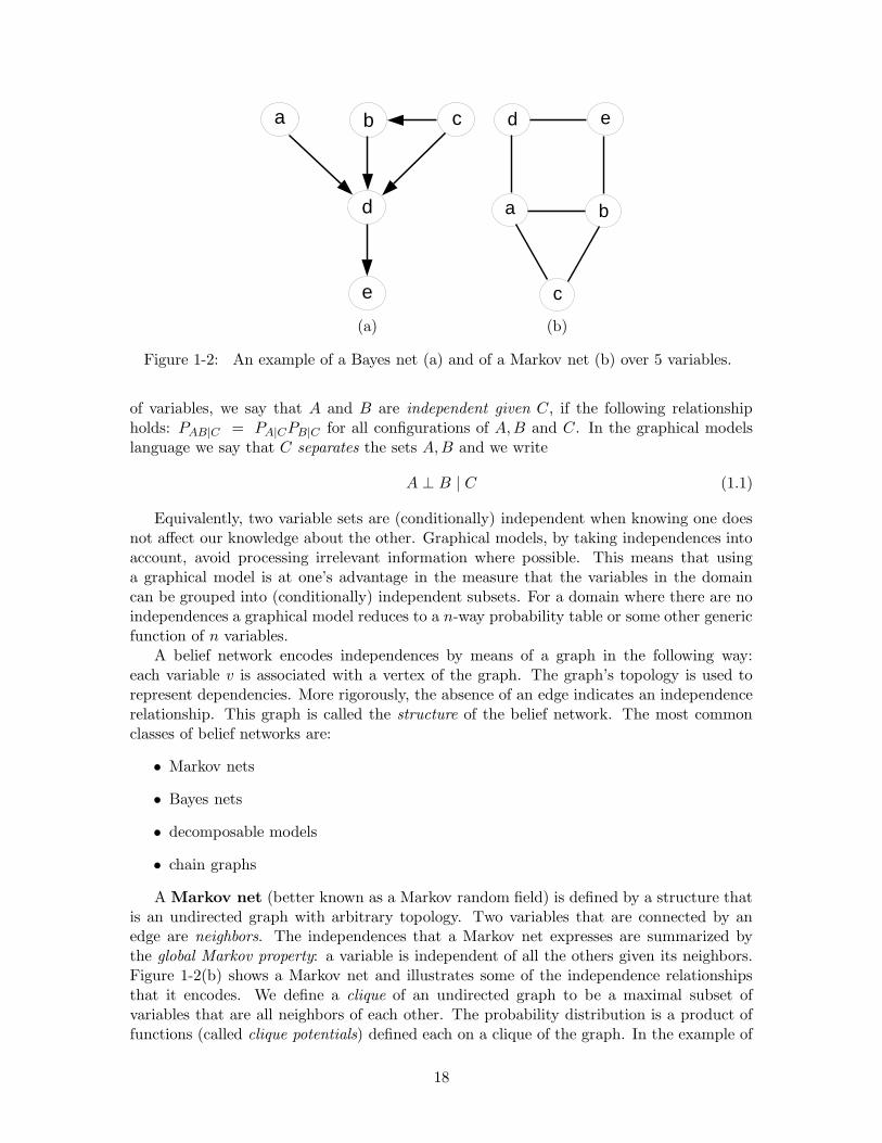
e

d

b ca ed

b

c

a

(a) (b)

Figure 1-2: An example of a Bayes net (a) and of a Markov net (b) over 5 variables.

of variables, we say that A and B are independent given C, if the following relationshipholds: PAB|C = PA|CPB|C for all configurations of A,B and C. In the graphical modelslanguage we say that C separates the sets A,B and we write

A ⊥ B | C (1.1)

Equivalently, two variable sets are (conditionally) independent when knowing one doesnot affect our knowledge about the other. Graphical models, by taking independences intoaccount, avoid processing irrelevant information where possible. This means that usinga graphical model is at one’s advantage in the measure that the variables in the domaincan be grouped into (conditionally) independent subsets. For a domain where there are noindependences a graphical model reduces to a n-way probability table or some other genericfunction of n variables.

A belief network encodes independences by means of a graph in the following way:each variable v is associated with a vertex of the graph. The graph’s topology is used torepresent dependencies. More rigorously, the absence of an edge indicates an independencerelationship. This graph is called the structure of the belief network. The most commonclasses of belief networks are:

• Markov nets

• Bayes nets

• decomposable models

• chain graphs

A Markov net (better known as a Markov random field) is defined by a structure thatis an undirected graph with arbitrary topology. Two variables that are connected by anedge are neighbors. The independences that a Markov net expresses are summarized bythe global Markov property: a variable is independent of all the others given its neighbors.Figure 1-2(b) shows a Markov net and illustrates some of the independence relationshipsthat it encodes. We define a clique of an undirected graph to be a maximal subset ofvariables that are all neighbors of each other. The probability distribution is a product offunctions (called clique potentials) defined each on a clique of the graph. In the example of

18

figure 1-2(b) the cliques are a, b, c, a, d, d, e, b, e; c ⊥ d, e | a, b; d ⊥ b | a, e; e ⊥ a | b, dare among the independences represented by this net.

Thus, the Markov net is specified in two stages: first, a graph describes the structure ofthe model. The structure implicitly defines the cliques. Second, the probability distributionis expressed as a product of functions of the variables in each clique and some parameters.We say that the distribution factors according to the graph. For example, a distributionthat factors according to the graph in figure 1-2 is represented by

P = φabcφadφdeφbe (1.2)

The number of variables in each clique is essential for the efficiency of the computationscarried by the model. The fewer variables in any clique, the more efficient the model. Thetotality of the parameters corresponding to the factor functions forms the parameter setassociated with the given graph structure.

Bayes nets are belief nets whose structure is a directed graph that has no directedcycles; such a structure is called a directed acyclic graph, or shortly a DAG. We denote by~uv an edge directed from u to v and in this case we call u the parent of v. A descendent of uis a variable w that can be reached by a directed path starting at u; hence, the children ofu, their children, and so on, are all descendents of u. Figure 1-2(a) depicts an example of aDAG. The independences encoded by a Bayes net are summarized by the directed Markovproperty, that states that in a Bayes net, any variable is independent of its non-descendentsgiven its parents. The probability distribution itself is given in a factorized form thatcorresponds to the independence relationships expressed by the graph. Each factor is afunction that depends on one variable and all its parents (we call this set of variables afamily). For example, in figure 1-2(a) the families are a, c, b, c, b, c, d, d, e. Thelist of independences encoded by this net includes a ⊥ b, a, b, c ⊥ e|d. Any distributionwith this structure can be represented as

P = PaPcPb|cPd|bcPe|d (1.3)

In short, for both classes of belief nets, the model is specified by first specifying itsstructure. The structure determines the subsets of “closely connected” variables (cliquesin one case, families in the other) on which we further define the factor functions (cliquepotentials or conditional probabilities) that represent the model’s parametrization.

Any probability distribution P that can be factored according to a graph G (DAG orundirected) and thus possesses all the independences encoded in it is called conformal to G.The graph G is called an I-map of P . If G is an I-map of P then only the independencesrepresented in G will be useful from the computational point of view even though a beliefnet with structure G will be able to represent P exactly. If the distribution P has no otherdependencies then those represented by G, G is said to be a perfect map for P . For anyDAG or undirected graph there is a probability distribution P for which G is a perfectgraph. The converse is not true: there are distributions whose set of independences doesnot have a perfect map.

Decomposable models. Bayes nets and Markov nets represent distinct but intersect-ing classes of distributions. A probability distribution that can be mapped perfectly asboth a Bayes net and a Markov net is called a decomposable model. In a decomposablemodel, the cliques of the undirected graph representation play a special role. They canbe arranged in a tree (i.e acyclic graph) structure called junction tree. The vertices of thejunction tree are the cliques. The intersection of two cliques that are neighbors in the tree

19

is always non-void and is called a separator. Any probability distribution that is factorizedaccording to a decomposable model can be refactorized according to the junction tree intoclique potentials φC and separator potentials φS in a way that is called consistent and thatensures the following important property:

The junction tree consistency property If a junction tree is consistent [38, 36] thenfor each clique C ⊂ V the marginal probability of C is equal to the clique potential φC .

The factorization itself has the form

P =

∏C φC∏S φS

(1.4)

From now on, any reference to a junction tree should implicitly assume that the treeis consistent. This property endows decomposable models with a certain computationalsimplicity that is exploited by several belief network algorithms. We will discuss inferencein junction trees in section 1.3.4.

Chain graphs [44] are a more general category of graphical models. Their underlyinggraph comprises both directed and undirected edges. Bayes nets and Markov nets are bothsubclasses of chain graphs.

1.3.2 Advantages of graphical models

The advantages of a model that is factorized according to the independences between vari-ables are of several categories:

• Flexibility and modeling power. The flexible dependence topology, complementedby the freedom in the choice of the factor functions, makes belief network a rich andpowerful class among probabilistic models. In particular, belief networks encompassand provide a unifying view of several other model classes (including some that areused for supervised learning): hidden Markov models, Boltzmann machines, stochasticneural networks, Helmholtz machines, decision trees, mixture models, naive-Bayesmodels.

More important perhaps than the flexibility of the topology is the flexibility in theusages that graphical models admit. Because a belief network represents a probabilitydistribution, any query that can be expressed as a function of probabilities over subsetsof variables is acceptable. This means that in particular, a belief network can be usedas a classifier for any variable of its domain, can be converted to take any two subsetsof variables as inputs and outputs respectively and to compute probabilities of theoutputs given the inputs or can be used for diagnostic purposes by computing themost likely configuration of a set of variables given another set.

This flexibility is theoretically a property of any probability density model, but not alldensity representations are endowed with the powerful inference machine that allowsone to compute arbitrary conditional probabilities and thus to take advantage of it.

• The models are easier to understand and to interpret. A wide body of practi-cal experience shows that graphical representations of dependencies are very appealingto the (non-technical) users of statistical models of data. Bayes nets, which allow forthe interpretation of a directed edge ~uv as a causal effect of u on v, are particularlyappreciated as a means of knowledge elicitation from human domain experts. More-over, in a Bayes net the parameters represent conditional probabilities; it is found that

20

specifying or operating with conditional probabilities is much easier for a human thanoperating with other representations (as for example, specifying a joint probability)[55].

The outputs of the model, being probabilities, have a clear meaning. If we give theseprobabilities the interpretation of degrees of belief, as advocated by [55], then a beliefnetwork is a tool for reasoning under uncertainty.

• Advantages in learning the parameters from data for a given structure.More independences mean fewer free parameters compared to a full probability model(i.e. a model with no independences) over the same set of variables. Each parameterappears in a function of only a subset of the variables, thus depends on fewer variables.Under certain parametrizations that are possible for any Bayes net or Markov netstructure, this allows for independent estimation of parameters in different factors.In general, for finite amounts of data, a smaller number of (independent) parametersimplies an increased accuracy in the estimation of each parameter and thus a lowermodel variance.

• Hidden variables and missing data. A hidden variable is a variable whose valueis never observed3. Other variables may on some occasions be observed, but not inothers. When the latter happens, we say that the current observation of the domainhas a missing value for that variable. If in an observation (or data point) no variableis missing, we say that the observation is complete. The graphical models frameworkallows variables to be specified as observed or unobserved for any data point, inte-grating thus supervised learning and naturally handling both missing data and hiddenvariables.

1.3.3 Structure learning in belief networks

Learning the structure of a graphical model from data, however, is not an easy task. [33]formulates the problem of structure learning in Bayes networks as a Bayesian model selectionproblem. They show that under reasonable assumptions the prior over the parameters ofa Bayes network over a discrete variable domain has the form of a Dirichlet distribution.Moreover, given a set of observations, the posterior probability of a network structure canbe computed in closed form. Similar results can be derived for continuous variable modelswith jointly Gaussian distributions [32]. However, finding the structure with the highestposterior probability is an intractable task. For general DAG structures, there are noknown algorithms for finding the optimal structure that are asymptotically more efficientthan exhaustive search.

Therefore, in the majority of the applications, the structure of the model is eitherassessed by a domain expert, or is learned by examining structures that are close to oneelicited from prior knowledge. If neither of these is the case, then usually some simplestructure is chosen.

3One can ask: why include in the model a variable that is never observed? One reason is that ourphysical model of the domain postulates the variable, although in the given conditions we cannot observe itdirectly (e.g. the state of a patients liver is only assessed indirectly, by certain blood-tests). Another reasonis of computational nature: we may introduce a hidden variable because the resulting model explains theobserved data well with fewer parameters than the models that do not include the hidden variable. Thisis often the case for hidden causes: for a second example from the medical domain, a disease is a hiddenvariable that allows one to describe in a simple way the interplay between a multitude of observation factscalled symptoms. In chapter 6 we discuss this issue at length.

21

1.3.4 Inference and decomposable models

The task of using a belief network in conjunction with actual data is termed inference.In particular, inference means answering a generic query to the model that has the form:Q=“what is the probability of variable v having value xv given that the values of thevariables in the subset V ′ ⊂ V are known?”. The variables in V ′ and their observed valuesare referred to as categorical evidence and denoted by E . In a more general setting, one candefine evidence to be a probability distribution over V ′ (called a likelihood) but this casewill not be considered here. Thus, inference in the restricted sense can be formally definedas computing the probability P (v = xv|E) in the current model. This query is importantfor two reasons: One, the answers to a wide range of common queries can be formulated asa function of one or more queries of type Q or can be obtained by modified versions of theinference algorithm that solves the query Q. Two, Q serves as a benchmark query for theefficiency of the inference algorithms for a given class of belief networks.

Inference in Bayes nets. In [55] Pearl introduced an algorithm that performs exactinference in singly connected Bayes networks, called by him polytrees. A singly connectedBayes net is a network whose underlying undirected graph has no cycles. In such a net therewill always be at most one (undirected) path between any two variables u and v. Pearl’salgorithm, as it came to be named, assumes that each node can receive/send messages onlyfrom/to its neighbors (i.e. its parents and children) and that it performs computationsbased only on the information locally present at each node. Thus it is a local algorithm.Pearl proves that it is also asynchronous, exact and that it terminates finite time. Theminimum running time is bounded above by the diameter of the (undirected) graph, whichin turn is less or equal to the number of variables n.

The singly-connectedness of the graph is essential for both the finite termination and thecorrectness of the algorithm’s output4. For general multiply connected Bayes nets, inferenceis provably NP-hard [8].

The standard way of performing inference in a Bayes net of general topology is totransform it into a decomposable model; this is always possible by a series of edge additionscombined with removing the edges’ directionality. Adding edges to a graphical model doesnot change the probability distribution that it represents but will “hide” (and thus makecomputationally unusable) some of its independences. Once the decomposable counterpartof the Bayes net is constructed, inference is performed via the standard inference algorithmfor decomposable models, the Junction Tree Algorithm that will be described below.

Inference in junction trees. As defined before, a decomposable model (or junc-tion tree) is a belief network whose cliques form a tree. Tree distributions, which will beintroduced in the next section, are examples of decomposable models.

Inference in a graphical model has 3 stages. Here these stages are described for thecase of the junction tree and they represent what is known as the Junction Tree algorithm[38, 36]:

Entering evidence. This step combines a joint distribution over the variables (whichcan be thought of as a prior) with evidence (acquired from a different source of in-formation) to produce a posterior distribution of the variables given the evidence.

4It is worth mentioning, however, that recently some impressively successful applications of Pearl’s algo-rithm to Bayes networks with loops have been published. Namely the Turbo codes [3], Gallager [26] andNeal-MacKay [46] codes that are all based on belief propagation in multiply connected networks. WhyPearl’s algorithm performs well in these cases is a topic of intense current research [70].

22

The expression of the posterior is in the same factorized form as the original distri-bution, but at this stage it does not satisfy all the consistency conditions implicit inthe graphical model’s (e.g. junction tree’s) definition.

Propagating evidence. This is a stage of processing whose final result is the pos-terior expressed as a consistent and normalized junction tree. Often this phase is re-ferred to as the Junction Tree algorithm proper. The Junction tree algorithm requiresonly local computations (involving only the variables within one clique). Similarly toPearl’s algorithm for polytrees, information is propagated along the edges of the tree,by means of the separators. The algorithm is exact and finite time; it requires a num-ber of basic clique operations proportional to the number of cliques in the tree. If allthe variables of the domain V take values in finite sets, the time required for the basicinference operations in a clique is proportional to the size of total state space of theclique (hence it is exponential in cardinality of the clique). The total time requiredfor inference in a junction tree is O( the sum of these state space sizes ).

Extracting the probabilities of the variables of interest by marginalization inthe joint posterior distribution obtained at the end of the previous stage. In a consis-tent junction tree the marginal of any variable v can be computed by marginalizationin any φC for which v ∈ C. If the clique sizes are small relative to n, this representsan important saving w.r.t. the time for computing the marginal. This is also thereason for the locality of the operations necessary in the previous step of the inferenceprocedure.

Returning to Bayes nets, it follows that the time required for inference by the junctiontree method is exponential in the size of the largest clique of the resulting junction tree. It ishence desirable to minimize this quantity (or alternatively the sum of the state space sizes)in the process of constructing the decomposable model. However, the former objective isprovably NP-hard (being equivalent to solving a max-clique problem) [2]. It is expected,but not yet known, that the alternative objective is also an NP-hard problem. Moreover,it has been shown by [37] that any exact inference algorithm based on local computationsis as least as hard as the junction tree algorithm and thus also NP-hard.

Inference in Markov nets. [30] showed that inference in Markov random fields witharbitrary topology is also intractable. They introduced a Markov chain Monte Carlo sam-pling technique for computing approximate values of marginal and conditional probabilitiesin such a network that is known as simulated annealing.

Similar approaches of approximate inference by Monte Carlo techniques have been de-vised and used for Bayes nets of small size also [31, 61].

Approximate inference in Bayes nets is a topic of current research. The existent ap-proaches include: pruning the model and performing exact inference on the reduced model[40], cutting loops and bounding the incurred error [19], variational methods to bound thenode probabilities in sigmoidal belief networks [35, 39].

1.4 Why, what and where? Goal, contributions and roadmap of the thesis

The previous sections have presented the challenge of density estimation for multidimen-sional domains and have introduced models as tools specifically designed for this purpose.

23

It has been shown that graphical models focus on expressing the dependencies betweenthe variables of the domain, without constraining neither the topology of these dependencies,nor their functional form. The property of separating the dependency structure from itsdetailed functional form makes them an excellent support for human intuition, whitoutcompromising the modeling power of this model class.

The probabilistic semantics of a graphical model makes it possible to separate modellearning from its usage: once a belief network is constructed from data, one can use it inany way that is consistent with the laws of probability.

We have seen also that inference in graphical models can be performed efficiently whenthe models are simple, but that in the general case it is an NP-hard problem. The sameholds for learning a belief network structure from data: learning is hard in general, but weshall see that there are classes of structures for which both learning the structure and theparameters can be done efficiently.

It is the purpose of this thesis to propose and to describe a class of models that is richenough to be useful in practical applications yet admits tractable inference and learningalgorithms. This class is the class of mixtures of trees.

1.4.1 Contributions

Mixture of trees models . A tree can be defined as a Bayes net in which each node hasat most one parent. But trees can represent only acyclic pairwise dependencies and thus havea limited modeling power. By combining tree distributions in a mixture, one can representany distribution over discrete variables. The number of trees (or mixture components) is aparameter controlling the model’s complexity. Mixtures of trees can represent a different setof dependencies than graphical models. From the algorithmic perspective, this thesis showsthat the properties of tree distributions, namely the ability to perform the basic operationsof computing likelihoods, marginalization and sampling in linear time, directly extend tomixtures.

An efficient learning algorithm. This thesis introduces an efficient algorithm for es-timating mixtures of trees from data. The algorithm builds upon a fundamental propertyof trees, the fact that unlike almost any other class of graphical models, a tree’s structureand parameters can be learned efficiently. Embedding the tree learning algorithm in anExpectation-Maximization search procedure produces an algorithm that is quadratic in thedomain dimension n and linear in the number of trees m and in the size of the data set N .The algorithm finds Maximum Likelihood estimates but can serve for Bayesian estimationas well. To preserve the algorithm’s efficiency in the latter case, one needs to use a restrictedclass of priors. The thesis characterizes this class as being the class of decomposable priorsand shows that the restrictions that this class imposes are not stronger than the assump-tions underlying the mixture of trees learning algorithm itself. It is also shown that manywidely used priors belong to this class.

An accelerated learning algorithm for sparse binary data. If one has in mind appli-cation over high-dimensional domains like document categorization and retrieval, preferencedata or image compression, a quadratic algorithm may not be sufficiently fast. Therefore, Iintroduce an algorithm that exploits a property of the data – sparsity – to construct a fam-ily of algorithms that are jointly subquadratic. In controlled experiments on artificial data

24

Introduction

Trees

Mixturesof Trees

Bayesian

Hiddenvariable

discovery

Experiments

Accelerated

Conclusion

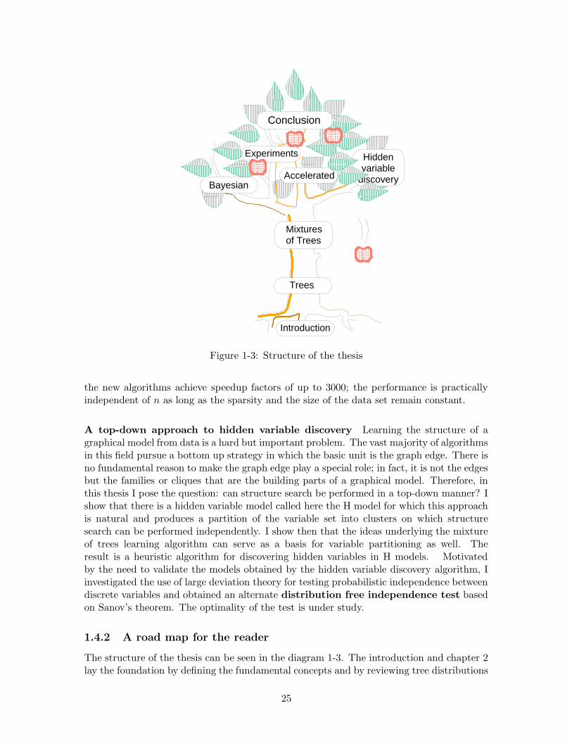
Figure 1-3: Structure of the thesis

the new algorithms achieve speedup factors of up to 3000; the performance is practicallyindependent of n as long as the sparsity and the size of the data set remain constant.

A top-down approach to hidden variable discovery Learning the structure of agraphical model from data is a hard but important problem. The vast majority of algorithmsin this field pursue a bottom up strategy in which the basic unit is the graph edge. There isno fundamental reason to make the graph edge play a special role; in fact, it is not the edgesbut the families or cliques that are the building parts of a graphical model. Therefore, inthis thesis I pose the question: can structure search be performed in a top-down manner? Ishow that there is a hidden variable model called here the H model for which this approachis natural and produces a partition of the variable set into clusters on which structuresearch can be performed independently. I show then that the ideas underlying the mixtureof trees learning algorithm can serve as a basis for variable partitioning as well. Theresult is a heuristic algorithm for discovering hidden variables in H models. Motivatedby the need to validate the models obtained by the hidden variable discovery algorithm, Iinvestigated the use of large deviation theory for testing probabilistic independence betweendiscrete variables and obtained an alternate distribution free independence test basedon Sanov’s theorem. The optimality of the test is under study.

1.4.2 A road map for the reader

The structure of the thesis can be seen in the diagram 1-3. The introduction and chapter 2lay the foundation by defining the fundamental concepts and by reviewing tree distributions

25

and their inference and learning algorithms.Chapter 3 builds on this to define the mixture of trees with its variants, to introduce the

algorithm for learning mixtures of trees from data in the Maximum Likelihood frameworkand to show that mixtures of trees can approximate arbitrarily closely any distribution overa discrete domain.

The following chapters will each develop this material into a different direction and thuscan be read independently in any order. Chapter 4 discusses learning mixtures of trees in aBayesian framework. The basic learning algorithm is extended to take into account a classof priors called decomposable priors. It is shown that this class is rich enough to containimportant priors like the Dirichlet prior and Minimum Description Length type priors. Inthis process, the assumptions behind decomposable priors and the learning algorithm itselfare made explicit and discussed.

Chapter 5 aims to improve the computational properties of the tree learning algorithm.It introduces a data representation and two new algorithms that exploit the properties ofthose domains to construct exact Maximum Likelihood trees in subquadratic time. Thecompatibility of the new algorithms with the EM framework and with the use of decom-posable priors are also discussed.

The next chapter, 6, introduces the top-down method for learning structures with a hid-den variable, methods for scoring the obtained models and a discussion of the independencetest approach to validating them.

Finally there comes the chapter devoted to experimental assessments. Chapter 7 demon-strates the performance of mixtures of trees on various tasks. There are very good resultsin density estimation, even for data that are not generated from a mixture of trees. Thelast part of this chapter discusses classification with mixtures of trees. Although the modelis a density estimator, its performance as a classifier in my experiments is excellent, even incompetition with classifiers trained in supervised mode. I analize the behavior of the singletree classifier and demonstrate that it acts like an implicit feature selector.

The last chapter, 8 contains the concluding remarks.

26

Chapter 2

Trees and their properties

I think that I shall never seeA poem as lovely as a tree.Joyce Kilmer–Trees

In this section we introduce tree distributions as a subclass of decomposable models andwe demonstrate some of the properties that make them attractive from a computationalpoint of view. It will be shown that fundamental operations on distributions: inference,sampling and marginalizing carry over directly from their junction tree counterparts andare order n or less when applied to trees. Learning tree distributions will be formulated asMaximum Likelihood (ML) estimation problem. To solve it, an algorithm will be presentedthat finds the tree distribution T that best approximates a given target distribution P inthe sense of the Kullback-Leibler divergence. The algorithm optimizes over both structureand parameters, in time and memory proportional to the size of the data set and quadraticin the number of variables n. Some final considerations on modeling power and ease ofvisualization will prepare the introduction of mixtures of trees in the next section.

2.1 Tree distributions

In this section we will introduce the tree model and the notation that will be used throughoutthe paper. Let V denote the set of variables of interest. As stated before, the cardinalityof V is |V | = n. For each variable v ∈ V let rv denote its number of values, Ω(v) representits domain and xv ∈ Ω(v) a particular value of v. Similarly, for subset A of V , Ω(A) =⊗v∈A Ω(v) is the domain of A and xA an assignment to the variables in A. In particular,

Ω(V ) is the state-space of all the variables in V ; to simplify notation xV will be denotedby x. Sometimes we shall need the maximum of rv over V ; we shall denote this value byrMAX .

According to the graphical model paradigm, each variable is viewed as a vertex of an(undirected) graph (V,E). An edge connecting variables u and v is denoted by (uv) andits significance will become clear in the following. The graph (V,E) is called a tree if it hasno cycles1. Note that under this definition, a tree can have a number p between 1 and |V |connected components. The number of edges |E| and p are in the relationship

|E|+ p = |V | (2.1)

1This definition differs slightly from the definition of a tree in the graph theory literature. There, a treeis required to have no cycles and to be connected (meaning that between every two vertices there shouldexist a path); our definition of a tree allows for disconnected graphs to be trees and corresponds to what ingraph theory is called a forest.

27

which means that adding an edge to a tree reduces the number of connected componentsby 1. Thus, a tree can have at most |V | − 1 = n− 1 edges.

Now we define a probability distribution T that is conformal with a tree. Let us denoteby Tuv and Tv the marginals of T for u, v ∈ V and (uv) ∈ E:

Tuv(xu, xv) =∑

x|u=xu,v=xv

T (x) (2.2)

Tv(xv) =∑

x|v=xvT (x). (2.3)

They must satisfy the consistency condition

Tv(xv) =∑

xu

T (xv, xu) ∀u, v, (uv) ∈ E (2.4)

Let deg v be the degree of vertex v, i.e. the number of edges incident to v ∈ V . Then, thedistribution T is conformal with the tree (V, E) if it can be factored as:

T (x) =

∏(u,v)∈E Tuv(xu, xv)∏v∈V Tv(xv)deg v−1

(2.5)

The distribution T itself will be called a tree when no confusion is possible. The graph(V,E) represents the structure of the distribution T . Noting that for all trees over the samedomain V the edge set E alone uniquely defines the tree structure, in the following whenno confusion is possible we identify E with the structure. If the tree is connected, i.e. itspans all the nodes in V , it is sometimes called a spanning tree.

Because a tree is a triangulated graph it is easy to see that a tree distribution is adecomposable model. In fact, the above representation (2.5) is identical to the junction treerepresentation of T . The cliques identify with the graph’s edges (hence all cliques are sizetwo) and the separators are all the nodes of degree larger than one. Thus the junction treeis identical to the tree itself with the clique and separator potentials being the marginalsTuv and Tv, deg v > 1 respectively.

This shows a remarkable property of tree distributions: a distribution T that is conformalwith the tree (V,E) is completely determined by its edge marginals Tuv, (uv) ∈ E.

Since every tree T is a decomposable model it can be represented in terms of conditionalprobabilities

T (x) =∏

v∈VTv|pa(v)(xv|xpa(v)) (2.6)

We shall call the representations (2.5) and (2.6) the undirected and directed tree represen-tations respectively. The form (2.6) is obtained from (2.5) by choosing an arbitrary rootin each connected component and directing each edge away from the root. In other words,if for (uv) in E, u is closer to the root than v, then u becomes the parent of v and isdenoted by pa(v). Note that in the directed tree thus obtained, each vertex has at mostone parent. Consequently, the families of a tree distribution are either of size one (theroot or roots) or of size two (the families of the other vertices). After having transformedthe structure into a directed tree one computes the conditional probabilities corresponding

to each directed edge by recursively substitutingTvpa(v)

Tpa(v)by Tv|pa(v) starting from the root.

pa(v) represents the parent of v in the thus directed tree or the empty set if v is the root

28

of a connected component. The directed tree representation has the advantage of havingindependent parameters. The total number of free parameters in either representation is

∑

(u,v)∈Erurv −

∑

v∈V(deg v − 1)rv − p =

=∑

(u,v)∈E(ru − 1)(rv − 1) +

∑

v∈Vrv − n (2.7)

The r.h.s. of (2.7) shows that each newly added edge (uv) increases the number ofparameters by (ru − 1)(rv − 1).

Now we shall characterize the set of independences represented by a tree. In a tree thereis at most one path between every two vertices. If node w is on the path between u andv we say that w separates u and v. Correspondingly, if we set w as a root, the probabilitydistribution T can be decomposed into the product of two factors, each one containing onlyone of the variables u, v. Hence, u and v are independent given w:

u ⊥ v | w

Therefore we conclude that in a tree two variables are separated by any set that intersectsthe path between them. Two subsets A,B ⊂ V are independent given C ⊂ V if C intersectsevery path between u ∈ A and v ∈ B.

We can also verify that for a tree the undirected Markov property holds. The set ofvariables connected by edges to a variable v, namely its neighbors separates v from all theother variables in V .

2.2 Inference, sampling and marginalization in a tree distri-bution

This section discusses the basic operations: inference, marginalization and sampling fortree distributions. It demonstrates that the algorithms for performing these operations aredirect adaptations of their counterparts for junction trees and are heavily relying on thegeneric Junction Tree algorithm. It is also shown that all basic operations are linear in thenumber of variables n. This fact is important because the analog operations on mixtures oftrees use the algorithms for trees as building blocks. The details of the algorithms however,although presented here for the sake of completeness, can be skipped without prejudice forthe understanding of the rest of the thesis.

2.2.1 Inference.

As shown already, tree distributions are decomposable models and the generic inferencealgorithm for trees is an instance of the inference algorithm for decomposable models calledthe Junction Tree algorithm. We shall define it as a procedure, PropagateEvidence(T, E)that takes as inputs a tree having structure (V,E) presented in the undirected factored rep-resentation and some categorical evidence E on a set A ⊂ V . The procedure performs thefirst two steps of the inference process as defined in section 1.3.4. It enters the categoricalevidence by multiplying the original distribution T with a 0, 1-values function represent-ing the categorical evidence. Then it calibrates the resulting tree by local propagation ofinformation between the cliques (edges) of the tree. Finally, it outputs the tree T ∗ that is

29

factored conformally to the original T and represents the posterior distribution TV |E . Thealgorithm is described in detail in the last section of this chapter. It is also demonstratedthat it takes a running time of the order O(r2

MAX |E|).The last step, extracting the probabilities of variables of interest from the above men-

tioned representation is done by marginalization and will be discussed in the next section.In particular, obtaining the posterior probability of any single variable involves marginal-ization over at most one other variable which takes O(rMAX) operations.

2.2.2 Marginalization

In a junction tree, computing the marginal distribution of any group of variables thatare contained in the same clique can be performed by marginalization within the respectiveclique. For a tree, whose cliques are size two, the marginal of each variable v can be obtainedeither directly as Tv (if v is a separator and separator potentials are stored explicitly) or bymarginalizing in the potential Tuv of the edge incident to v (if v is a leaf node). Thus, themarginal for any single variable can be obtained in O(rMAX) additions.

The pairwise marginals for all the variables that are neighbors in T are directly availableas the clique potentials Tuv. The above enumeration exhausts all the cases where themarginals are directly available from the tree distribution. In the following I describean algorithm that can efficiently compute the marginal distributions for arbitrary pairs ofvariables. The algorithm can be generalized to marginal distributions over arbitrary subsetsof V .

First, it will be shown that the marginal Tuv depends only on the potentials of the edgeson the path between u and v in E. Let path(u, v) = (w0 = u,w1, w2, . . . , wd = v) be thevertices on the path between u and v in the tree (V,E) and let d ≥ 1 be its length. Then,the marginal Tuv can be expressed as

Tuv =∑

xV \u,v

T

=∑

xV \u,v

Tu

d∏

i=1

Twi|wi−1

∏

w′∈V \path(u,v)

Tw′|pa(w′)

(2.8)

=∑

xV \u,v

Tu

d∏

i=1

Twi|wi−1 (2.9)

=∑

xwi ,i=1,d−1

∏di=1 Twi−1wi∏d−1i=1 Twi

(2.10)

The first form (2.8) is obtained as the directed tree representation with a root at u. Sum-mation over each xw′ not on the path from u to v can be done recursively starting from theleaves of the tree and results in a factor of 1. Thus the form (2.9) is obtained. The thirdform, (2.10) is the rewriting of the previous equation in the undirected representation.

Each of the intermediate variables wi appears in only two factors of (2.9); consequently,summation over the values of the intermediate variables can be done one variable at a time,

30

as indicated by the following telescoped sum:

Tvu =∑

xwd−1

Tv|wd−1 . . . Tw3|w2

∑

xw2

(Tu∑

xw1

Tw1|uTw2|w1)

︸ ︷︷ ︸Tw2u︸ ︷︷ ︸

Tw3u

(2.11)

The computation of one value of Tuv takes∑d−1i=1 rwi additions and multiplications; to com-

pute the whole marginal probability table we need to perform

rurv

d−1∑

i=1

rwi = O((d− 1)r3MAX)

operations.As the above equation shows, the intermediate sums involved in the computation of

Tuv are themselves marginal distributions. This suggests that if the intermediate sums arestored and if the pairs (uv) ∈/ E are enumerated in a judiciously chosen order, one cancompute all the pairwise marginal tables by summing over 1 variable only for each of them;in other words, all the pairwise marginals can be computed with O((n − 1)(n − 2)r3

MAX)operations.

Marginalization in the presence of evidence represents the third and last stepof inference, as presented in the previous subsection. This problem can be approached invarious ways, one of them being the polytree algorithm of [55]. The approach we present herefollows directly from the procedures for entering evidence, calibration and marginalizationintroduced above. To find T ∗uv = Tuv|EA for u, v ∈ V, A ⊂ V one has to

1. enter and propagate evidence by T ∗ ← PropagateEvidence(T, EA)2. compute the marginal T ∗uv

2.2.3 Sampling

Sampling in a tree is best performed using the directed tree representation. The value ofthe root node(s) is sampled from its (their) marginal distribution. Then, the value of eachof the other nodes is sampled from the conditional distribution given its parent P (v|pa(v)),recursively, starting from the root(s). This simple algorithm is the specialization of thealgorithm presented in [14] for sampling from a junction tree. In [12] an algorithm ispresented for sampling without replacement in a junction tree that can be immediatelyspecialized for trees.

Sampling in a tree in the presence of evidence is done, just like marginalization in thepresence of evidence, in two steps. First, one incorporates the evidence by the Propaga-teEvidence algorithm; second, sampling by the procedure described above is performedon the resulting conditional distribution.

2.3 Learning trees in the Maximum Likelihood framework

2.3.1 Problem formulation

First, I shall formulate the learning problem as a Maximum Likelihood (ML) estimationtask.

31

Assume a domain V and a set of observations from V called a dataset D = x1, x2, . . . xN.We further assume that these data were generated by sampling independently from an un-known tree distribution T 0 over V . The learning problem consists in finding the generativemodel T 0. According to the Maximum Likelihood principle the estimate of T 0 from D is themodel that maximizes the probability (or likelihood) of the observed data. Equivalently,one can search to optimize the logarithm of the likelihood, called log-likelihood, which leadsus to formulate the ML Learning Problem for trees as follows:

Given a domain V and a set of complete observations D, find a tree distribution T ∗ forwhich

T ∗ = argmaxT

∑

x∈Dlog T (x). (2.12)

2.3.2 Fitting a tree to a distribution

The solution to the ML Learning Problem has been published in [7] in the broader contextof finding the tree that best fits a given distribution P over the dataset D. The goodnessof fit is evaluated by the Kullback-Leibler (KL) divergence [43] between P and T :

KL(P ||T ) =∑

x∈DP (x) log

P (x)

T (x)(2.13)

Since the Chow and Liu algorithm will constitute a building block for the algorithms thatwill be developed in my thesis, I shall present it and its derivation here. The impatientreader can skip to the next subsection.

Let us start by examining (2.13). It is known [11] that for any two distributions P andQ, KL(P ||Q) ≥ 0 and that equality is attained only for Q ≡ P . The KL divergence can berewritten as

KL(P ||Q) =∑

x

P (x)[log P (x)− logQ(x)]

=∑

x

P (x) log P (x)−∑

x

P (x) logQ(x) (2.14)

Notice that the first term above does not depend onQ. Hence, minimizing the KL divergencew.r.t. Q is equivalent to maximizing the second term of (2.14) (called the cross-entropybetween P and Q) and we know that this is achieved for Q = P .

Now, let us return to our problem of fitting a tree to a fixed distribution P . Findinga tree distribution requires finding its structure (represented by the edge set E) and thecorresponding parameters, i.e. the values of Tuv(xu, xv) for all edges (uv) ∈ E and for allvalues xu, xv.

Assume first that the structure E is fixed and expand the right-hand side of (2.13):

KL(P ||T ) = (2.15)

=∑

x∈DP (x)[log P (x)− log T (x)]

= −∑

x∈DP (x) log

1

P (x)−∑

x∈DP (x) log[

∏

v∈VTv|pa(v)(xv|xpa(v))]

= −H(P )−∑

v∈V

∑

x∈DP (x) log Tv|pa(v)(xv|xpa(v))

32

= −H(P )−∑

v∈V

∑

xv ,xpa(v)

Pv,pa(v)(xv, xpa(v)) log Tv|pa(v)(xv |xpa(v))

= −H(P )−∑

v∈V

∑

xpa(v)

Ppa(v)(xpa(v))∑

xv

Pv|pa(v)(xv|xpa(v)) log Tv|pa(v)(xv|xpa(v))

In the above, H(P ) denotes the entropy of the distribution P , a quantity that does notdepend on T , and Puv, Pv represent respectively the marginals of u, v, v under P . Theinner sums in the last two lines are taken over the domains of v and pa(v) respectively.When v is a root node, pa(v) is the void set and its corresponding range has, by convention,one value with a probability of Ppa(v)(xpa(v)) = 1. Moreover, note that the terms thatdepend on T are of the form

−∑

xv

Pv|pa(v)(xv|xpa(v)) log Tv|pa(v)(xv|xpa(v))

which differs only by a constant independent of T from the KL divergence

KL(Pv|pa(v) ||Tv|pa(v))

We know that the latter is minimized by

Tv|pa(v)(. |xpa(v)) ≡ Pv|pa(v)(. |xpa(v)) ∀v ∈ V. (2.16)

Hence, for a fixed structure E, the best tree parameters in the sense of the minimum KLdivergence are obtained by copying the corresponding values from the conditional distribu-tions Pv|pa(v). Let us make two remarks: first, the identity (2.16) can be achieved for all vand xpa(v) because the distributions Tv|pa(v)=xpa(v)

are each parameterized by its own set of

parameters. Second, from the identity (2.16) it follows that

Tuv ≡ Puv ∀(u, v) ∈ E (2.17)

and subsequently, that the resulting distribution T is the same independently of the choiceof the roots. For each structure E we denote by TE the tree with edge set E and whoseparameters satisfy equation (2.17). TE achieves the optimum of (2.13) over all tree distri-butions conformal with (V,E).

Now, with the previous results in mind, we shall proceed to the minimization ofKL(P ||T )over the tree structures. First, notice that this task is equivalent to maximizing the objective

J(E) =∑

x∈DP (x) log TE(x). (2.18)

over all structures E.Expanding the above formula and using (2.17) we obtain successively:

J(E) = (2.19)

=N∑

i=1

P (xi) log TE(xi)

=N∑

i=1

P (xi)[∑

(u,v)∈Elog TEuv(x

iux

iv)−

∑

v∈V(deg v − 1) log TEv (xiv)] (2.20)

33

=N∑

i=1

P (xi)[∑

(u,v)∈ElogPuv(x

iux

iv)−

∑

v∈V(deg v − 1) log Pv(x

iv)] (2.21)

=∑

(u,v)∈E

N∑

i=1

P (xi)[ log Puv(xiux

iv)− log Pu(xiu)− logPv(x

iv)]

+∑

v∈V

N∑

i=1

P (xi) log Pv(xiv) (2.22)

=∑

(u,v)∈E

N∑

i=1

P (xi) logPuv(x

iux

iv)

Pu(xiu)Pv(xiv)+∑

v∈V

N∑

i=1

P (xi) log Pv(xiv) (2.23)

=∑

(u,v)∈E

∑

xuxv

Puv(xu, xv) logPuv(xu, xv)

Pu(xu)Pv(xv)+∑

v∈V

∑

xv

Pv(xv) log Pv(xv) (2.24)

=∑

(u,v)∈EIuv −

∑

v∈VH(Pv) (2.25)

Equation (2.20) follows from the undirected tree representation (2.5) of T E , (2.21) isobtained from (2.20) by taking into account (2.17); equation (2.23) follows from (2.22) byperforming a summation over all x ∈ D that have the same xu, xv and using the definitionsof Puv and Pv; finally in equation (2.24) the terms Iuv under the first sum sign representthe mutual information between the variables u and v under the distribution P :

Iuv =∑

xuxv

Puv(xu, xv) logPuv(xu, xv)

Pu(xu)Pv(xv)(2.26)

The mutual information between two variables is a quantity that is always non-negativeand equals 0 only when the variables are independent.

Remark two important facts about equation (2.25): first, the second sum does notdepend on the structure E; second and more importantly, the dependence of J(E) fromE is additive w.r.t. to the elements of the set E. In other words, each edge in (u, v) ∈ Econtributes a certain positive amount to J(E) and this amount Iuv is always the same,independently of the presence or absence of other edges and of the size of their contributions!

In this situation, maximization of J over all structures can be performed efficiently via aMaximum Weight Spanning Tree (MWST) algorithm [10] with weights Wuv = Iuv, u, v ∈V .

The MWST problem is formulated as follows: given a graph (V,E) and a set of realnumbers, called weights each corresponding to an edge of the graph, find a tree (V,E), E ∈ Efor which the sum of the weights corresponding to its edges is maximized. This problemcan be solved by a greedy algorithm that constructs the tree by adding one edge at a time,in decreasing order of the weights Wuv. There are several variants of the algorithm:the simplest one, called Kruskal’s algorithm, runs in O(n2 log n) time. Note that if all theweights are strictly positive, a tree with the maximum number of edges and p = 1 connectedcomponents will result. If some of the weights Wuv are zero, it is possible to obtain treeswith more than one connected component. More sophisticated MWST algorithms exist (seefor example [10, 65, 25, 20, 60]) and they improve on Kruskal’s algorithm on both runningtime and memory requirements. However, the running time of all published algorithms is atleast proportional to the number of candidate edges (|E|). In our case, this number is equalto n(n − 1)/2 since all pairs of variables have to be considered. Hence, the best running

34

time achievable for a MWST algorithm will be O(n2). Henceforth, we will assume that theMWST algorithm runs in O(n2) time and will not further specify the implementation.

All of the above are summarized in the TreeLearn algorithm

Algorithm TreeLearnInput Probability distribution P over domain V

Procedure MWST( weights ) that fits a maximum weight spanning tree over V .1. Compute marginals Pv, Puv for u, v ∈ V .2. Compute mutual informations Iuv for u, v ∈ V .3. Call MWST( Iuv ) that outputs the edge set E of a tree distribution T .4. Set Tuv ≡ Puv for (uv) ∈ E.Output T

The algorithm takes as input a probability distribution P over a domain V and outputsa tree distribution T that minimizes the KL divergence KL(P ||T ).

The running times for the algorithm’s steps are as follows:

steps 1,2. For steps 1. and 2. (computing the marginals and the mutual informations for all pairsof variables) the running time is dependent on the representation of P . But, generally,it should be expected to beO(n2), since there are n(n−1)/2 mutual information valuesto be computed.

step 3. The MWST algorithm takes O(n2) operations (or O(n2 log n) in Kruskal’s variant).

step 4. This step comprises only O(nr2MAX) assignments (remember that |E| < n).

Hence, the total running time of TreeLearn is O(n2 + nr2MAX) or O(n2) if we consider

rMAX to be a constant.

2.3.3 Solving the ML learning problem

The previous subsection has presented the algorithm TreeLearn(P ) that finds the treedistribution T ∗ closest in KL divergence to a given distribution P ,

T ∗ = argminT

KL(P ||T ).

To solve the initial Maximum Likelihood estimation problem it is sufficient to callTreelearn(P ) where P is the uniform distribution over the data

P (x) =

1N , x ∈ D0 otherwise

(2.27)

To see this, note that

KL(P ||T ) = − 1

N

N∑

i=1

log T (xi)− logN. (2.28)

Hence, minimizing the above expression is equivalent to maximizing the r.h.s. of equation(2.12).

For this case, the first step of the TreeLearn algorithm, computing the marginals, takesO(Nn2r2

MAX) time. This time dominates the times required for each of the following steps(unless Nr2

MAX < log n, which is usually not the case) and thus, the running time of theML tree estimation algorithm is O(Nn2r2

MAX).

35

2.4 Representation capabilities

If graphical representations are easy to grasp by means of human intuition, then the subclassof tree graphical models will be even more intuitive. For once, they are sparse graphs, havingn − 1 or fewer edges. More importantly and more precisely, between each two variablesthere is at most one path, or, in other words, the separation relationships between subsetsof variables, which are not easy to read out in a general Bayes net topology, are obviousin a tree. Thus, in a tree, an edge corresponds to the simplest common sense notion ofdirect dependency and is the natural representation for it. However, the very simplicitythat makes tree models intuitively appealing also limits their modeling power. In otherwords, the class of dependency structures representable by trees is a relatively small one.For instance, over a domain of dimension n there are nn−2 distinct (undirected) spanningtrees [71], but a total of 2n(n−1)/2 undirected graphs2. Mixture of trees models, whichwill be presented next, are a way of circumventing this problem. This thesis will showthat mixtures of trees can arbitrarily increase the representation power of tree distributionswhile sacrificing only little of their computational advantages and, to a certain extent, evenpreserving their appeal to human intuition.

2.5 Appendix: The Junction Tree algorithm for trees

This section will present the mechanisms for entering evidence in a tree density model andfor maintaining consistent representations in the presence of evidence.

Since a tree distribution is also a junction tree, inference will be done via the JunctionTree algorithm using the undirected tree representation (2.5) described previously.

Entering evidence In the general sense, evidence on a subset A of variables is definedto be a (possibly unnormalized) probability distribution

EA : Ω(A)→ [0,∞). (2.29)

A finding is a special type of evidence: A = v for some v ∈ V and fv ≡ Ev takes valuesin the set 0, 1 only. A finding on v represents a statement that v cannot take certainvalues. Any finding fv can be expressed as a sum of δ functions3 with as many non-zeroterms as the number of non-zero values of fv.

fv(xv) =∑

xv∈Ωv

fv(xv)δxv ,xv (2.30)

If EA consists of a collection of findings, one for each variable v ∈ A, such that:

EA =∏

v∈Afv (2.31)

the evidence is said to be categorical. Here and in the rest of the thesis, only categoricalevidence will be considered. For handling non-categorical evidence that is contained in oneclique, the reader is referred to [38]. [55] discusses another special case of non-categoricalevidence that is compatible with the polytree algorithm.

2To see that α = nn−2 < β = 2n(n−1)/2 note that α grows like nn while β grows like (2n/2)n andthat n < 2n/2 for n > 2.

3Dirac’s symbol δx,x is 1 if x = x and 0 otherwise

36

For any prior distribution PV of the variables in V and for any categorical evidence EA =δxA , A ⊂ V ,

P ∗V (xV \A, xA) = PV (xV \A, xA)EA(xA) (2.32)

represents the probability of xV \A, xA after observing the evidence EA. This probability isof course 0 for v 6= xv. Moreover, the conditional probability of the remaining variablesgiven the evidence is proportional to the above product

P ∗V \A|EA(xV \A) ∝ PV (x).EA(xA) (2.33)

Using the convention P ∗(xA|EA) = EA(xA) we express the posterior conditional distribu-tion of all the variables given the evidence EA as

P ∗V |EA(x) ∝ PV (x).EA(xA). (2.34)

The above equations and discussion easily generalizes to the case where EA is a productof sums of δ functions, i.e. the case of categorical evidence. Hence, for any categoricalevidence EA we define the operation of entering evidence by equation (2.34).

The normalization constant in equation (2.34) is

∑

x

P ∗V (x) (2.35)

which represents the prior probability of the categorical evidence P (EA) [38, 36]. Hence,the conditional probability of V given the (categorical) evidence EA is given by:

P ∗V |EA(x) =PV (x)EA(xA)

P (EA)(2.36)

For a tree distribution T , equation (2.34) rewrites as

T ∗V |EA(x) ∝ TV (x)EA(xA) (2.37)

and the prior of EA, given by (2.35) with P replaced by T , can be efficiently computed asit will be shown later.

Note also that because the posterior probability obtained by (2.34) is unnormalized, theevidence can be an unnormalized function as well.

Propagating evidence. When (categorical) evidence is entered in a tree T (or in adecomposable model), the resulting distribution T ∗V \A|EA is factored according to the graph

of T , but its factors (i.e. the clique potentials) are neither consistent (as a junction tree)nor normalized. The following step, called tree calibration has the purpose to make T ∗ anormalized and consistent distribution again. The calibration represents the Junction Treealgorithm proper and is applicable in general to any decomposable model, but what willbe presented here is its specialization for tree distributions. For the general case and theproofs of consistency, see [36] or [38].

It is important to keep in mind that calibration does not add any information to themodel, but merely reorganizes the information already present in order to represent it in aform that is convenient for subsequent use (e.g. marginalizations).

The basic operation in evidence propagation is called absorption. We say that edge (vw)absorbs from neighboring edge (uv) when the following procedure is called:

37

Algorithm Absorb

Absorb(u, v, w)Input edge potentials T ∗uv, Tvw, (uv), (vw) ∈ E1. T ∗v =

∑xu T

∗uv

2. Tv =∑xu Tuv

3. T ∗vw ← TvwT ∗vTv

Output T ∗vw

Note that absorption is an asymmetric operation: Absorb(u, v, w) and Absorb(w, v, u)produce different results. After an absorption, the potentials T ∗vw and T ∗uv are consistent. IfT ∗uv is normalized, so will be T ∗vw. If the potentials are already consistent, then an absorboperation in either direction changes nothing. These facts can be easily proved:

∑

xw

T ∗vw(xv, xw) =∑

xw

Tvw(xv, xw)T ∗v (xv)

Tv(xv)

=T ∗v (xv)

Tv(xv)

∑

xw

Tvw(xv, xw)

=T ∗v (xv)

Tv(xv)Tv(xv)

= T ∗v (xv)

=∑

xu

T ∗uv(xu, xv)

The above derivation proves consistency after absorption. Moreover, if the potentials areconsistent before absorption, then the fraction T ∗v (xv)

Tv(xv) equals 1 for all xv and absorption ineither direction leaves the potentials unchanged. Assume now that T ∗uv is normalized. Then

∑

xv ,xw

T ∗vw(xv, xw) =∑

xv

∑

xw

T ∗vw(xv, xw)

=∑

xv

T ∗v (xv)

=∑

xv

∑

xu

T ∗uv(xu, xv)

= 1

In the following it will be necessary to use absorption from multiple edges. This is definedas:

Algorithm Absorb

Absorb(u1, . . . , um, v, w)Input edge potentials T ∗uiv, Tvw, (uiv), (vw) ∈ E, i = 1, . . . m1. for i = 1, . . . ,m

T iv =∑xui

T ∗uiv2. Tv =

∑xu Tuv

3. Tvw ← Tvw∏mi=1

T ivTv

Output Tvw

We say that edge (vw) absorbs from adjacent edges (u1v), . . . (umv). Unlike the previouscase, after absorption from multiple edges, the potentials involved in the operation are not

38

necessarily consistent. To make them consistent, it would be sufficient for each of the edges(uiv) to absorb from (vw). As we shall see shortly, this is the idea behind the JunctionTree propagation algorithm: the whole tree is made consistent by a series of absorptionsfrom the periphery towards a “root edge” (or root clique) followed by a second series ofabsorptions in the opposite direction. The mechanism is implemented by two recursiveprocedures, CollectEvidence and DistributeEvidence which are described below.

When CollectEvidence from w is called for edge (v, w) ∈ E, then the edge callsCollectEvidence from v for all the other edges adjacent to v and then absorbs from them.

Algorithm CollectEvidenceCollectEvidence(T, v, w)

Input factored representation of tree Tnodes v, w, (vw) ∈ Elet n(v) = w, u1, . . . um, m ≥ 0

1. for i = 1, . . . ,mCollectEvidence(T, ui, v)

2. Absorb(u1, . . . um, v, w)Output T

CollectEvidence(v, w) fulfills the task of recursively absorbing from the subtree rootedin node v of edge (vw). DistributeEvidence(w, v) has the reverse effect: when it is calledfrom w for edge (vw) ∈ E, all the other edges adjacent to v absorb from (vw) then callDistributeEvidence from v.

Algorithm DistributeEvidenceDistributeEvidence(T,w, v)

Input factored representation of tree Tnodes v, w, (vw) ∈ Elet n(v) = w, u1, . . . um, m ≥ 0

1. for i = 1, . . . ,m1.1. Absorb(w, v, ui)1.2. DistributeEvidence(T, v, ui)

Output T

With the procedures above, we can introduce the Junction Tree algorithm, whose spe-cialization for trees (junction trees of cliquesize two) is called here PropagateEvidence.The algorithm takes as input a tree distribution T over the space Ω(V ) represented asa set of consistent, normalized marginal distributions Tuv, and some categorical evidenceEA, A ⊂ V . It outputs the distribution T ∗V |EA represented as a consistent, normalized treedistribution with the same structure as T . In this distribution, the marginals correspondingto the variables in A (the “observed” variables) will be δ functions.

39

Algorithm PropagateEvidencePropagateEvidence(T, EA)

Input a tree distribution T in factored representation conformal to (V,E)categorical evidence EA on a subset A ⊂ V

1. enter evidence: T ∗ ← TEA2. choose an edge (vw) ∈ E as root edge3. CollectEvidence(T ∗, w, v)

CollectEvidence(T ∗, v, w)

4. normalize: Z =∑xvxw T

∗vw T ∗vw ←

T ∗vwZ

5. DistributeEvidence(T ∗, w, v)DistributeEvidence(T ∗, v, w)

Output T ∗

The proofs of correctness for this algorithm are given in [38, 36]. The normalizationconstant Z computed in step 4 of the algorithm represents the probability of the evidenceT (EA). To see this, notice that the potential T ∗vw of the root edge does not change afterthe normalization. Moreover, all the other tree edges absorb, directly or indirectly, from(vw). Therefore, at the end of the algorithm, all the edge potentials will be normalized.Since the tree is consistent, by simple function identification we conclude that indeed eachT ∗v′w′, (v′w′) ∈ E represents the

The propagation of evidence in a tree distribution takes order O(r2MAX |E|) time.

40

Chapter 3

Mixtures of trees

The previous section has shown that in the framework of graphical probability models, treedistributions enjoy many properties that make them attractive as modeling tools: they havea flexible topology, are intuitively appealing, sampling and computing likelihoods are lineartime, simple efficient algorithms for marginalizing and conditioning (O(n2) or less) exist.Fitting the best tree to a given distribution can also be done exactly and efficiently. Treescan capture simple pairwise interactions between variables but they can prove insufficient formore complex distributions. Therefore, this chapter introduces a more powerful model, themixture of trees. As this thesis will show, mixtures of trees enjoy most of the computationaladvantages of trees and, in addition, they are universal approximators over the space of alldistributions.

We define a mixture of trees to be a distribution of the form

Q(x) =m∑

k=1

λkTk(x) (3.1)

with

λk ≥ 0, k = 1, . . . ,m;m∑

k=1

λk = 1. (3.2)

The tree distributions T k are the mixture components and λk are called mixture co-efficients. From the graphical models perspective, a mixture of trees can be viewed as acontaining an unobserved choice variable z, which takes value k ∈ 1, . . . m with probabil-ity λk. Conditioned on the value of z the distribution of the visible variables V is a tree.The m trees may have different structures and different parameters.

Note that because of the variable structure of the component trees, a mixture of treesis neither a Bayesian network nor a Markov random field. Let us adopt the notation

A ⊥P B | C (3.3)

for “A independent B given C under distribution P”. If for some (all) k ∈ 1, . . . m wehave

A ⊥T k B | C with A,B,C ⊂ Vthis will not imply that

A ⊥Q B | C.On the other hand, a mixture of trees is capable of representing dependency structures

that are conditioned on the value of one variable (the choice variable), something thata usual Bayesian network or Markov net cannot do. Situations where such a model ispotentially useful abound in real life: Consider for example bitmaps of handwritten digits.

41

ed

ca

ed

b

ca

ed

b

ca

z=1 z=2

z

z=3

b

Figure 3-1: A mixture of trees with m = 3 and n = 5. Note that although b ⊥T k c | a forall k = 1, 2, 3 this does not imply in general b ⊥ c | a for the mixture.

1

2

3 4 5

z

Figure 3-2: A Mixture of trees with shared structure represented as a graphical model.

42

They obviously contain many dependencies between pixels; however, the pattern of thesedependencies will vary across digits. Imagine a medical database recording the body weightand other data for each patient. The body weight could be a function of age and heightfor a healthy person, but it would depend on other conditions if the patient suffered froma disease or were an athlete. If, in a situation like the ones mentioned above, conditioningon one variable produces a dependency structure characterized by sparse, acyclic pairwisedependencies, then a mixture of trees will be the model most able to uncover and exploitthis kind of dependencies.

If we impose that all the trees in the mixture have the same structure we obtain amixture of trees with shared structure (MTSS). Note that even in this case the resultingmixture does not preserve the independence relationships of the component trees. But aMTSS can be represented as a Bayes net (after choosing an orientation for the trees) or,more directly, as a chain graph. Chain graphs were introduced by [45]; they represent asuperclass of both Bayes nets and Markov random fields [44]. A chain graph contains bothdirected and undirected edges. The representation of the MTSS as a graphical model isgiven in figure 3-2.

A simple modification of both the mixture of trees and the mixture of trees with sharedstructure is to have the choice variable be observed as well. Such models will be calledmixtures with visible choice variable in the forthcoming. Unless otherwise stated, it will beassumed that the choice variable is hidden. Therefore, sometimes it will be referred to ashidden variable.

3.1 Representation power of mixtures of trees

Here it will be shown that for discrete variable domains the class of mixtures of trees canrepresent any distribution.

Theorem Let V = v1, v2, . . . vn a set of variables with finite ranges and P a proba-bility distribution over Ω(V ). Then P can be represented as a mixture of trees.

Proof. Let us denote by δx∗ the distribution over Ω(V ) defined by

δx∗(x) =

1, x = x∗

0, otherwise(3.4)

δx∗ can be identified with a tree T x∗

having n connected components (i.e. a factoreddistribution) and

T x∗

vj =

1, vj = x∗j0, otherwise

for j = 1, . . . n. (3.5)

Moreover, any distribution P can be represented as a mixture of δ distributions:

P (x) =∑

x∗P (x∗)δx∗(x). (3.6)

where the sum is taken over the range of V and P (x∗) represent the mixing coefficients.This completes the proof.

43

3.2 Basic operations with mixtures of trees

Marginalization The marginal distribution of variables subset A ⊂ V is

QA(xA) =∑

xV \A

Q(x)

=∑

xV \A

m∑

k=1

λkTk(x)

=m∑

k=1

λk∑

xV \A

T k(x)

=m∑

k=1

λkTkA(xA) (3.7)

Hence, the marginal of Q is a mixture of the marginals of the component trees.

Inference (in the restricted sense) which is marginalization after conditioning on theevidence is performed in an analog way. Let EB be the evidence and B ⊂ V be the set ofvariables that the evidence is about. Then

QA(xA|EB) =∑

xV \(A∪B)

Q(x|EB) (3.8)

=m∑

k=1

λkTkA(xA|EB). (3.9)

One can also infer the value of the hidden variable given some evidence EB by applyingBayes’ rule

Pr[z = k|EB ] =Pr[EB|z = k]Pr[z = k]∑k′ Pr[EB|z = k′]Pr[z = k′]

(3.10)

=λkT

kB(EB)∑

k′ λk′Tk′B (EB)

(3.11)

In particular, when the evidence consists of observing all the visible variables E = v1 =x1, v2 = x2, . . . vn = xn, B = V and (x1, x2, . . . xn) = x the posterior probability distri-bution of z is

Pr[z = k|E ] ≡ Pr[z = k|x] =λkT

k(x)∑k′ λk′T

k′(x)(3.12)

Sampling Sampling in a mixture of trees, in the presence of evidence or not, is a straight-forward extension of sampling from one tree discussed in chapter 2.2. The procedure forsampling from a mixture of trees uses TreeSample( T, E) the procedure that samplesfrom a tree distribution given evidence E (possibly void)

Algorithm MixTreeSample( Q, E )Input a mixture of trees Q

evidence E1. sample k the value of z from (λ1, λ2, . . . λn)2. sample x from T k component of the mixture and returns a value x.

Output x

44

Conclusions As this subsection has shown, the basic operations on mixtures of trees,marginalization, conditioning and sampling, are direct extensions of the corresponding op-erations on tree distributions. Their complexity scales accordingly: Marginalization overa subset V \ A in a mixture of trees takes m times the computation for marginalizationover the same subset in a single tree. For instance, computing the marginal of a singlevariable (that is not in a separator) takes O(mr2

MAX). Inference in a mixture of trees takesm junction tree propagation operations, O(mnr2

MAX). Inferring the value of the hiddenvariable takes mn multiplications. Sampling from a mixture is O(m + n.ns), where ns isthe number of operations required to sample a value of a vertex in a clique, conditioned onthe value of the other vertex. For the directed tree representation ns ≤ rMAX . The choiceof the tree to sample from is an m-way choice requiring O(m) operations.

3.3 Learning mixtures of trees in the ML framework

3.3.1 The basic algorithm

This section will show how a mixture of trees can be fit to an observed dataset in theMaximum Likelihood paradigm via the EM algorithm [18].

The learning problem is similar to the one formulated for trees in chapter 2. We aregiven a set of observations D = x1, x2, . . . , xN and we are required to find the mixtureof trees Q that satisfies

Q = argmaxQ′

N∑

i=1

logQ(xi). (3.13)

Here and in the rest of the thesis we will assume that there are no missing values for thevariables in V . As for z we will first assume that it is hidden. We denote the (hidden)values of the choice variable by zi, i = 1, . . . N.

Learning the ML mixture of trees model will be done by means of the Expectation-Maximization (EM) algorithm. This is an iterative algorithm devised for fitting maximumlikelihood parameters for models with hidden or missing variables. Each iteration consistsof two steps, Expectation and Maximization, that will be described below.

The EM algorithm introduces a likelihood function called the complete log-likelihoodwhich is the log-likelihood of both the observed and the unobserved data given the currentmodel estimate M = m, T k, λk, k = 1, . . . m

lc(x1,...N , z1,...N |M) =

N∑

i=1

m∑

k=1

δk,zi(log λk + log T k(xi)) (3.14)

The complete log-likelihood depends on the unknown values of the hidden variable andtherefore it is not directly computable. The idea underlying the EM algorithm is to insteadcompute and optimize the expected value of lc.

The Expectation (E) step consists of estimating the posterior probability of the hiddenvariable for each of the observations. In our case this means estimating the probability ofeach tree generating data point xi

Pr[zi = k|xi,M] = γk(i) =λkT

k(xi)∑k′ λk′T

k′(xi)= E[δk,zi ] (3.15)

45

One uses these posterior probabilities to compute the expectation of lc, which is a linearfunction of the γk(i) values.

E[lc(x1,...N , z1,...N |M)] =

N∑

i=1

m∑

k=1

γk(i)(log λk + log T k(xi)) (3.16)

Let us introduce the following quantities:

Γk =N∑

i=1

γk(xi), k = 1, . . . m (3.17)

P k(xi) =γk(i)

Γk(3.18)

The sums Γk ∈ [0, N ] can be interpreted as the total number of data points that aregenerated by component T k. By normalizing the posteriors γk(i) with Γk we obtain aprobability distribution P k over the data set. In the following it will be shown that P k actsas a target distribution for T k. For now, let us express the expected complete log-likelihoodin terms of P k and Γk.

E[lc |x1,...N ,M] =m∑

k=1

Γk log λk +m∑

k=1

Γk

N∑

i=1

P k(xi) log T k(xi) (3.19)

The Maximization (M) step of the EM algorithm reestimates the parameters of themodel so as to maximize E[lc |x1,...N ,M]. It can be proved [18] that the iteration overthese two steps converges a local maximum of the log-likelihood of the visible data giventhe model.

By inspecting equation (3.19) one can see that the expression of E[lc] is a sum whoseterms depend on disjoint subsets of the model’s parameters. Hence, one can maximizeseparately each term of the sum w.r.t. to the part of the model that it depends on.

Thus, by maximizing the first term of (3.19) subject to the constraint

m∑

k=1

λk = 1

one obtains the new values for the parameters λ

λk =ΓkN

for k = 1, . . . m (3.20)

To obtain the new distributions T k, we have to maximize for each k the expression thatis the negative of the cross-entropy between P k and T k.

N∑

i=1

P k(xi) log T k(xi) (3.21)

This problem is equivalent to the problem of fitting a tree to a given distribution andcan be solved exactly as shown in section 2.3.2. Here I will give a brief reminder of theprocedure. First, one has to compute the mutual information between each pair of variablesin V under the target distribution P k

Ikuv =∑

xuxv

P kuv(xu, xv) logP kuv(xu, xv)

P ku (xu)P kv (xv), u, v ∈ V, u =/ v. (3.22)

46

Second, the optimal tree structure ET k is found by a Maximum Weight Spanning Treealgorithm using Ikuv as the weight for edge (u, v),∀u, v ∈ V . Once the tree is found, itsmarginals T kuv (or T ku|v), (uv) ∈ ET k are exactly equal to the corresponding marginals P k

uv

of the target distribution P k. They are already computed as an intermediate step in thecomputation of the mutual informations Ikuv (2.26). The algorithm is summarized here:

Algorithm MixTree – outline

MixTree(D,M0)

Input:Dataset x1, . . . xNInitial model M0 = m, T k, λk, k = 1, . . . mProcedure TreeLearn( P )

Iterate until convergence:E step: compute γik, P

k(xi) for k = 1, . . . m, i = 1, . . . N by (3.15), (3.17), (3.18)M step: for k = 1, . . . m

Ml. λk ← Γk/NMT. T k = TreeLearn(P k)

Output model M = m, T k, λk, k = 1, . . . m

Now we show the steps of the algorithm again in more detail. Next to each step isdisplayed its running time. Time and memory requirements will be discussed in the nextsubsection.

Algorithm MixTree

Input:Dataset x1, . . . xNInitial model M = m, T k, λk, k = 1, . . . mProcedure MWST( weights ) that fits a maximum weightspanning tree over V

Iterate until convergence:E step: compute γik, P

k(xi) for k = 1, . . . m, i = 1, . . . Nby (3.15), (3.17), (3.18) O(mnN)

M step: for k = 1, . . . mM1. λk ← Γk/N O(m)M2. compute marginals P kv , P

kuv, u, v ∈ V O(mn2N)

M3. compute mutual information Ikuv u, v ∈ V O(mnr2MAX)

M4. call MWST( Ikuv ) to generate ET k O(mn2)M5. T kuv ← P kuv, ;T kv ← P kv for (u, v) ∈ ET k O(mnr2

MAX)

3.3.2 Running time and storage requirements

Running time. Computing the likelihood of a data point under a tree distribution (inthe directed tree representation, where the parameters represent conditional distributions)takes n − 1 = O(n) multiplications. Hence, the E step should require O(mnN) floatingpoint multiplications/divisions.

For the M step the situation is: m divisions for computing the λk values in step M1;O(mn2N) for the marginals of P k in step M2; another O(mn2r2

MAX) for the mutual infor-mations in step M3; O(mn2) for running the MWST algorithm m times in step M4; finallyO(mnr2

MAX) for computing the tree parameters in the directed representation in step M5of the algorithm. These values are presented at the right of the MixTree algorithm above.

47

The total running time per EM iteration is thus

O(mn2N +mnr2MAX)) (3.23)

The dominating terms in this cost correspond to the computation of the marginals P kuv and

of the mn(n− 1)/2 mutual informations under the distributions P k.Storage requirements Storing the data takes mN integer numbers; additionally, to

represent the model one needs O(mnr2MAX) real parameters. This storage is necessary

independently of the learning algorithm used.The intermediate values that are needed by the EM algorithm are:

• the γk values that require mN storage locations. The P k values can overwrite the γkvalues so that no additional storage is needed for them.

• the single variable and pairwise marginals of P k that require n(n+1)2 r2

MAX storage.They can be overwritten for successive values of k.

• the mutual informations Ikuv between pairs of variables that require n(n−1)/2 storagelocations. They can also be overwritten for each k.

• the additional temporary storage required by the MWST algorithm. In the Kruskalalgorithm, this amount is proportional to the number of candidate edges, namelyO(n2). Other algorithms, [10] require only linear space.

The total storage isO(mN +mnr2

MAX + n2r2MAX) (3.24)

Again, the dominant cost corresponds to the computation of the pairwise marginals of thedistributions P k.

3.3.3 Learning mixtures of trees with shared structure

It is possible to constrain the m trees to share the same structure, thus constructing atruly Bayesian network. The steps of the EM algorithm that learn mixtures of trees withshared structure, called MixTreeS, are given below. Most of the reasoning and calculationsparallel the ones describing the fitting of a tree to a distribution in section 2.3.2.

The E step here is identical to the E step of the MixTree algorithm. So are theexpression of the expected complete log-likelihood

E[lc |x1,...N ,M] =m∑

k=1

Γk log λk +m∑

k=1

Γk

N∑

i=1

P k(xi) log T k(xi) (3.25)

One can easily see that the reestimation of λk, k = 1, . . . m is decoupled from the estima-tion of the rest of the model and can be performed in the same way as before, i.e.

λk =ΓkN

for k = 1, . . . m (3.26)

The difference is in reestimating the k tree distributions, since now they are constrainedto have the same structure. Hence, the maximization over the tree distributions cannot bedecoupled into m separate tree estimations but must be performed simultaneously for allthe trees. A reasoning similar to one in section 2.3.2 shows that for any given structure the

48

optimal parameters of each tree edge T kuv are equal to the parameters of the correspondingmarginal distribution P kuv (equation (2.17),reproduced here)

T kuv ≡ P kuv ∀(u, v) ∈ E (3.27)

It remains only to find the optimal structure. The expression to be optimized is the secondsum in the r.h.s. of equation (3.25):

m∑

k=1

Γk

N∑

i=1

P k(xi) log T k(xi) (3.28)

By making the substitution (3.27) in the above expression and following a series of stepssimilar to (2.20–2.25) we obtain that (3.28) is equal to

m∑

k=1

Γk[∑

(u,v)∈EIkuv −

∑

v∈VH(P kv )] (3.29)

= Nm∑

k=1

λk∑

(u,v)∈EIkuv + constant independent of structure (3.30)

= N∑

(u,v)∈EIuv|z + constant (3.31)

Hence, optimizing the structure E can be again done by a MWST algorithm with theedge weights represented by Iuv|z the conditional mutual information between the variablesadjacent to it given z. This algorithm is essentially the same as the TANB learning algorithmof [24, 22]. The expressions in the right column represent the running time for each step ofthe algorithm.

Algorithm MixTreeS

Input:Dataset x1, . . . xNInitial model M = m, T k, λk, k = 1, . . . mProcedure MWST( weights ) that fits a maximum weight spanning tree over V

Iterate until convergence:E step: compute γik, P

k(xi) for k = 1, . . . m, i = 1, . . . Nby (3.15), (3.17), (3.18) O(mnN)

M step: M1. for k = 1, . . . mcompute marginals P kv , P

kuv, u, v ∈ V O(mn2N)

M2. compute the conditional mutual information Iuv|z u, v ∈ V O(mnr2MAX)

M3. call MWST( Iuv|z ) to generate ET O(n2)M4. for k = 1, . . . m

λk ← Γk/N O(m)M5. for k = 1, . . . m

T kuv ← P kuv, ;T kv ← P kv for (u, v) ∈ ET O(mnr2MAX)

3.3.4 Remarks on the learning algorithms

The above described procedures for learning mixtures of trees from data are based on oneimportant assumption that should be made explicit now. It is the

49

Parameter independence assumption: For any k, v and value of pa(v) the distri-bution T kv|pa(v) is a multinomial with rv − 1 free parameters that are independent both of the

tree structure and of any other parameters of the mixture.1

The parameter independence assumption is essential to the computational efficiency ofthe MixTree and MixTreeS algorithms. The independence of the parameters of T kv|pa(v) ofany other parameters allows for the simple form of step M5 of the EM algorithm. The inde-pendence from tree structures allows us to use the MWST algorithm to globally maximizeover tree structures at each iteration. As a practical remark, note that although equation(3.27) calls for copying the marginals of the target distributions P k, the algorithms shouldimplement the directed tree representation and thus copy in its parameters the conditionalprobabilities P kv|pa(v).

Note also that, although the TreeLearn algorithm always attains a global solution,learning a mixture of trees by the EM algorithm will converge to a local maximum of thelikelihood.

The tree structures obtained by the basic algorithm are connected. In the followingchapters we will show reasons and ways to obtain disconnected tree structures.

Missing variables are handled elegantly by trees. Any number of nonadjacent missingvariables can be marginalized out in O(rMAX) time and this bound grows exponentiallywith l, the size of the largest connected subset of missing variables.

Observed but unknown choice variable An interesting special case is the situationwhere the choice variable is in fact one of the observed variables (or a small subset thereof),but we don’t know which one? To discover it, one can either: build several mixtures byconditioning on each one of the observables and then compare their posteriors, or: build onestandard mixture model and then compare the mutual information between the structurevariable and each of the others to identify the most likely candidate.

3.4 Summary and related work

This chapter has introduced the mixture of trees model with its variants and has shownthat the basic operations on mixtures of trees are direct extensions of the same operationson tree distributions and thus inherit their excellent computational properties. It has alsopresented a tractable algorithm to learn the model from data in the Maximum Likelihoodframework.

Trees have been noticed for their flexibility and computational efficiency as early as1968 by [7] who also used them in a classification task, in what is called here a mixture oftrees with visible choice variable (i.e. by fitting a different tree to each class). [55] buildson the Chow and Liu algorithm an exact algorithm for learning a polytree when the truedistribution is known to be a polytree. Fitting the best polytree to an arbitrary distributionis NP-hard [33, 13]. [27] considered the same model, now with an explicit and observedchoice variable as a special case of the Bayesian multinet [28]. The MTSS appeared inthe work of [24] as the Tree Augmented Naive Bayes classifier and was further developedin [22, 23]. The latter work also considers continuous variables and suggests an ingeniousheuristic for deciding whether the continuous variables should be discretized or whethertheir density should be approximated (e.g. by a mixture of Gaussians). The mixture oftrees as it was presented here encompasses the aforementioned models as special cases; it

1In [33] this assumption is stated as three distinct assumptions called: parameter modularity, globalparameter independence and local parameter independence.

50

was introduced in [48, 49]. Classification results with the mixture of trees (which will bepresented in chapter 7 were first published in [49].

Mixture models, the second “parent” of mixtures of trees, have come an even longer way.Therefore I will only cite mixture models that are closely related to the present work. Themixture of factorial distribution in the form of the Naive-Bayes model (i.e with the choicevariable being a class variable in a classification task), sometimes known as Auto-Class wasgiven the name and an attentive study in [5] and was heavily used ever since for its excellentcost/performance ratio2. [41] successfully used a mixture of factorial distributions with ahidden variable for classification and this line was further followed by [51] who combined thetwo. The idea of learning tractable but simple belief networks and superimposing a mixtureto account for the remaining dependencies was developed independently of this work by [66]into mixtures of Gaussian belief networks. Their work interleaves EM parameter search withBayesian model search in a heuristic but general algorithm.

From here we shall go on to examine learning the same model in the Bayesian frameworkand show that the algorithms introduced here can be extended to that case as well. Thequadratic time and storage complexity of the learning algorithm is satisfactory for mediumscale problems but may become prohibitive for problems of very high dimensionality. Weshall show how these requirements can be reduced under certain conditions of practicalimportance. We shall also examine how a mixture of trees can be used for classification.Finally we study the use of the mixture of trees learning algorithm as a heuristic for solvinga challenging problem: hidden variable discovery.

2Section 7.3.5 shows that the Naive Bayes classifier has little sensitivity to irrelevant attributes, just likethe single tree classifier, which partly explains its success.

51

52

Chapter 4

Learning mixtures of trees in theBayesian framework

The ML paradigm assumes that the model is estimated using the data only and excludingother sources of knowledge about parameters or model structure. But, if prior knowledgeexists and if it can be represented as a probability distribution over the space of mixturesof trees models, then one can use the Bayesian formulation of learning to combine the twosources of information.

In the Bayesian framework, the main object of interest is the posterior distribution overmodels (in our case mixtures of trees) given the observed data Pr[Q|D]. By Bayes’ formula,the posterior is proportional to

Pr[Q|D] ∝ Pr[Q, D] = Pr[Q]∏

x∈DQ(x) (4.1)

In the above Pr[Q] represents the prior distribution over the class of mixture of trees models;the second factor is Q(D), the likelihood of the data given the model Q.

The probability of an observation x is obtained by model averaging

Pr[x] =

∫Q(x)Pr[Q|D] dQ (4.2)

However, except for a few special cases neither Pr[x] nor the posterior Pr[Q|D] are repre-sentable in closed form. A common approach is to approximate the posterior distributionaround its mode(s) for example by the Laplace approximation []. Another approach is toreplace the integration in equation (4.2) by a finite sum over a set Q of models with highposterior probability.

Pr[x] =∑

Q∈QQ(x)Pr[Q|D] (4.3)

This approximation is equivalent to setting Pr[Q|D] to 0 for all the mixtures not in Q.Consequently, the normalization constant in the above formula is computed over Q only.

Finally, if we are to choose one model only to summarize the posterior distributionPr[Q|D] then a natural choice is the mean of the distribution. As it will be shown themean can sometimes be expressed as the MAP estimate under a certain parameterization.

Finding the modes of the posterior distribution Pr[Q|D] is a necessary step in all thethree approaches; therefore, although Maximum A-Posteriori (MAP) estimation of Q isnot seen as a purpose per se, this chapter will be concerned with maximizing the posteriordistribution Pr[Q|D] ∝ Pr[Q,D].

53

4.1 MAP estimation by the EM algorithm

According to equation (4.1) in the previous section, maximizing the posterior log-likelihoodof a model is equivalent to maximizing

logQ(D) + logPr[Q] (4.4)

which differs from logPr[Q|D] only by an additive constant. The EM algorithm previouslyused to find Maximum Likelihood estimates can be adapted to maximize the above expres-sion (which represents the expression of the log-likelihood plus the term log Pr[Q]) [52].The quantity to be iteratively maximized by EM is now

E[log Pr[Q|x1,...N , z1,...N ]] = logPr[Q] + E[lc(x1,...N , z1,...N |Q)] (4.5)

It is easy to see that the added term does not have any influence on the E step of theEM algorithm, which will proceed exactly as before. However, in the M step, we must beable to successfully maximize the r.h.s. of (4.5). We have seen that in the previous chapterexact maximization was enabled by the fact that we obtained a separate set of equationsfor λ and for each of the mixture components T k. Therefore, we will look for priors overthe mixtures of trees models that are amenable to this decomposition.

For a given m a prior over the space of mixtures of trees with m mixture componentscomprises a prior over the distribution λ1,...m of the hidden variable and priors over eachof the m trees’ structures and parameters. We require that the prior is expressed in theproduct form

Pr[Q] = Pr[λ1,...m]m∏

k=1

Pr[Ek]Pr[parametersT k|Ek]︸ ︷︷ ︸Pr[T k]

. (4.6)

Moreover, remember that the key to the efficient maximization in equation (3.21) was thefact that its r.h.s could be further decomposed into a sum of independent terms, each ofthem corresponding to an edge of T k. Therefore, a similar property is desirable for the priorPr[T k]. A prior probability for a tree has two components: the prior for the tree structure(represented by the edge set Ek) and the prior for the tree parameters, given the structure.We shall require that both components decompose in a way that matches the factoring ofthe likelihood in equation (3.21):

Pr[T k] = Pr[Ek]∏

(u,v)∈EkPr[T kuv] (4.7)

∝∏

(u,v)∈EkβkuvPr[T

kuv] (4.8)

A prior over the class of mixtures of trees having all the above properties is called a decom-posable prior.

In the context of decomposable priors, at the M step of the EM algorithm the new modelQnew is obtained by solving the following set of decoupled maximization problems:

• for the λ parameters

λnew1,...m = argmaxΣkλk=1

m∑

k=1

Γk log λk + logP (λ1,...m). (4.9)

54

• for each tree T k equation (3.21) in the previous chapter is replaced by

T k new = argmaxT k

N∑

i=1

P k(xi) log T k(xi) + logPr[T k] (4.10)

Requiring that the prior be decomposable is equivalent to making strong independenceassumptions: for example, it means that the prior probability of each tree in the mixture isindependent of all the others as well as of the probability distribution of the mixture variable.In the following sections, the implications of some of these independence assumptions willbe made more explicit. It will also be shown that, although the independence assumptionsmade are strong ones, they are not too restrictive. The class of decomposable priors is richenough to contain members that are interesting and of practical importance.

4.2 Decomposable priors for tree distributions

4.2.1 Decomposable priors over tree structures

The general form of a decomposable prior for the tree structure E is one where each edgecontributes a constant factor independent of the presence or absence of other edges in E.

Pr[E] ∝∏

(u,v)∈Eexp(−βuv) (4.11)

With this prior, the expression to be maximized in the M step of the EM algorithm (formerequation (3.19))becomes

E[lc |x1,...N ,M] =m∑

k=1

Γk log λk +m∑

k=1

Γk

N∑

i=1

P k(xi) log T k(xi)−∑

(u,v)∈Ek

βkuvΓk

(4.12)

Consequently, each edge weight in tree T k is penalized by its corresponding β divided bythe total number of points that tree k is responsible for:

W kuv = Ikuv −

βkuvΓk

(4.13)

A negative βuv increases the probability of uv being present in the final solution. On thecontrary, if βuv is positive, it acts like a penalty on the presence of edge uv in the tree. Ifβuv is sufficiently large the weight Wuv becomes negative and the edge is not added to thetree. Hence, by introducing edge penalties, one can obtain trees T k having fewer than n−1edges and thus being disconnected. Notice that the strength of the prior decreases with Γkthe total number of points assigned to mixture component k. Thus, for equal priors for alltrees T k, trees accounting for fewer data points will be penalized stronger and therefore willbe likely to have fewer edges.

If one chooses the edge penalties to be proportional to the increase in the number ofparameters caused by the addition of edge uv to the tree,

βuv = β(ru − 1)(rv − 1) (4.14)

then a Minimum Description Length (MDL) [57] type of prior is implemented. Note thatthe effective penalty for each parameter is inversely proportional to the number of datapoints Γk the tree that the parameter belongs to is responsible for.

55

In [33], in the context of learning Bayesian networks, the following prior is suggested:

Pr[E] = ∝ κ∆(E,E∗) (4.15)

where ∆(·) is a distance metric and E∗ is the prior network structure. Thus, this priorpenalizes deviations from the prior network. For trees, the distance metric becomes thesymmetric difference:

∆(E,E∗) = |(E \ E∗)⋃

(E∗ \ E)| (4.16)

This prior is also factorable, entailing

βuv =

− lnκ (uv) ∈ E∗

lnκ (uv) 6∈ E∗ (4.17)

What happens in the case of mixtures of trees with shared structure? Recall that inthis case each edge uv had a weight proportional to the mutual information between u andv conditioned on z: Iuv|z (3.31). The effect of the decomposable prior is to penalize this

weight by −βuvN .

4.2.2 Priors for tree parameters: the Dirichlet prior

We will introduce now an important subclass of decomposable priors for parameters calledDirichlet priors. The Dirichlet prior is the conjugate prior of the multinomial distribution.Since the distribution of the mixture variable is a multinomial as well, the facts shown inthis section will cover this case too.

Let z be a discrete random variable taking r values and let θj = Pz(j), j = 1, . . . r.Then, the probability distribution of an i.i.d. sample of size N from Pz is given by

P (z1,...N ) =r∏

j=1

θNjj (4.18)

where Nj , j = 1, . . . r represent the number of times the value j is observed in and arecalled the sufficient statistics of the data. The sample itself is said to obey a multinomialdistribution.

The Dirichlet distribution is defined over the domain of θ1,... r and depends on r realparameters N ′1,... r > 0 by

D(θ1,... r;N′1,... r) =

Γ(∑j N′j)∏

j Γ(N ′j)

∏

j

θN ′j−1

j (4.19)

In the above Γ() represents the Gamma function defined by

Γ(p) =

∫ ∞

0tp−1etdt. (4.20)

For any nonnegative integer nΓ(n+ 1) = n! (4.21)

The importance of the Dirichlet distribution in connection with a multinomially dis-tributed variable resides in the following fact: If the parameters θ of the multinomial dis-tribution have as prior a Dirichlet distribution with parameters N ′j , j = 1, . . . r, then, after

56

observing a sample with sufficient statistics Nj , j = 1, . . . r, the posterior distribution of θis a Dirichlet distribution with parameters N ′j +Nj, j = 1, . . . r. This justifies denoting thedistribution’s parameters by N ′. One popular alternative parameterization for the Dirichletdistribution is given by:

N ′ =r∑

j=1

N ′j (4.22)

P ′j =N ′jN ′

j = 1, . . . r (4.23)

(4.24)

Note that in this parameterization the means of the parameters θj are equal to P ′j . Wesay that the Dirichlet distribution is a conjugate prior for the class of multinomial distribu-tions. The property of having conjugate priors is characteristic for the exponential familyof distributions.

The Dirichlet prior in natural coordinates

The multinomial distribution was represented before as defined by the parameters θj, j =1, . . . r. But there are infinitely many ways to parametrize the same distribution. For eachset of parameters y1,...ry the corresponding representation of the Dirichlet prior results fromthe well known change of variable formula

D(y1,...ry ; N′1,...r−1) = D(θ1,... r(y1,...ry);N

′1,... r).|

∂θ

∂y| (4.25)

with |∂y∂θ | representing the absolute value of the determinant of the Jacobian of θ(y). Notethat because of the presence of this factor, the maximum of D(.;N ′1,...r) has both a differentvalue and a different position in each parametrization. This dependence of the parametriza-tion is one fundamental drawback of MAP estimation which justifies the Bayesian andapproximate Bayesian approaches mentioned above.

By contrast, the mean of f(y)D(y;N ′) of any measurable function f over any measur-able set is independent of the parametrization. In particular, the mean of the Dirichletdistribution is independent of the parametrization and equal to

E[θj] =N ′j∑r

j′=1N′j′

j = 1, . . . r (4.26)

Of special interest is the so called natural parametrization of the multinomial, definedby r − 1 unconstrained parameters φ:

φi = logθiθr

i = 1, . . . r − 1. (4.27)

The parameters φ take values in (−∞,∞) when θ1,...r > 0. The reverse transformationfrom φ coordinates to θ coordinates is defined by:

θr =1

1 +∑r−1i=1 e

φi(4.28)

θj =eφj

1 +∑r−1i=1 e

φi, j = 1, . . . r − 1 (4.29)

(4.30)

57

In the natural parametrization, the Dirichlet distribution is expressed as

D(φ1,...r−1; N ′1,...r) =Γ(∑rj=1N

′j)∏r

j=1 Γ(N′j)

r−1∏

i=1

(eφi

1 +∑r−1i=1 e

φi

)N ′i 1

(1 +∑r−1i=1 e

φi)N ′r(4.31)

A remarkable property of the natural parametrization is that its mode coincides in positionwith the mean. To see this, it suffices to equate to 0 the partial derivatives of the Dirichletdistribution w.r.t the φ parameters. After some calculations, one obtains

eφi

1 +∑r−1i′=1 e

φi′=

N ′i∑rj=1N

′j

i = 1, . . . r − 1 (4.32)

or equivalently

θj =N ′iN ′

j = 1, . . . r (4.33)

Dirichlet priors for trees and mixtures

[33] show that the assumptions of likelihood equivalence which says that data should nothelp discriminate between structures which represent the same probability distribution, pa-rameter modularity which says that the parameters corresponding to an edge of the treeshould have the same prior every time the edge is present in the tree and parameter inde-pendence which says that in any directed tree parametrization the parameters of each edgeare independent of anything else. These combined with some weak technical assumptions1

imply that the parameter prior is Dirichlet.In the case of trees, likelihood equivalence is automatically assured by definition (all tree

parametrizations, directed or not, represent the same distribution). Parameter modularityand parameter independence are implicitly assumed as a basis for the tree fitting procedurethat we have used. Moreover, requiring a decomposable prior over tree structures preservesparameter modularity. Hence, requiring decomposable priors not only fits naturally in theframework already adopted, but introduces almost no additional constraints. [33] also showthat the likelihood equivalence constrains the Dirichlet priors for all the parameter sets toshare a common equivalent sample size N ′. All these results hold for trees and mixturesas described by the present framework. Moreover, it is easy to see that when learningtree distributions the Dirichlet parameters collapse into the fictitious sufficient statisticsrepresented by the pairwise “counts” N ′uvij = “# times u = i and v = j”. Therefore,

for the case of trees, the prior over all parameters of all possible edges of tree T k can bedescribed by the set of fictitious marginal counts

N ′kuvij , u, v ∈ V, i = 1, . . . ru, j = 1, . . . rvAlternatively, one can normalize the counts and express the Dirichlet prior over all trees as atable of fictitious marginal probabilities P ′uv for each pair u, v of variables plus an equivalentsample size N ′ that gives the strength of the prior.

However, it is important to note that the fictitious marginal counts or alternatively thepairwise marginals P ′uv cannot be set arbitrarily2. The values P ′uv have to satisfy

P ′uv(xuxv) =∑

x∈Ω(V ):u=xu,v=xv

P ′V (x) ∀u, v, xu, xv (4.34)

1These technical assumptions assumptions amount to the positivity of the joint prior.2Take for example a set of three binary variables a, b, c. Assume that Pab(01) = Pab(10) = 0 and

Pbc(01) = Pbc(10) = 0. This implies that a = b = c and thus constrains Pac(01) = Pac(10) = 0.

58

for some joint distribution P ′ over Ω(V ).The above represent a system of linear equality and inequality constraints. Verifying

them directly is theoretically straightforward but computationally intractable on accounton the exponential number of columns of the system’s matrix (a number of the order of|Ω(V )|). Still one can notice that the uninformative prior given by

P ′uv(xuxv) =1

rurv(4.35)

is valid since it represents the set of pairwise marginals of the uniform distribution overΩ(V )3.

If the Dirichlet prior is represented in the natural parameters and the empirical distri-bution is P , with sample size N , then, from the fact that the Dirichlet prior is a conjugateprior, it follows that finding the MAP tree is equivalent to finding the ML tree for

P =1

N +N ′(N ′P ′ +NP ). (4.36)

Consequently, the parameters of optimal tree will be

Tu|v =Puv

Pv(4.37)

and, according to the previous section and equation (4.33) they will also represent the meanof the posterior distribution. Moreover, using the parameter independence assumption, wecan conclude that the optimal tree distribution itself is the mean of the posterior distributiongiven the structure.

For mixtures, maximizing the posterior translates into replacing P by P k and N by Γkin equation (4.36) above. Namely, each step of the EM algorithm fits the optimal tree tothe distribution

P k =1

Γk +N ′(N ′P ′ + ΓkP

k). (4.38)

If we want to distinguish between trees, then different Dirichlet priors can be used for eachtree. By the previous arguments, at each M step the resulting trees T k and λk valuesrepresent the mean of their respective posterior distribution. However, this does not implythat the mixture Q =

∑λkT

k is also the mean of its own posterior. The presence of thehidden variable cancels the independence assumption that allows us to conclude this for thesingle tree.

3This prior is called the BDeu prior in [33]. We note in passing that the uninformative prior denotedthere as the K2 metric is not a valid prior from the point of view of equations (4.34).

59

60

Chapter 5

Accelerating the tree learningalgorithm

“So do something! Fast!” said the Fish.Dr. Seuss–The Cat in the Hat

5.1 Introduction

The Chow and Liu (CL) algorithm presented in chapter 2 as the TreeLearn algorithmas well as the MixTree algorithm that builds on it are quadratic in the dimension of thedomain n. This is due to the fact that to minimize the the KL divergence

KL(P ||T ) =∑

x

P (x) logP (x)

T (x)(5.1)

the TreeLearn algorithm needs the mutual information Iuv under P between each pair ofvariables u, v in the domain. When P is an empirical distribution obtained from and i.i.d.set of data, the computation of all the mutual information values requires time and memoryquadratic in the number of variables n and linear in the size of the dataset N . It has beenshown (section 3.3.2) that this is the most computationally expensive step in fitting a treeto data. The time and memory requirements of this step are acceptable for certain problemsbut they may become prohibitive when the dimensionality n of the domain becomes large.

An example of such a domain is information retrieval. In information retrieval, the datapoints are documents from a data base and the the variables are words from a vocabulary.A common representation for a document is as a binary vector whose dimension is equalto the vocabulary size. The vector component corresponding to a word v is 1 if v appearsin the document and 0 otherwise. The number N of documents in the data base is of theorder of 103 – 104. Vocabulary sizes too can be in the thousands or tens of thousands.This means that fitting a tree to the data necessitates n2 ∼ 106 − 109 mutual informationcomputations and n2N ∼ 109 − 1012 counting operations! However, the problem has aparticularity: each document contains only a relatively small number of words (of the orderof 102) and therefore most of the component values of its corresponding binary vector arenull. We call this property of the data sparsity. Can we use sparsity to improve on the time(and memory) requirements of the TreeLearn algorithm?

The rest of this chapter shows that the answer to this question is yes. It also shows howthis improvement can be carried over to learning mixtures of trees or TANB models. Wecall the algorithms obtained accelerated Chow and Liu algorithms (aCL). The table belowoffers a preview of the results that will be achieved. The symbol s ≤ n represents a measureof the data sparsity, and NK is the number of steps of the Kruskal algorithm.

61

TreeLearn aCL

E step O(mnN) O(msN)

M step O(mn2N) O[m(s2N + sn+ nk)]

It is obvious that in general the proportionality with the size of the data set N cannot beimproved on, since one needs to examine each data point at least once. Hence the focus willbe on improving on the dependence on n. Here the situation is as follows: there are severalMWST algorithms, some more efficient than others, but all the algorithms that I know ofrun in time at least proportional to the number of candidate edges ne. For the tree learningproblem ne = n(n − 1)/2 which results in algorithms that are at least quadratic in thenumber of variables n. But we also have additional information: weights are not completelyarbitrary; each edge (uv) has a weight equal to the mutual information Iuv between thevariables u and v. Can we use this fact to do better? Remark that the only way the MWSTalgorithm uses the edge weights is in comparisons. The idea the present work is based on isto compare mutual informations between pairs of variables without actually computingthem whenever this is possible. This way, by partially sorting the edges before running theMWST algorithm significant savings in running time can be achieved. A second but no lessimportant idea is to exploit the sparsity of the data in computing the pairwise marginalsPuv. Combining the two will result in algorithms for fitting a tree to a distribution that(under certain assumptions) are jointly subquadratic in N and n w.r.t. both running timeand memory. Let us start by stating the assumption underlying them.

5.2 Assumptions

Binary variables. All variables in V take values in the set 0, 1. When a variables takesvalue 1 we say that it is “on”, otherwise we say it is “off”. Without loss of generality wecan further assume that a variable is off more times than it is on in the given dataset. Thebinary variables assumption will be eliminated later on (section 5.4).

Integer counts. The target distribution P is derived from a set of observations of sizeN . Hence,

Pv(1) =Nv

N= 1− Pv(0) (5.2)

where Nv represents the number of times variable v is on in the dataset. According to thefirst assumption,

0 < Pv(1) ≤ 1

2or 0 < Nv ≤

1

2N (5.3)

We can also exclude as non-informative all the variables that are always on (or always off)thereby ensuring the strict positivity of Pv(1) and Nv.

Let us denote by Nuv the number of times variables u and v are simultaneously on. Wecall each of these events a cooccurrence of u and v. The marginal Puv of u and v is given by

N.Puv(1, 1) = Nuv (5.4)

N.Puv(1, 0) = Nu −Nuv (5.5)

N.Puv(0, 1) = Nv −Nuv (5.6)

N.Puv(0, 0) = N −Nv −Nu +Nuv (5.7)

All the information about P that is necessary for fitting the tree is summarized in thecounts N , Nv and Nuv, u, v = 1, . . . , n that are assumed to be non-negative integers. From

62

now on we will consider P to be represented by these counts. Later on (section 5.3.5) thisassumption will be considerably relaxed.

Sparse data. Let us denote by 0 ≤ |x| ≤ n the number of variables that are on inobservation x. Further, define s, the sparsity of the data by

s = maxi=1,N

|xi| (5.8)

If, for example, the data are documents and the variables represent words from a vocabulary,then s represents the maximum number of distinct words in a document. The time andmemory requirements of the accelerated CL algorithm that we are going to introduce dependon the sparsity s. The lower the sparsity, the more efficient the algorithm. From now on, swill be assumed to be a constant and

s << n, N. (5.9)

As we shall see, of the four assumptions introduced here, the sparsity assumption is the onlyassumption that we cannot dispense with in our program of accelerating the tree learningalgorithm.

Data/dimension ratio bounded The ratio of the number of data points N vs. thedimension of the domain n is bounded and bounded away from 0.

0 < Rmin ≤N

n≤ Rmax (5.10)

This is a technical assumption that will be useful later. It is a plausible assumption forlarge n and N .

5.3 Accelerated CL algorithms

5.3.1 First idea: Comparing mutual informations between binary vari-ables

The mutual information between two variables u, v ∈ V can be expressed with the abovenotations as:

Iuv = Hu +Hv −Huv

=1

N−Nu logNu − (N −Nu) log(N −Nu) +N logN

−Nv logNv − (N −Nv) log(N −Nv) +N logN

+Nuv logNuv + (Nu −Nuv) log(Nu −Nuv) + (Nv −Nuv) log(Nv −Nuv)

+ (N −Nu −Nv +Nuv) log(N −Nu −Nv +Nuv)− logN (5.11)

Knowing that N is fixed for the dataset, it follows that Iuv is a function of 3 variables:Nv, Nu and Nuv. Let us fix Nuv and Nu and analyze the variation of the mutual informationw.r.t. Nv:

∂Iuv∂Nv

= logNv − log(N −Nv)− log(Nv −Nuv) + log(N −Nu −Nv +Nuv)

= logNv(N −Nu −Nv +Nuv)

(Nv −Nuv)(N −Nv)(5.12)

63

Equating the above derivative to 0 one obtains the extremum:

N∗v =NuvN

Nu(5.13)

It is easy to verify that N ∗v is a minimum and that it corresponds to mutual independencebetween u and v. Note that N ∗uv is not necessarily an integer.

But more importantly, this calculation has the following practical implication: assumethat u is fixed and thereby Nu is also fixed. Assume also that the variables in V aresorted by decreasing Nv and that we are interested only in the variables following u in thisordering. We denote this latter fact by v u. To express it in an intuitive way, assumethat edge uv is directed from the lower ranking variable toward the higher ranking one. Inthis case the mutual informations between u and the variables v following u correspond tothe weights of the edges outgoing from u. Partition this set of variables (or edges) into setsVc, c = 0, 1, . . . according to the number c = Nuv of cooccurrences with u. Further partitionthe sets Vc, c > 0 into

V +c = v ∈ V |v u and Nuv = c and Nv > N∗v (5.14)

V −c = v ∈ V |v u and Nuv = c and Nv ≤ N∗v (5.15)

For c = 0 N∗v = 0 so that V0 ≡ V +0 . For each of these subsets Iuv varies monotonically

(increasing or decreasing) with Nv. It means that if V −c and V +c are sorted by increasing

respectively decreasing Nv then the variables within each set are sorted in the decreasingorder of their mutual information with u. This way, we can achieve a partial sorting of themutual informations Iuv for a given u without computing any of the mutual informationsinvolved. To obtain v = argmax

vuIuv we only need to calculate and compare the first elements

of the lists V ±c , c = 0, 1, . . .. This procedure can save substantial amounts of computationprovided that the total number of values of c = Nuv is small for each u.

If the data are sparse, then most pairs of variables do not cooccur. Consequently, thelist V ±c (u) for c > 0 have, together, much fewer elements than the V0(u) lists. One canpool the former together, for each u, without significant cost in computation time. Of thetwo accelerated algorithms that are introduced here, the first costructs and uses all the V ±clists, whereas the second one uses only V0.

5.3.2 Second idea: computing cooccurrences in a bipartite graph datarepresentation

The bipartite graph data representation Let D = x1, . . . xN be a set of observationsover n binary variables whose probability of being on is less than 1/2. It is efficient torepresent each observation in D as a list of the variables that are on in the respectiveobservation. Thus, data point xi, i = 1, . . . N will be represented by the list xlisti =listv ∈ V |xiv = 1. The name of this representation comes from its depiction in figure 5-1as a bipartite graph (V,D, E) where each edge (vi) ∈ E corresponds to variable v being onin observation i. The space required by this representation is no more than

sN << nN,

and much smaller than the space required by the binary vector representation of the samedata.

64

data variables1

i

N

1

v

n

Figure 5-1: The bipartite graph representation of a sparse data set. Each edge iv means“variable v is on in data point i”.

Computing cooccurrences in the bipartite graph representation First, let usnote that the total number NC of cooccurrences in the dataset D is

NC =∑

vuNuv ≤

1

2s2N (5.16)

where s is the previously defined sparsity of the data. Indeed, each data point x containsat most s variables that are on, therefore contributing at most s(s− 1)/2 cooccurrences tothe sum in (5.16). Hence, the above result.

Therefore, as it will be shown shortly, computing all the cooccurrence counts takes thesame amount of time, up to a logarithmic factor. The following algorithm not only computesall the cooccurrence numbers Nuv for u, v ∈ V but also constructs the lists V ±c , c > 0.Because the data are sparse, we expect the lists V0(u) to be on average much larger thatthe other V ±c (u) lists. Therefore, instead of representing V0(u) explicitly, we construct itscomplement V0(u) representing the sorted union of all the lists V ±c (u), c > 0 or, in otherwords, the list of all the variables that cooccur with u at least once. We assume that thevariables are already sorted by decreasing Nv, with ties broken arbitrarily.

This algorithm will serve as a building block for the accelerated Chow and Liu (aCL)algorithms that the next subsections will introduce. One of them, aCL-I, uses all the V ±clists as shown below. The second one, aCL-II simplifies this process by creating only theV 0(u) lists and pooling the contents of the rest of the lists (i.e. the variables that cooccurwith u) in one list Cu sorted by the mutual information Iuv.

For each variable u we shall initialize a temporary storage of cooccurrences denoted bycheapu organized as a Fibonacci heap (or F-heap) [20]. Then, the lists V ±c (u), c > 0, u ∈ Vcan be computed as follows:

65

Algorithm ListByCooccurrenceInput list of variables sorted by decreasing Nu

dataset D = xlisti, i = 1, . . . N

1.for u = 1, . . . ninitialize cheapu

2. for i = 1, . . . Nfor u ∈ xlisti

for v ∈ xlisti, v uinsert v into cheapu

3.for u = 1, . . . nconstruct lists V ±c (u), c > 0construct list V0(u)

Output lists Vc(u), V0(u) u = 1, . . . n, c > 0

To construct the set of lists Vc(u), c > 0 we proceed as follows:ConstructLists(u)

compute N∗vc = 0v = uwhile cheapu not empty

vnew = extract max cheapuif vnew v // new set of cooccurrences

Insert v, c in corresponding listsv = vnewc = 1

else // one more cooccurence for the same vc++

Insert v, c in corresponding lists //insert last set of cooccurrences

To insert v, c in corresponding lists we do:

if v u // not first stepif Nv < N∗v

insert v in V −c (u) at the beginningelse

insert v in V +c (u) at the end

insert v in V0(u) at the end

The algorithm works as follows: cheapu contains one entry for each cooccurrence of uand v. Because we extract the elements in sorted order, all cooccurrences of v with u willcome in a sequence. We store v and keep increasing the count c until a new value for vcomes out of the F-heap. Then it is time to store the previous variable in its correspondingVc(u). Since the different v’s come in decreasing order, we know that in V +

c we have to

66

insert at the end, whereas in V −c we have to insert at the beginning to obtain the desiredsorting of the lists. V0(u) is the list of all variables that cooccur with u, sorted by decreasingNv. Since it is assumed that most variables do not cooccur with u, it is more efficient tostore V0(u) than its complement V0(u).

Insertion in each Vc assumes implicitly that we test if the list was created and create itif necessary. To handle insertion in V ±c efficiently, we store the current maximum value ofc for each u in the variable cmax(u). We maintain a vector of pointers to the Vc lists withdimension 2cmax(u). If a list is empty its corresponding pointer is a null pointer. This way,each insertion in a V ±c list takes constant time. This time includes checking that the listis initialized. Each insertion in one of the V ±c lists is followed by the insertion of the samevariable at the end of the list V0(u), which is also a constant time operation. The amountof additional storage incurred by this method will be discussed later on.

Running time. As shown above, an insertion at the extremity of a list takes constanttime. Extracting the maximum of an F-heap takes logarithmic time in the size of the heap.Thus, extracting all the elements of a heap cheapu of size Lu takes

∑Lul=1 log l = logLu! ≤

Lu logLu.Bounding the time to empty the heaps cheapu. Extracting all elements of all

heaps cheapu takes therefore less than τ =∑u Lu logLu. Knowing already that

∑u Lu =

NC ≤ 1/2s2N it is easy to prove that the maximum of τ is attained for all Lu equal.After performing the calculations we obtain τ ∼ O(s2N log N

n ). The total number of listinsertions is at most proportional to τ . It remains to compute the time needed to createcheapu. But we know that insertion in a F-heap takes constant time and there are NC

cooccurrences to insert. Therefore the whole algorithm runs in O(s2N log Nn ) time.

Memory requirements.The memory requirements for the temporary heaps cheapuare equal to NC . The space required by the final lists V ±c (u) is no more than proportionalto the total number of cooccurrences, namely O(s2N). It remains to bound the space takenup by the vectors of pointers to the lists. This space is no larger than

σ1 =∑

u∈V2cmax(u).

The total number of cooccurrences NC is

∑

u∈V

∞∑

c=1

c[length(V +c (u)) + length(V −c (u))] = NC ≤ s2N/2 (5.17)

Under this constraint, σ1 is maximized when length(V ±c (u)) = 0 for all but one of the listswith c = cmax(u) for which it is equal to 1. Then the l.h.s. of (5.17) becomes

∑

u∈Vcmax(u).

It follows that σ1 ≤ s2N . Thus the total space required for this algorithm is O(s2N).

5.3.3 Putting it all together: the aCL-I algorithm and its data structures

So far, we have an efficient method of partially sorting the mutual informations of all thecandidate edges. What we aim for is to create a mechanism that will output the edges uvin the decreasing order of their mutual information. We shall set up this mechanism inthe form of an F-heap called vheap that contains an element for each u ∈ V , represented

67

by the edge with the highest mutual information among the edges outgoing from u. Themaximum over this set will obviously be the maximum over the mutual informations of allthe possible edges not yet eliminated. The record in vheap is of the form (c, u, v, Iuv), withv u and Iuv being the key used for sorting. Once the maximum is extracted, the usededge has to be replaced by the next weightiest edge in u’s lists.

With this in place the Kruskal algorithm can by used to construct the desired spanningtree. The outline of the algorithms is

Algorithm aCL-I - outline

ne = 0 // the number of tree edgesE = Φwhile ne < n− 1

(uv) = extract max(vheap)if (uv) does not create a cycle with edges already in E

add (uv) to Ene + +

get a new (uv′) and insert it in vheapOutput E

It remains to show how to efficiently construct a suitable vheap. This is not hard, oncewe have the lists V ±c (u), V0(u) and vlist the sorted list of all variables. It suffices to takethe first element of each list, let it be called v±c , c > 0, compute the respective mutualinformation Iuv and insert the triple (c, v±c , Iuv) in a F-heap iheapu. How to extract thefirst element of the implicitly represented V0(u) will be discussed later. Extracting themaximum of iheap(u) will provide us with the desired maximum over all edges originatingin u. The quadruple (c, u, v, Iuv) is inserted in vheap and c is also used to replace theeliminated edge with one from the same list.

It remains to show how to handle the variables that do not cooccur with u. For thiswe maintain a pointer pu into vlist. Initially pu points to the successor of u in vlist. Wecompare p with the first element of V0(u) and if they are equal we increment p by one anddelete the head of V0(u) recursively, until we find a v in vlist that does not cooccur withu. For this v we compute the mutual information and insert the triple (0, v, Iuv) in ilist.To get the next variable not cooccurring with u we increment p and repeat recursively theabove comparison procedure with the head of V0(u). Now we can summarize the algorithmas

Algorithm aCL-I

Input variable set V of size ndataset D = xlisti, i = 1, . . . N

1. compute Nv for v ∈ Vcreate vlist, list of variables in V sorted by decreasing Nv

2. ListByCooccurrence // partial sort the mutual informations3. create vheap

for u ∈ vlistcreate iheapu(c, v, Iuv) = extract max with replacement from iheapu

68

insert (c, u, v, Iuv) in vheap4. E = KruskalMST(vheap) storing the c = Nuv values for the edges added to E5. for (uv) ∈ E

compute the probability table Tuv using Nu, Nv, Nuv and N .Output T

5.3.4 Time and storage requirements

Running time In the first step we have to compute the variables’ frequencies Nv. This canbe done by scanning trough the data points and by increasing the corresponding Nv eachtime v is found in xlisti for i = 1, . . . N . This procedure will take at most sN operations.Adding in the time to initialize all Nv (O(n)) and the time to sort the Nv values (O(n log n))gives an upper bound on the running time for step 1 of the aCL algorithm of

O(n log n+ sN)

The running time of the second step is already estimated to

O(s2N logN

n)

Step 3 takes one mutual information computation for the head of each V ±c (u) list, plusn logCmax operations to extract the maximum from each iheapu and insert it into vheap(the reader is reminded that insertion in an F-heap is constant time). By Cmax we denotethe maximum over u of the number of non-empty V ±c (u) lists associated to a variable u ∈ V .The total number of lists is denoted by NL. With these notations the total time for thisstep is

O(NL + n logCmax)

Step 4 is the Kruskal algorithm. For each edge extracted from vheap another one has to beinserted. Extraction takes O(log n) because the size of vheap is always ≤ n; a new insertioninvolves an extraction from an iheap, done in O(logCmax) and one computation of a mutualinformation, taking constant time. Checking that the current edge (uv) does not create acycle and adding it to E can be done in constant time. Thus, if we denote by nK the totalnumber of edges examined by the Kruskal algorithm this step takes a number of operationsof the order

O(nK log nCmax)

The last step computes n− 1 probability tables, each of them taking constant time. Thus,its running time is

O(n)

Adding up these five terms we obtain the upper bound for the running time of the aCLalgorithm as

O(n log n+ s2N logN

n+NL + n logCmax + nK log(nCmax)) (5.18)

Let us now further refine this result, by boundingNL and Cmax. Appendix 5.9 computesan upper bound on the number of lists NL. If our third assumption holds (N/n bounded

69

away from 0 and ∞) then this bound reduces to O(sn). For Cmax we shall use the obviousupper bound

Cmax ≤ NC .

Notice that since Cmax influences the running time only by its logarithm, any bound thatis polynomial in s, N and n will do. Now the expression of the running time for the aCLalgorithm becomes

O(n log n+ s2N logN

n+ sn+ n log s2N + nK log(s2nN)) (5.19)

which further simplifies to

O(n log n+ s2N logN

n+ sn+ nK log(s2nN)) = O(n+ s2N + sn+ nK) (5.20)

This bound, ignoring the logarithmic factors, is a polynomial of degree 1 in the threevariables n, N and nK . However, we know that nK the total number of edges inspected byKruskal’s algorithm has the range

n− 1 ≤ nK ≤n(n− 1)

2. (5.21)

Hence, in the worst case the above algorithm is quadratic in n. However, there arereasons to believe that in practice the dependence of nK on n is subquadratic. Randomgraph theory suggests that if the distribution of the weight values is the same for all edges, then Kruskal’s algorithm should take a number of steps proportional to n log n [71]. Thisresult is sustained by experiments we have conducted: we ran Kruskal algorithm on sets ofrandom weights over domains of dimension up to n = 3000. For each n, 1000 runs wereperformed. Figure 5-2 shows the average and maximum nK plotted versus n log n. Thecurves display a close to linear dependence.

Memory requirements To store data and results we need: O(sN) for the dataset inthe bipartite graph representation, O(n) to store the variables and another O(n) to storethe resulting tree structure and parametrization.

The additional storage required by the algorithm includes O(n) for vlist, then O(s2N)for all the lists created in step 2 of the algorithm. In step 3, vheap is created taking upO(n) memory. The space occupied by all the ilists is proportional to the number of theirelements, namely NL. As we have already seen, this number is O(sn).

The last two steps do not use auxiliary storage so that the total space used by thealgorithm is

O(s2N + n+NL) (5.22)

or, using the bound in appendix 5.9

O(s2N + sn) (5.23)

5.3.5 The aCL-II algorithm

When the data are sparse enough, one can simplify the aCL-I algorithm. The V ±c (u) listsfor c > 0 can be replaced by a single list Cu of all the variables cooccurring with u. Thedifference between Cu and the list V 0(u) introduced previously is that the records in Cucontain as an additional field the mutual information Iuv and are sorted thereby. The list

70

5 500 1000 2000 30000

0.5

1

1.5

2

2.5x 10

4

n

step

s

Figure 5-2: The mean (full line), standard deviation and maximum (dotted line) of Kruskalalgorithm steps nK over 1000 runs plotted against n log n. n ranges from 5 to 3000. Theedge weights were sampled from a uniform distribution.

u C(u)

V0(u)−→F-heap of size n

Nu

Figure 5-3: The aCL-II algorithm: the data structure that supplies the next weightiestcandidate edge. Vertically to the left are the variables, sorted by decreasing Nu. For a givenu, there are two lists: Cu, the list of variables v u, sorted in decreasing order of Iuv and(the virtual list) V0(u) sorted by decreasing Nv. The maximum of the two first elements ofthese lists is inserted into an F-heap.The overal maximum of Iuv can then be extracted asthe maximum of the F-heap.

71

V 0(u) preserves its function of supplying (together with vlist) the variables not cooccurringwith u in decreasing order of their mutual information with u.

This implies computing all Iuv, v ∈ Cu, u ∈ V ahead of time, but they are no more thanNC < 1/2s2N . The maximum weight edge outgoing from u is obtained by comparing thetwo mutual informations corresponding to the current heads of lists Cu and V0(u). The datastructure used is shown schematically in figure 5-3 and the algorithm is described below.

Algorithm aCL-II

Input variable set V of size ndataset D = xlisti, i = 1, . . . N

1. compute Nv for v ∈ Vcreate vlist, list of variables in V sorted by decreasing Nv

2. construct lists V 0(u), u ∈ Vcompute mutual informations Iuv, v ∈ V 0(u), u ∈ V .create and sort Cu, u ∈ V

3. create vheapfor u ∈ vlist

v = argmaxheadCu,headV0(u)

Iuv

insert (c, u, v, Iuv) in vheap4. E = KruskalMST(vheap) storing the c = Nuv values for the edges added to E5. for (uv) ∈ E

compute the probability table Tuv using Nu, Nv , Nuv and N .Output T

5.3.6 Time and memory requirements for aCL-II

Steps 1, 4 and 5 of the above algorithm copy the corresponding steps of aCL-I. Hence weanalyze only steps 2 and 3.

Constructing V 0 has been discussed previously and found to take O(s2N log Nn ) time

and O(s2N) memory. Then we need to compute no more than O(s2N) mutual informationsand to sort the resulting lists. The worst case for the latter is when all the lists are equal.Then, the total time is bounded by

n(s2N

nlog

s2N

n) = s2N log

s2N

n

a result encountered before.Constructing vheap takes O(n) units of time and memory. Each extraction from it

is O(log n). All the extractions from the virtually represented V0(u) take no more thannK + NC time steps since there are at most NC elements that have to be skipped. nK isagain the number of steps taken by Kruskal’s algorithm. Therefore, the running time of theaCL-II algorithm is

O(n log n+ sn+ s2N log(s2nN) + nK log n) (5.24)

The additional memory requirement are bounded by

O(n+ s2N). (5.25)

72

Comparing (5.24) above to (5.20) it appears that it is not possible to determine whichalgorithm is asymptotically faster from the bounds alone. The algorithms have large partsthat are identical and the factor log s2nN is a loose overestimate in both formulas; thus,it may be that the running times of the two algorithms are close in reality. But moreimportant is the fact that by the aCL-II algorithm we have managed to relax the one ofthe assumptions made in the previous section: the latter algorithm does not rely on integercounts. This difference will become essential in the context of the EM algorithm.

5.4 Generalization to discrete variables of arbitrary arity

This section will show how the TreeLearn algorithm can be accelerated in discrete domainswhere the variables can take more than two values. The algorithm that we are going todevelop is a simple extension of the aCL-II algorithm. Therefore, we shall present onlythe basic ideas of the extension and the modifications to the aCL-II algorithm that theyimply.

The aCL algorithms introduced previously were exploiting the data sparsity. If theyare to be generalized, it is first necessary to extend the notion of sparsity itself. Thus, in theforthcoming we shall assume that for each variable exists a special value that appears withhigher frequency than all the other values. This value will be denoted by 0, without lossof generality. For example, in a medical domain, the value 0 for a variable would representthe “normal” value, whereas the abnormal values of each variable would be designated bynon-zero values. Similarly, in a diagnostic system, 0 will indicate a normal or correct value,whereas the non-zero values would be assigned to the different failure modes associatedwith the respective variable. An occurence for variable v will be the event v 6= 0 and acooccurrence of u and v means that u and v are both non-zero in the same data point.Therefore, we define |x| as the number of non-zero values in observation x

|x| = n−∑

v∈Vδxv (5.26)

The sparsity s will be the maximum of |x| over the data set, as before.From the above it can be anticipated that the high frequency of the 0 values will help

accelerate the tree learning algorithm. As before, we shall represent only the occurrencesexplicitly, creating thereby a compact and efficient data structure. Moreover, we shalldemonstrate a way to presort mutual informations for non-cooccurring variables similar tothat used by the aCL-II algorithm.

5.4.1 Computing cooccurrences

Following the previously introduced idea of not representing explicitly 0 values, each datapoint x will be replaced by the list xlist of the variables that occur in it. However, sincethere can be more than one non-zero value, the list has also to store this value along withthe variable index. Thus

xlist = list(v, xv), v ∈ V, xv 6= 0.

Similarly, a cooccurrence will be represented by the quadruple (u, xu, v, xv), xu, xv 6= 0.Counting and storing cooccurrences can be done in the same time as before and with aproportionally larger amount on memory, required by the additional need to store the (non-zero) variable values.

73

Instead of one cooccurrence count Nuv we shall now have a two-way contingency tableN ijuv. Each N ij

uv represents the number of data points where u = i, v = j, i, j 6= 0. Thiscontingency table, together with the marginal counts N j

v (defined as the number of datapoints where v = j, j 6= 0) and with N completely determine the joint distribution ofu and v (and consequently the mutual information Iuv). Constructing the cooccurrencecontingency tables multiplies the storage requirements of this step of the algorithm byO(r2

MAX) but does not change the running time.

5.4.2 Presorting mutual informations

As in subsection 5.3.1, our goal is to presort the mutual informations Iuv for all v uthat do not cooccur with u. We shall show that this can be done exactly as before. Thederivations below will be clearer if they are made in terms of probabilities; therefore, weshall use the notations:

Pv(i) =N iv

N, i 6= 0 (5.27)

Pv0 ≡ Pv(0) = 1−∑

i6=0

Pv(i) (5.28)

The above quantities represent the (empirical) probabilities of v taking value i 6= 0 and 0respectively. Entropies will be denoted by H.

A “chain rule” expression for the entropy of a discrete variable. The entropy Hv

of any multivalued discrete variable v can be decomposed in the following way:

Hv = −Pv0 log Pv0 −∑

i6=0

Pv(i) log Pv(i)

= −Pv0 log Pv0 − (1− Pv0)∑

i6=0

Pv(i)

(1− Pv0)

[log

Pv(i)

(1− Pv0)+ log(1− Pv0)

]

= −Pv0 log Pv0 − (1− Pv0) log(1− Pv0)︸ ︷︷ ︸Hv0

−(1− Pv0)∑

i6=0

Pv(i)

(1− Pv0)log

Pv(i)

(1− Pv0)︸ ︷︷ ︸

−Hv= Hv0 + (1− Pv0)Hv (5.29)

This decomposition represents a sampling model where first we choose whether v will bezero or not, and then, if the outcome is “non-zero” we choose one of the remaining valuesby sampling from the distribution Pv|v 6=0(i) = Pv(i)

1−Pv0. Hv0 is the uncertainty associated with

the first choice, whereas Hv ≡ Hv|v 6=0 is the entropy of the outcome of the second one. Theadvantage of this decomposition for our purpose is that it separates the 0 outcome from theothers and “encapsulates” the uncertainty of the latters in the number Hv .

The mutual information of two non-cooccurring variables We shall use the abovefact to find an expression of the mutual information Iuv of two non cooccurring variablesu, v in terms of Pu0, Pv0 and Hu only.

Iuv = Hu −Hu|v (5.30)

74

The second term, the conditional entropy of u given v is

Hu|v = Pv0Hu|v=0 +∑

j 6=0

Pv(j)Hu|v=j︸ ︷︷ ︸0

(5.31)

The last term in the above equation is 0 because, for any non-zero value of v, the conditionNuv = 0 implies that u has to be 0. Let us now develop Hu|v=0 using the decomposition inequation (5.29).

Hu|v=0 = Hu0|v=0 + (1− Pu=0|v=0)Hu|u6=0,v=0 (5.32)

Because u and v are never non-zero in the same time, all non-zero values of u are pairedwith zero values of v. Hence, knowing that v = 0 brings no additional information once weknow that u 6= 0. In probabilistic terms: Pr[u = i|u 6= 0, v = 0] = Pr[u = i|u 6= 0] and

Hu|u6=0,v=0 = Hu (5.33)

The term Hu=0|v=0 is the entropy of a binary variable whose probability is Pr[u = 0|v = 0].This probability equals

Pr[u = 0|v = 0] = 1−∑

i6=0

Pu|v=0(i)

= 1−∑

i6=0

Pu(i)

Pv0

= 1− 1− Pu0

1− Pv0(5.34)

Note that in order to obtain a non-negative probability in the above equation one needs

1− Pu0 ≤ Pv0

a condition that is always satisfied if u and v do not cooccur. Replacing the previous threeequations in the formula of the mutual information, we get

Iuv = Pu0 log Pu0 − Pv0 log Pv0 + (Pu0 + Pv0 − 1) log(Pu0 + Pv0 − 1) (5.35)

an expression that, remarkably, depends only on Pu0 and Pv0. Taking its partial derivativewith respect to Pv0 yields

∂Iuv∂Pv0

= logPv0 + Pu0 − 1

Pv0< 0 (5.36)

a value that is always negative, independently of Pv0. This shows the mutual informationincreases monotonically with the “occurrence frequency” of v given by 1 − Pv0. Note alsothat the above expression for the derivative is a rewrite of the result obtained for binaryvariables in (5.12) in the case Nuv = 0.

We have shown that the aCL-II algorithm can be extended to variables taking morethan two values by making only one (minor) modification: the replacement of the scalarcounts Nv and Nuv by the vectors N j

v , j 6= 0 and, respectively, the contingency tablesN ijuv, i, j 6= 0.

75

5.5 Using the aCL algorithms with EM

So far it has been shown how to accelerate the CL algorithm under the assumption that thetarget probability distribution P is defined in terms of integer counts N, Nv, Nuv, u, v ∈ V .This is true when fitting one tree distribution to an observed data set or in the case ofclassification with TANB models where the data points are partitioned according to theobserved class variable. But an important application of the CL algorithm are mixtures oftrees, and in the case of learning mixtures by the EM algorithm the counts defining P foreach of the component trees are not integer.

Recall that each E step of the EM algorithm computes the posterior probability of eachmixture component k of having generated data point xi. This is γk(i) defined in equation(3.15). The values γ have the effect of “weighting” the points in the dataset D with values in[0, 1], different for each of the k trees in the mixture. The counts N k

v and Nkuv corresponding

to tree k are defined in terms of the γ values as

Nk ≡ Γk =∑

i

γk(i) (5.37)

Nkv =

∑

i:xiv=1

γk(i) (5.38)

Nkuv =

∑

i:xiv=1∧xiu=1

γk(i). (5.39)

These counts are in general not integer numbers. Therefore, for learning mixtures oftrees the aCL-II algorithm is recommended.

Now we shall examine steps 1 and 2 of the aCL-II algorithm and show how to modifythem in order to handle weighted data.

First, remark that step 1 will have to sort the variables m times, producing m differentvlists, one for each of the components. Computing the N k

v values is done similarly to theprevious section; the only modification is that for each occurrence of v in a data point oneadds γk(i) to Nk

v instead of incrementing a counter. Remark that no operations are donefor pairs of variables that do not cooccur in the original data set, preserving thereby thealgorithm’s guarantee of efficiency.

For step 2, a similar approach is taken. At the time of inserting in cheapku one muststore not only v but also γk(i). When the heap is emptied, the current “count” c sums allthe γk(i) values corresponding to the given v.

Note also that one can use the fact that the data are sparse to accelerate the E step

as well. One can precompute the “most frequent” likelihood T k0∆= T k(0, . . . , 0) for each k.

Then, if v is 1 for point xi one multiplies T k0 by the ratioT kv|pa(v)

(1|pa(v))

T kv|pa(v)

(0|pa(v))also precomputed.

This way the E step will run in O(msN) time instead of the previously computed O(mnN).

5.6 Decomposable priors and the aCL algorithm

All of the above assumes that the tree or mixture is to be fit to the data in the maximumlikelihood framework. This section will study the possibility of using priors in conjunctionwith the aCL algorithm. The classes of priors that we shall be concerned with are the priors

76

discussed in chapter 4. We shall first examine priors on the tree’s structure having the form

P (E) ∝ exp

(−∑

uv∈Eβuv

)

As shown in section 4.2.1, this prior translates into a penalty on the weight of edge (uv) asseen by a MWST algorithm

Wuv ← Iuv −βuvN

It is easily seen that for general βuv values such a modification cannot be handled by theaCL algorithms. Indeed, this would affect the ordering of the edges outgoing from u in away that is inpredictable from the counts Nv, Nuv. However, if βuv is constant for all pairsu, v ∈ V , then the ordering of the edges is not affected. All we need to do to use an aCLalgorithm with a constant penalty β is to compare the Iuv of each edge, at the moment itis extracted from vheap by Kruskal’s algorithm, with the quantity β

N . The algorithm stops

as soon as one edge is found whose mutual information is smaller than the penalty βN and

proceeds as before otherwise. Of course, in the context of the EM algorithm, N is replacedby Nk ≡ Γk and β can be different for each component of the mixture. Remark that if allthe variables are binary (or have the same number of values) an MDL type edge penaltytranslates into a constant βuv.

Regarding Dirichlet priors on the tree’s parameters, it has already been shown thatthey can be represented as a set of fictitious counts N ′uv, u, v ∈ V and that maximizing theposterior probability of the tree is equivalent to minimizing the KL divergence

KL(P ||T )

with P a mixture between the empirical distribution P and the fictitious distribution P ′

defined by N ′uv. This challenges two of the assumptions that the accelerated algorithms arebased upon. First, the counts Nv, Nuv cease to be integers. This affects only the aCL-Ialgorithm.

Second, both algorithms rely on the fact that most of the Nuv values are 0. If the countsN ′uv violate this assumption then the aCL algorithms become inefficient. In particular,the aCL-II algorithm degrades to a standard TreeLearn algorithm. Having many or allN ′uv > 0 is not a rare case. In particular, it is a characteristic of the non-informative priorsthat aim at smoothing the model parameters. This means that smoothing priors and aCLalgorithms will in general not be compatible.

Somehow suprisingly, the uniform prior (4.35) constitutes an exception: for this prior, inthe case of binary variables, all the fictitious cooccurrence counts are equal to N ′/4. Usingthis fact, one can prove that for very small and for large values of N ′ (> 8) the order of themutual informations in V0(u) is preserved and respectively reversed. This fact allows us torun the aCL-II algorithm efficiently after only slight modification.

5.7 Experiments

The following experiments compare the (hypothesized) gain in speed of the acceleratedTreeLearn algorithm w.r.t the traditional version presented in chapter 2 under controlledconditions on artificial data.

The binary domain had a dimensionality n varying from 50 to 1000. Each data pointhad a fixed number s of variables being on. The sparsity s took the values 5, 10, 15

77

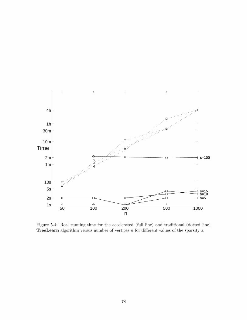
50 100 200 500 1000 1s

2s

5s

10s

1m

2m

10m

30m

1h

4h

s=100 s=100

s=5 s=10 s=15

s=5

s=15 s=10

n

Time

Figure 5-4: Real running time for the accelerated (full line) and traditional (dotted line)TreeLearn algorithm versus number of vertices n for different values of the sparsity s.

78

50 100 200 500 100010

2

103

104

105

106

s=100

s=10 s=5

s=15

n

n Kruskal

Figure 5-5: Number of steps of the Kruskal algorithm nK versus domain size n measuredfor the aCL-II algorithm for different values of s

and 100. The small values were chosen to gauge the advantage of the accelerated algorithmunder extremely favorable conditions. The larger value will help us see how the performancedegrades under more realistic circumstances. Each data point (representing a list of variablesbeing on) was generated as follows: the first variable was picked randomly from the range1, . . . n; the subsequent points were sampled from a random walk with a random step sizebetween -4 and 4. For each pair n, s a set of 10,000 points was generated.

Each data set was used by both TreeLearn and aCL-II to fit one tree distributionand the running times were recorded and plotted in figure 5-4. The improvements over thetraditional version for sparse data are spectacular: learning a tree over 1000 variables from10,000 data points takes 4 hours by the traditional algorithm and only 4 seconds by theaccelerated version when the data are sparse (s = 15). For s = 100 the aCL-II algorithmtakes 2 minutes to complete, improving on the traditional algorithm by a factor of “only”123.

What is also noticeable is that the running time of the accelerated algorithm seems to bealmost independent of the dimension of the domain. On the other side, the number of stepsnK (figure 5-5) grows with n. This observation implies that the bulk of the computationlies with the steps preceding the Kruskal algorithm proper. Namely, that it is in computingcooccurrences and organizing the data that most of the time is spent. This observationwould deserve further investigation for large real-world applications.

Figure 5-4 also confirms that the running time of the TreeLearn algorithm growsquadratically with n and is independent of s.

79

5.8 Concluding remarks

This chapter has presented a way of taking advantages of sparsity in the data to acceler-ate the tree learning algorithm. The ideas introduced have been developed into the twoalgorithms presented without exhausting the number of possible variants.

The methods achieve their performance by taking advantage of characteristics of thedata (sparsity) and of the problem (the weights represent mutual informations) that areexternal to the Maximum Weight Spanning Tree algorithm proper. Here the algorithmshave been evaluated considering that the data sparsity s is a constant. If this is not thecase, however, the actual complexity of the algorithms can be computed easily from thebounds provided here, since the dependence on s is made explicit in each of them.

Moreover, it has been shown empirically that a very significant part of the algorithms’running time is spent in computing cooccurrences. This prompts future work on applyingtrees and mixtures of trees to high-dimensional tasks to focus on methods for structuring thedata and for computing or approximating marginal distributions and mutual informationsin specific domains.

The aCL-II algorithm relies heavily on the fact that most cooccurrences between vari-ables are zero. Given this fact, it can smoothly handle real values for the non-zero cooc-currence counts and even some classes of priors. The aCL-I algorithm is more restrictivein the sense that it requires integer counts and from the present perspective, it is at cleardisadvantage w.r.t aCL-II both in simplicity and in versatility.

5.9 Appendix: Bounding the number of lists NL

Let us denote the total number of nonempty lists V ±c (u), c > 0, u ∈ V by NL. It is obviousNL is maximized when all list lengths are 1 for c ≤ C, 0 for c > C+ 1 and 0 or 1 for c = C,where C is a constant to be determined. In this case, the number of lists can be expressedsuccessively as

NL = nC∑

c=1

2c+O(n)(C + 1)

= n(C + C2) +O(n)(C + 1)

Thereforen(C + C2) ≤ NC ≤ s2N/2 (5.40)

Solving for C we obtain

C ≤ −1

2+

√s2N

2n+ 1 (5.41)

which amounts to

NL = nC +O(n)

= Osn

√N

n

√1

2+

n

s2N

(5.42)

Under the assumption that Nn is bounded above and below the equation simplifies to

NL = O(sn) (5.43)

80

Chapter 6

An Approach to Hidden variablediscovery

Atatea claile de fire stangi!Gasi-vor oare gest inchis sa le rezume,Sa nege, dreapta, linia ce frangi–Ochi ın virgin triunghi taiat spre lume?Ion Barbu–GrupSo many heaps of tangled straw!Will they find clean gesture to comprise them,To straighten them into the golden beamShone by the divine triangle eye?

This chapter presents a way of using mixtures of trees and the MixTreeS learning al-gorithm for discovering structure in a particular class of graphical models with hiddenvariables. In the process of structure discovery model selection and model validation areimportant components. With this goal in mind, I introduce and a novel method for validat-ing independencies in graphical models with hidden variables whose scope is much broaderthan the class of models investigated here.

6.1 Structure learning paradigms

Structure discovery has been one of the most challenging and most fascinating problemsin graphical models ever since the beginning of the field. This is to no surprise given thatthe task of identifying dependencies and independencies in observations is at the core ofscientific discovery as an intellectual process. Work in this field can be loosely categorizedinto three areas of research.

The first category of structure learning methods (and the oldest also) is based on condi-tional independence tests. [68] introduce an algorithm that constructs a Bayesian networkthat is consistent with a given list of independence statements. A similar result exists fordecomposable models: [16] described a method to learn decomposable models or decompos-able approximations to Markov network models using an oracle for conditional independencequeries. The algorithm is exponential in the size of the largest separator. The two works areimpressive in their success in inverting the relationship between a graphical model structureand its list of independencies. On the other hand, the strength of the results reflects thestrength of the underlying assumptions. In other words, the methods assume as input aninformation that is at least as hard to obtain as the graph itself. Testing the conditional

81

independence A ⊥ B | C is exponential in |A|.|B|.|C|. The first method assumes that weknow beforehand all independencies in a domain V (and implicitly all the pairs A,B that arenot independent). But who is to give us such a list of independencies? Moreover, assumingthat we were to undertake the intractable task of performing all the required independencetests, we would be faced with uncertain and perhaps contradictory information that noneof the above methods are prepared to handle.

[55] presents an algorithm for finding a polytree structure from mutual informationmeasurements when the underlying distribution is known to be a polytree. The same chapterpresents a method for learning star decomposable graphs1 the case of binary variables andideal correlation measurements. These methods have the same drawback of requiring idealinformation that cannot be obtained from data.

[6] introduces an algorithm for learning a minimal I-map of a distribution from data.The algorithm is based on evaluation of pairwise mutual informations between variables, andindependence tests that require computational effort proportional to the size of the largestseparator, but it is shown to work efficiently on sparse graphs. The implicit assumptionthat complete independence information can be obtained from pairwise independence tests- an assumption that will be examined later in this chapter. It is also assumed that there issufficient data to ensure a correct answer to all the independence tests, an assumption thatbrings this paper in the same group with the ones requiring ideal information.

The second category of methods explicitly takes into account the existence of a finitesample of data points from which the structure has to be learned. The most influential is theBayesian approach pioneered by [9] and developed by Heckerman, Geiger and Chickeringin the now classical paper [33]. They state the problem of Bayesian learning of Bayesianbelief networks from data, make explicit the assumptions underlying their approach andshow how to calculate, for each network structure E the score Pr[D, E]. The score isthen used for model comparison. They also prove that optimizing the Bayesian score overnetworks structures is NP-hard when each node is allowed to have more than 1 parent.Therefore, both [9] and [33] use a local search: The search algorithms typically generateproposed additions or deletions of an edge from the graph, and these proposed moves areevaluated by computing (an approximation to) the marginal likelihood of the updated graph(exact calculations can be performed in some cases for graphs without hidden nodes). Localsearch is the most common approach to structure learning thus far. Methods based on non-Bayesian scores have been proposed by [47]. The cited works assume that data are completeand that there are no hidden variables. [62] develop a method for scoring equivalence classesof DAGs with hidden variables in the special case when the dependence relationships arejointly Gaussian, augmented by a heuristic search algorithm.

The third category of methods includes methods that also consider learning from data,but are explicitly aimed at finding dependencies. Some of the methods do not attempt toconstruct a complete graphical model, but to find as many dependencies or independenciesas possible. [64] and [17] directly find dependencies in discrete databases by countingcoincidences in subsamples. [34] constructs minimal Markov nets in a heuristic way. Thefirst two methods are aiming at discovering structure in high-dimensional domains, whereapplying more sophisticated algorithms is computationally too expensive. This is a littleexplored area of research, but it is the area where the approach presented here most likelybelongs.

1A star decomposable graph is a tree over the visible domain augmented with some hidden variableswhere each hidden variable has a degree at least 3.

82

The method to be developed in the forthcoming is fundamentally a method of learningfrom data. It belongs to the third category of the above taxonomy by the fact that itis mainly concerned with finding (a certain class of) dependency structures rather than afully determined graphical model. But it relates to the second category by the fact that itgenerates multiple models and compares them by a score that will be further defined.

6.2 The problem of variable partitioning

The approach to structure learning presented in this thesis differs from all the methodsmentioned above. Rather than adopting a local search heuristic based on single edge addi-tion or deletion like the methods in the second category, or than looking for dependencieslike the methods in the third category, it attempts to find separators.

A separator2 is a variable or group of variables S that, when observed, separates V \ Sinto two independent subsets A1, A2. If a separator exists and it is found, then learning thestructure of the domain V reduces to learning the structures of A1

⋃S and A2

⋃S. Since the

number of possible structures grows superexponentially with n, by partitioning the domainthe search space is reduced in a superexponential manner. Moreover, if more separatorscan be found in A1, A2, then one can proceed recursively, effectively implementing a divide-and-conquer structure learning algorithm. We call this approach variable partitioning.

If the separator S is included in V it is called a visible separatore. A visible separatorof small size (practically 1 or 2 variables) can be found in a brute-force manner, by tryingall possibilities. The number of such trials is O(n|S| and each trial implies testing theconditional independence of two or more large sets, an exponential task by itself. As it willbe shown later in this chapter (section 6.7.3), under certain assumptions the aforementionedindependence tests can be reduced to tests on pairs of variables. This makes each trialquadratic in n.

This work focuses on a different situation: the case when the separator is a hiddenvariable. For this case the brute force approach is not sufficient and a different methodneeds to be devised. Much of the machinery developed for this case is applicable to visibleseparators; such that, in some sense, a visible separator is a simple case of hidden variableseparator.

The hidden variable separator, or shortly hidden variable h, is assumed to partitionV into several clusters of variables that are mutually independent conditioned on h. Tomaintain computational tractability, we assume a restrictive architecture for each cluster,in particular we assume that each cluster is a tree. We propose an algorithm whose goalit is to find a good set of trees and to find a good choice of tree structure within eachcluster. Later we examine what happens when the true distribution of the data violatesthis restrictive assumption.

Let V denote as usual the set of variables of interest. Remember also that xv is aparticular value of V, xA an assignment to the variables in the subset A of V and x is ashorthand for xV . The variables in V will be referred to as being visible. We introducean additional variable, a hidden (unobservable) variable denoted by h. This variable takesvalues ranging from 1 to m. The joint space V ∪ h is denoted by V h. The followingassumption about the joint distribution P over V h is essential:

Assumption 1. The hidden variable h partitions V into p mutually disjoint subsets

2The term originates in the junction tree literature.

83

Figure 6-1: The H-model (a) and a graphical model of the same distribution marginalizedover h (b).

h

A1

A2

A1

A2

(a) (b)

A1, . . . , Ap,⋃j Aj = V that are conditionally independent given h. We write

Aj ⊥ Aj′ | h j, j′ = 1, . . . m (6.1)

Consider the graphical model G corresponding to P (figure 6-1,a). Assumption 1 impliesthe graph topology G = (V h, E ∪ E′)3. The edge set is the union of E ′, which contains adirected edge from the hidden variable h to each of the visible variables in V , and of E, whichcontains only undirected edges between pairs of visible variables. Moreover, the inducedgraph over V only has p connected components. Thus, in the graphical model language,conditional independence given h translates into h separating the respective variable clustersin G. We can view this model as a mixture of factorial models over the p hyper-variablesA1,...p. Therefore, we call a model that satisfies Assumption 1 a hyper mixture of factorials,or in short an H model. H models are chain graphs.

Note that Aj being mutually independent given h does not imply that Aj are indepen-dent after marginalizing over the values of h. Graphically, if Aj are mutually separated (byh) in G, they are in general not separated in the graph GM = (V,EM ) corresponding tothe marginal distribution of V

Q(x) =m∑

k=1

P (x, h = k) (6.2)

Let us compute the number of parameters of the models represented by P and Q underthe simplifying assumption that |v| = 2 for all v, p = 2 and that P, PAj |h, j = 1, 2 arerepresented by probability tables. We have

#pars(P ) = m(2|A1|+ 2|A2|− 2) 2n− 1 = #pars(Q) for m 2n/(2|A1 |+ 2|A2|) (6.3)

Hence, if the sizes of A1 and A2 are close, introducing a hidden variable can result inexponential savings in terms of the number of parameters.

We formulate the variable partitioning task as follows: given a domain V h = h⋃j Ajsuch that Aj⊥Aj′ |h ∀j, j′ and a set of observations D = x1, . . . , xN from V =

⋃j Aj, find

the sets Aj , the number of values of h, the distribution Ph and the distribution γi = P (h|xi)over the values of the hidden variable for each of the observed instances xi in D.

Of course, the final goal is to construct a model P of the domain; to do this, oncevariable partitioning is completed, one has two choices: either to use the model P that

3More precisely, a graph that is consistent with Assumption 1 is equivalent to a structure of type G

84

our algorithm learns, or to construct by some other method (including a recursive call toour variable partitioning algorithm) a probabilistic model for each of the domains Aj ∪ h.The sizes of the domains being smaller than n, this task should be considerably easier thanconstructing a model over V directly.

However, one should be aware of the important difficulties that this quest has to face.Searching over the space of all possible partitions of V (of size ∼ pn

p! ) is a forbidding task. Ithas been shown that learning the structure of belief networks from data even in the absenceof hidden variables is an intractable problem [33]. Second, the H model is a mixture modeland we also know that learning mixtures in certain instances is NP-hard [4]. The abovereasons show that all one can do is to provide heuristic procedures for coping with thislarge-scale but important search problem.

There are theoretical difficulties as well: as it has been shown, graphical models withhidden variables do not belong to the curved exponential family and thus the BIC/MDLcriterion is not a consistent estimate of the marginal likelihood of the model structure,as it is for exponential family models [29]. Computing the Bayesian posterior marginalprobabilities of the model structure represents an equally intractable computation.

It is also generally known that models with hidden variables are subject to non-identifiabilityproblems. A simple example will illustrate this: Suppose that the observed distributionover the two binary variables a, b is uniform and that we know that this distribution is themarginal of a mixture distribution

Qab =∑

k=1,2

Ph(k)Pab|h=k

The above is an underdetermined system of equations in the unknowns Ph, Pab|h. Two ofthe possible solutions are

P(1)h (k) = 0.5 k = 1, 2; P

(1)ab|0 =

0 a = b0.5 a 6= b

P(1)ab|1 =

0.5 a = b0 a 6= b

and

P(2)h (k) = 0.5 k = 1, 2; P

(2)ab|0 =

0 a = 00.5 a = 1

P(2)ab|1 =

0.5 a = 00 a = 1

Both of the above distributions have a uniform marginal over a, b and so does any convexcombination of P (1), P (2). Hence there is an infinity of mixture models that have the samemarginal over the observed variables.

Non-identifiability can cause severe convergence problems in learning the model. Forour task identifiability is even more important, since in its absence we are likely to findseveral hidden variable solutions (potentially an infinity!) that explain the data equallywell. Identifiability of hidden variable models is an area of current research [29, 59, 63].The existent results are only preliminaries to a general theory. However, in the case ofmodels with binary variables only, [63] gives the following sufficient condition that is highlyrelevant to the present problem.

Theorem [63] An H-model over a domain V h consisting of binary variables only isidentifiable if either (a) or (b) hold:

(a) p ≥ 3

(b) p = 2, V = A1⋃A2 and PA1|h, PA2|h are not fully connected graphical models.

85

6.3 The tree H model

In the following we present an algorithm for variable partitioning derived under additionalassumptions about the model structure. We shall also assume for now that m and p areknown.

We define a tree H model over V h = h⋃(⋃p

j=1Aj)

as an H model for which PAj |h=k ≡T kAj are trees for all j, k. The structure of T kAj is fixed for all k, but its parameters may vary

with k. We denote the structure of each connected component4 j by Ej . Their union is theedge set E =

⋃j Ej . Because there are p distinct connected components we have

|E| = n− p (6.4)

The conditional distribution

PV |h(x|k) ≡ T k(x) =∏

j

T kAj (xAj )

can be viewed either as the product of p independent trees over the Ajs or as one tree T k

over V having p connected components. This remark enables us: (1) to avoid explicitlyspecifying p from now on by using the notation T k and (2) to view the H as a special caseof mixture of trees with shared structure. This allows us to use the efficient algorithmsdevised for mixtures of trees for fitting tree H models.

A tree H model is obviously a mixture of trees with shared structure; therefore, learningit can be done by a variant of the MixTreeS learning algorithm. The derivation of thealgorithm closely parallels the one given in section 3.3.3, so only the final description thereofis be included here.

Algorithm HMixTreeS

Input: Dataset D = x1, . . . xNProcedure Kruskal( p, weights ) that fits a maximum weight tree with n− p edges over Vp a minimum number of connected componentsInitial model M0

Initialize EM with M = E, λk, T k, k = 1, . . . mIterate until convergence

E step: compute γik, Pk(xi) for k = 1, . . . m, i = 1, . . . N

M step:M1. λk ← Γk/N, k = 1, . . . mM2. compute marginals P kv , P

kuv, u, v ∈ V, k = 1, . . . m

M3. compute mutual information Ikuvu, v ∈ V, k = 1, . . . mM4. call Kruskal(p, Iuv|h) to generate E

M5. T kuv ← P kuv, ;T kv ← P kv for (u, v) ∈ EOutputM

As one can see, the only change w.r.t the standard MixTreeS algorithm is in step M4 wherewe need to construct the maximum weight tree with the prescribed maximum number ofedges. Kruskal’s algorithm fits this purpose easily, since it adds the edges in the order of

4The reader should be aware of the distinction between mixture components indexed by the values of hand connected components which are subtrees of each tree mixture component and are indexed by j = 1, . . . p.

86

their decreasing weight. It can be proved5 that stopping Kruskal’s algorithm after it addsn − p edges results in the maximum weight spanning tree with (at most) that number ofedges.

6.4 Variable partitioning in the general case

6.4.1 Outline of the procedure

We have presented a tractable algorithm for learning a special case of H models, the treeH models. Our next step is to apply the same algorithm to data that are not known to begenerated by a tree H model. Hence, we need to proceed with caution and to use modelselection and validation criteria to evaluate the output of the algorithm.

The procedure I used can be outlined as a two stage process: The first stage generatesmodels with different values for m and p and different structures and parameters by repeat-edly calling the HMixTreeS algorithm. The second stage validates the models producedin the first stage by testing that the independencies they imply are not contradicted bythe data and computes a score for each (valid) model. The different models can be thencompared based on this score. The method is summarized as follows:

Algorithm H-learn – outline

Input: Dataset D = x1, . . . xNConfidence level δParameters mMAX , pMAX , N

trials

Procedure HMixTreeSfor m = 2, 3, . . . ,mMAX

for p = 2, 3, . . . pMAX

for t = 1, . . . , N trials

Initialize randomly M0

Mm,p,t=HMixTreeS(D,M0, p)Validate Mm,p,t with confidence δif Mm,p,t valid

Compute score(Mm,p,t)OutputM = argmin

Mm,p,tvalidscore(Mm,p,t) or the l models with best score

The rest of the chapter studies and develops this approach. For two of the subtasksinvolved - evaluating the description length of a model and testing independence - detaileddescriptions are given in sections 6.6 and 6.7 respectively.

6.4.2 Defining structure as simple explanation

When we set our goal to be learning about a real domain that has inherently unobservedvariables, having little or no prior knowledge about it, how can we know when we havediscovered the “right” interactions between variables ? We shall define a good structure inthis case as a structure that is both simple and likely in view of the data, simplicity beingmeasured by the description length of the model. The reader may have realized already

5By a proof similar to the proof of Theorem 8.2.18. in [71].

87

that we what we have stated is a version of the well known Minimum Description Length(MDL) principle [57].

M∗ = argminM

[

DL(D,M)︷ ︸︸ ︷DL(M) + DL(D|M)] (6.5)

The last term in (6.5) is − logPr[D|M] the negative base 2 log-likelihood. The firstterm can be decomposed as

DL(M) = bits(m) + bits(structure) +m∑

k=1

bits(parameters | structure) (6.6)

Note that any tree structure requires the same number of bits6, independently of p (1 foreach variable, specifying its parent or φ). The first term is also constant over all models7.Hence, computing the description length amounts to computing the description length ofthe parameters for the distributions T k. However, this is not a straightforward task.

We can approach it in two ways. The first is to use the approximation to the modeldescription length derived by Rissanen [57] and also known as the Bayes Information Crite-rion (BIC). It assumes 1

2npars logN as the description length of the parameters. Accordingto BIC, each edge (uv) ∈ ET contributes

∆BICuv =

m

2(ru − 1)(rv − 1) logN (6.7)

bits in addition to the description of a “tree” with no edges that we take as bottom line.The minimization of the DL over tree structures can be automatically incorporated into theEM algorithm, by assigning the weigths

Wuv = NIuv|h −∆BICuv . (6.8)

The method has the advantage of indirectly controling the number of connected componentsp. A drawback of equation (6.8) is that it penalizes parameters in each component equally.To see why this is a problem, imagine that there is one component that is responsible for nodata at all; the parameters of this component will have no influence on the data likelihoodbut the model will still be penalized for them. So, it would be sensible to replace m in theabove formula with something representing an “effective number of parameters”.

A heuristic remedy that I tried for this problem is to take into account the fact thatparameters are estimated from different amounts of data for each k. Hence, I consideredthat each edge (uv) ∈ ET contributes to the total penalty by

∆BIChuv =1

2(ru − 1)(rv − 1)

m∑

k=1

max(log Γk, 0) (6.9)

which gives the BICh criterion.A second approach is to directly approximate the DL of a model. To achieve this, we

represent the probability values on a number of bits b (smaller than the machine precision)obtaining an approximate model Mb. For each b in a chosen range, DL(Mb) is easily

6Unless we have a nonuniform prior over tree structures.7If m is small,as it is implicitly assumed throughout the paper and if there is no prior on m. Otherwise,

the first term will vary with m.

88

computed and so is Pr[D|M]. Then we approximate the true DL by argminb

DL(D,Mb).

A full description of this procedure will be included in section 6.6. This method being apurely evaluatory method, it can be used even for models learned using the penalty fromequations (6.8) or (6.9) above.

Number of connected components p As a consequence of the weight modification(6.8), the weights can now be negative. Kruskal’s algorithm will stop adding edges whenit first encounters a weight ≤ 0, so this implicitly controls p. Moreover, the penalty willbe likely to increase with m thus favoring sparser structures. Alternatively, one can makep vary over a previously fixed range (e.g. between 2 and n) and compare all the resultingmodels by their description lengths.

Selecting m. The description length DL provides us with a consistent criterion forcomparing between model structures with different numbers of trees, thus enabling us toselect m.

Local optima We deal with this problem in the usual way: by restarting the EMalgorithm several times, each time from different random points in the model space. Con-sequently, for each new run of the EM algorithm we may end up with a different modelstructure (and parameters) but this is a help inasmuch as it is a problem, since the role ofthe EM algorithm is to present us with good, but also diverse candidate structures.

6.5 Experiments

6.5.1 Experimental procedure

The experiments described in the following aim to assess the ability of the HMixTreeSalgorithm to discover the correct structure and the hidden variable in two cases: when thedata are generated by a mixture of trees and when they are not. In both cases, we willalso evaluate the description length and the alternative scores discussed above as modelselection criteria for this task.

The experiments therefore were run on artificial data generated in two steps. First,an H-model structure is created (figures 6-2 and 6-3 show the structures used here). Thedomain has 12 visible variables and one hidden variable, all taking 3 values. Second, foreach structure, 10 sets of random parameters were sampled; each resulting model was usedto generate a data set of 3,000 examples, of which 2,000 were used for training and 1,000were used for testing. The values of the hidden variable were recorded but served only fortesting purposes. The first structure (figure 6-2) is a tree H model, the other two (figure6-3) are general H models. In the latter case, because pilot experiments have shown thatdiscovering the variable partitioning is relatively easy when the true partitioning is visiblein the marginal distribution of the data, all the data sets were checked for this propertyand accepted only if the true structure could not be recovered by fitting a single tree.

6.5.2 Experiments with tree H models

This group of experiments demonstrates that the HMixTreeS algorithm is capable ofrecovering structure when the generative model is a tree H model. The model structure isshown in figure 6-2. Two random parametrizations for this structure were generated andfrom each them a training set (N = 3, 000) and a test set (Ntest = 1000).

For each training set, models with m = 2, 3, 4 were learned using the MDL edge penaltyto choose the number of connected components p. For comparison the case m = 3, p =

89

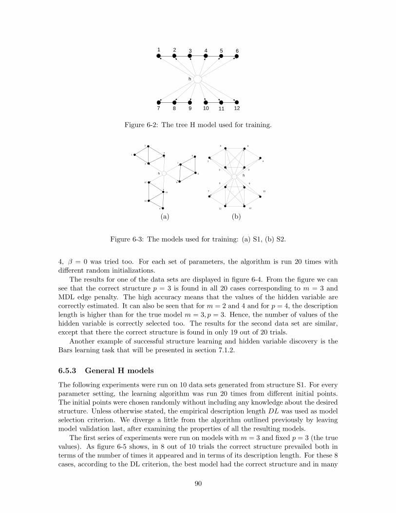
h

1 2 3 4 5 6

7 8 9 10 11 12

Figure 6-2: The tree H model used for training.

h

7

8

9

10

11

12

2

1 5

3

4

6 h

1

2 3

4

7

8 9

10

11 12

5 6

(a) (b)

Figure 6-3: The models used for training: (a) S1, (b) S2.

4, β = 0 was tried too. For each set of parameters, the algorithm is run 20 times withdifferent random initializations.

The results for one of the data sets are displayed in figure 6-4. From the figure we cansee that the correct structure p = 3 is found in all 20 cases corresponding to m = 3 andMDL edge penalty. The high accuracy means that the values of the hidden variable arecorrectly estimated. It can also be seen that for m = 2 and 4 and for p = 4, the descriptionlength is higher than for the true model m = 3, p = 3. Hence, the number of values of thehidden variable is correctly selected too. The results for the second data set are similar,except that there the correct structure is found in only 19 out of 20 trials.

Another example of successful structure learning and hidden variable discovery is theBars learning task that will be presented in section 7.1.2.

6.5.3 General H models

The following experiments were run on 10 data sets generated from structure S1. For everyparameter setting, the learning algorithm was run 20 times from different initial points.The initial points were chosen randomly without including any knowledge about the desiredstructure. Unless otherwise stated, the empirical description length DL was used as modelselection criterion. We diverge a little from the algorithm outlined previously by leavingmodel validation last, after examining the properties of all the resulting models.

The first series of experiments were run on models with m = 3 and fixed p = 3 (the truevalues). As figure 6-5 shows, in 8 out of 10 trials the correct structure prevailed both interms of the number of times it appeared and in terms of its description length. For these 8cases, according to the DL criterion, the best model had the correct structure and in many

90

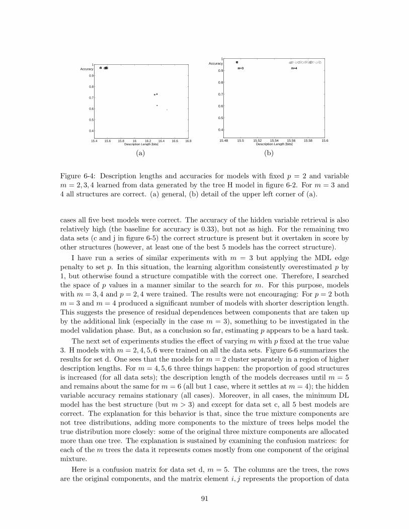
15.4 15.6 15.8 16 16.2 16.4 16.6 16.8

0.4

0.5

0.6

0.7

0.8

0.9

1

Description Length [bits]

Accuracy

15.48 15.5 15.52 15.54 15.56 15.58 15.6

0.4

0.5

0.6

0.7

0.8

0.9

1

m=4m=4m=3m=3

Accuracy

Description Length [bits]

(a) (b)

Figure 6-4: Description lengths and accuracies for models with fixed p = 2 and variablem = 2, 3, 4 learned from data generated by the tree H model in figure 6-2. For m = 3 and4 all structures are correct. (a) general, (b) detail of the upper left corner of (a).

cases all five best models were correct. The accuracy of the hidden variable retrieval is alsorelatively high (the baseline for accuracy is 0.33), but not as high. For the remaining twodata sets (c and j in figure 6-5) the correct structure is present but it overtaken in score byother structures (however, at least one of the best 5 models has the correct structure).

I have run a series of similar experiments with m = 3 but applying the MDL edgepenalty to set p. In this situation, the learning algorithm consistently overestimated p by1, but otherwise found a structure compatible with the correct one. Therefore, I searchedthe space of p values in a manner similar to the search for m. For this purpose, modelswith m = 3, 4 and p = 2, 4 were trained. The results were not encouraging: For p = 2 bothm = 3 and m = 4 produced a significant number of models with shorter description length.This suggests the presence of residual dependences between components that are taken upby the additional link (especially in the case m = 3), something to be investigated in themodel validation phase. But, as a conclusion so far, estimating p appears to be a hard task.

The next set of experiments studies the effect of varying m with p fixed at the true value3. H models with m = 2, 4, 5, 6 were trained on all the data sets. Figure 6-6 summarizes theresults for set d. One sees that the models for m = 2 cluster separately in a region of higherdescription lengths. For m = 4, 5, 6 three things happen: the proportion of good structuresis increased (for all data sets); the description length of the models decreases until m = 5and remains about the same for m = 6 (all but 1 case, where it settles at m = 4); the hiddenvariable accuracy remains stationary (all cases). Moreover, in all cases, the minimum DLmodel has the best structure (but m > 3) and except for data set c, all 5 best models arecorrect. The explanation for this behavior is that, since the true mixture components arenot tree distributions, adding more components to the mixture of trees helps model thetrue distribution more closely: some of the original three mixture components are allocatedmore than one tree. The explanation is sustained by examining the confusion matrices: foreach of the m trees the data it represents comes mostly from one component of the originalmixture.

Here is a confusion matrix for data set d, m = 5. The columns are the trees, the rowsare the original components, and the matrix element i, j represents the proportion of data

91

4.54 4.56 4.58 4.6 4.62 4.64

x 104

0.4

0.5

0.6

0.7

0.8

0.9

1

Description Length [bits]

Accuracy

4.52 4.54 4.56 4.58 4.6 4.62 4.64

x 104

0.4

0.5

0.6

0.7

0.8

0.9

1

Description Length [bits]

Accuracy

4.94 4.95 4.96 4.97 4.98 4.99 5 5.01 5.02

x 104

0.4

0.5

0.6

0.7

0.8

0.9

1

Description Length [bits]

Accuracy

a b c

4.8 4.81 4.82 4.83 4.84 4.85 4.86 4.87 4.88

x 104

0.4

0.5

0.6

0.7

0.8

0.9

1

Description Length [bits]

Accuracy

4.62 4.64 4.66 4.68 4.7 4.72 4.74

x 104

0.4

0.5

0.6

0.7

0.8

0.9

1

Description Length [bits]

Accuracy

4.76 4.78 4.8 4.82 4.84 4.86 4.88

x 104

0.4

0.5

0.6

0.7

0.8

0.9

1

Description Length [bits]

Accuracy

d e f

4.74 4.75 4.76 4.77 4.78 4.79 4.8 4.81

x 104

0.4

0.5

0.6

0.7

0.8

0.9

1

Description Length [bits]

Accuracy

4.68 4.7 4.72 4.74 4.76 4.78

x 104

0.4

0.5

0.6

0.7

0.8

0.9

1

Description Length [bits]

Accuracy

4.78 4.8 4.82 4.84 4.86 4.88

x 104

0.4

0.5

0.6

0.7

0.8

0.9

1

Description Length [bits]

Accuracy

g h i

4.71 4.72 4.73 4.74 4.75 4.76

x 104

0.4

0.5

0.6

0.7

0.8

0.9

1

Description Length [bits]

Accuracy

j

Figure 6-5: Model structures and their scores and accuracies, as obtained by learning treeH models with m = 3 and p = 3 on 10 data sets generated from structure S1. Circlesrepresent good structures and x’s are the bad structures. A + marks each of the 5 lowestDL models. The x-axes measure the empirical description length in bits/example, thevertical axes measure the accuracy of the hidden variable retrieval, whose bottom line is at0.33

92

4.7 4.75 4.8 4.85 4.9 4.95 5 5.05

x 104

0.4

0.5

0.6

0.7

0.8

0.9

1

Description Length [bits]

Accuracy

Figure 6-6: Model structures and their scores and accuracies, as obtained by learning treeH models with p = 3 and variable m = 2, 3, 4, 5 on a data set generated from structure S1.Circles represent good structures and x’s are the bad structures. The sizes of the symbols areproportional to m. The x-axis measures the empirical description length in bits/example,the vertical axis measures the accuracy of the hidden variable retrieval, whose bottom lineis at 0.33. Notice the decrease in DL with increasing m.

from component i modeled by tree j.

0 1 2 3 4

0: 0.504 0.391 0.063 0.018 0.025

1: 0.010 0.018 0.659 0.012 0.301

2: 0.050 0.023 0.045 0.837 0.045

Cluster Accuracy = 0.914

The experiments show that choosing m solely by minimizing the description length canlead to an overestimation of the number of components. Based on the gap in the DLdimension between the models with m = 2 and the rest of the models (all data sets exceptc) one could study the possibility of using it as a criterion for selecting m.

Comparison between the different model section criteria The above results wereplotted again (not shown), replacing in turn the BIC, the modified BIC and the test setlog-likelihood as the horizontal axis, in order to see if there are differences in selecting thecorrect structure. We found that the test log-likelihood fails to select the best model in3 cases when DL does, however we think that this is not sufficient evidence that the log-likelihood is less good than the description length. The other differences seemed also tofavor the empirical description length, but in an even less significant way.

The results obtained for the second structure are qualitatively similar.

93

6.6 Approximating the description length of a model

Here is described the method used to approximate the DL of a mixture of trees model. Itis a general enough method to be used with any probability model, graphical or not. Theidea is to encode the model M as best we can on a fixed number of bits B and then tocompute the description length of the data under this approximated model calledMB. If Bis smaller than the length of the original representation ofM and ifM is a local maximumof the likelihood, then the term DL(D |MB) will be larger then the original DL(D |M);however, the model DL will be equal to B and thus smaller than the original DL(M). Byvarying B over a reasonable range and minimizing the total description length we obtain

DLemp = argminB

DL(D,MB), (6.10)

an upper bound to the local minimum of the desired description length.The better the encoding for each B (in the sense of preserving the likelihood of each

observed data point), the closer is the above minimization to the true DL(D,M). Inpractice, we realize a tradeoff between encoding quality and computational cost. We wantcheap encoding schemes that preserve the represented distribution reasonably well.

To evaluate the DL of a mixture of trees, we use the above idea only to approximatethe DL of the tree parameters within the mixture’s DL. We assume that the structuredescription takes the same number of bits for any tree (n pointers, one – possibly null – forthe parent of each node) and thus can be ignored from the DL. The DL of the λ parametersis approximated by

bλ =m− 1

2logN.

The parameters of the tree distributions are encoded with the same number of bits b. Thisnumber is a sum of two precisions, bm and bM , that will be defined below. The numberof parameters is given by equation (2.7). Thus, the total number of bits (excluding theconstant for structure) is

DL(Q) = bλ +m(bm + bM )[∑

(u,v)∈E(ru − 1)(rv − 1) +

∑

v∈Vrv − n] +

∑

(u,v)∈Eru log rv (6.11)

Now we show how to encode the parameters of the trees. In our directed tree based im-plementation, the parameters represent the values of the conditional probabilities Tv|pa(v)(xv|xpa(v))(where, of course, sometimes pa(v) is the empty set). For each fixed value of pa(v), thisdistribution is a multinomial. Therefore, in the following we describe a way of encodingmultinomial distribution.

6.6.1 Encoding a multinomial distribution

Encoding a set of real numbers on a finite number of bits always involves some sort ofquantization. So, to encode the parameters of a distribution one needs to first quantizethem. The quantization of the multinomial distribution parameters is done in the naturalparametrization introduced in section 4.2.2.

Let the distribution values be θj, j = 1 . . . r and let jMAX be the index of the largest θ.The natural parameters are given by (4.27), reproduced here in slightly modified form

φi = − log θilog θr

i = 1, . . . r, i 6= jMAX . (6.12)

94

Adding a minus sign in front of the logarithm function ensures that all the φ parametersare positive. Since the θ parameters are allowed to be 0, their range is in [0,∞].

We are going to represent the φ values on a finite number of bits. This is done in twostages: First, the large φ values are “truncated” to the constant 2bM if they exceed it. Thiscorresponds to bounding the smallest θ values away from 0. Then, the resulting values arerepresented as bm bit precision binary numbers, or equivalently, they are multiplied by 2bm

and stored as integers. Note that while bM controls the representation precision for smallprobabilities, bm control the precision of large probabilities. Both precisions are relative tothe largest value of θ. The full encoding of θ1...r is represented by r, the encoding precisionbm, the position of the maximum jMAX and the values

φenci = 2bm min(φi, 2bM ), i = 1, . . . r, i 6= jMAX (6.13)

To decode the values of θ from the above representation one has to apply formula (4.28)to φenci 2bm and replace the maximum θ in position jMAX . Note that the value bM is notnecessary for decoding.

If the value of r is given by a separate table (remember that we are encoding severaldistributions over the same domain) and that bm is also encoded separately, the total numberof bits to encode θ1,...r is

logdre+ (bm + bM )(r − 1) ≈ log r + (bm + bM )(r − 1) (6.14)

By adding up the right-hand sides of (6.14) values for all Tv|pa(v) one obtains the last twoterms of (6.11). To see this remark that: (1) each free parameter is encoded on bM +bm bitsand (2) ru log rv = rv log ru for all positive numbers ru, rv. To make the search tractable,the values of bm and bM are common to all distributions in Q and thus bm is recorded onlyonce.

6.7 Model validation by independence testing

6.7.1 An alternate independence test

Assume that we have two independent discrete variables u and v taking ru, rv values re-spectively, and an i.i.d. sample of size N drawn from their joint distribution. Since thevariables are independent, their mutual information is obviously zero, but its estimate fromthe sample Iuv does not generally exactly equal zero. In this section we want to bound theprobability that the sample mutual information Iuv is larger than a threshold M > 0.

Of course, Iuv will never exceed max(log ru, log rv) so it will be assumed that M is belowthis value. We shall use large deviation theory, and in particular Sanov’s theorem [11] toobtain this bound.

Let us denote by Puv, Pu, Pv respectively the sample joint distribution of u, v and itsmarginals. We shall consider the following two sets of probability distributions over thedomain Ω(uv)

E = P | IPuv ≥M (6.15)

F = Q | IQuv = 0 (6.16)

The set F represents all the factorized distributions over Ω(uv). With this notation ourproblem can be formulated as: what is the probability of the sample distribution P tobelong to E given that the true distribution is in F ?

95

Sanov’s theorem gives us the following result: For any distribution Q and any closedset of probability distributions E, the probability that the sample distribution P of an i.i.d.sample of size N drawn from Q is in E is denoted by QN (E) and satisfies

QN (E) ≤ (N + 1)r2−N.KL(P ∗Q ||Q) (6.17)

where r is the size of Q’s domain and

P ∗Q = argminP∈E

KL(P ||Q) (6.18)

is the distribution in E that is closest to Q in KL-divergence8. We also know [72] that forany distribution P over Ω(uv)

minQ∈F

KL(P ||Q) = KL(P ||PuPv) = IPuv. (6.19)

Hence

minP∈E,Q∈F

KL(P ||Q) = minP∈E

IPuv = M (6.20)

Using this result in Sanov’s theorem above we conclude that for any Q ∈ F

QN (E) ≤ (N + 1)rurv2−NM (6.21)

In other words, for any two independent variables u, v, the probability that their samplemutual information Iuv exceeds a threshold M > 0 is bounded by

(N + 1)rurv2−NM = δ.

Conversely, given a probability δ we can derive the corresponding M :

M =1

N[log

1

δ+ rurv log(N + 1)] (6.22)

This bound is distribution free: it requires no assumption about the distributions of u andv. As expected, the value of M for fixed δ decreases with the sample size N . Contrast thiswith the χ2 test, that does make assumptions about the underlying distribution but whosep-values (the analogues of M) are independent of the sample size.

Because E is the closure of its interior, Sanov’s theorem and a reasoning similar to theabove one enables us to establish a lower bound for QN (E)

QN (E) ≥ 1

(N + 1)rurv2−NM (6.23)

It is interesting to compare the test devised here, call it Sanov test with the well-knownχ2 test for independence. It is easy to show that the χ2 statistic is approximating a KLdivergence. For this, let us compute the quantity KL(PuPv || Puv) as a function of thecounts Nij =#times u = i, v = j, Ni =#times u = i, Nj =#times v = j and

nij =NiNj

N, i = 1, . . . ru, j = 1, . . . rv.

8A somewhat tighter bound for the r.h.s of equation (6.17) is [r +N r−1]2−N.KL(P∗Q||Q).

96

KL(PuPv || Puv) =∑

ij

nijN

lognijNij

(6.24)

= − 1

N ln 2

∑

ij

nij lnNij

nij(6.25)

= − 1

N ln 2

∑

ij

Nij ln(1 +Nij − nij

nij) (6.26)

≈ − 1

N ln 2

∑

ij

[nijNij − nij

nij− 1

2nij

(Nij − nij)2

n2ij

+ . . .] (6.27)

=1

N ln 2

1

2

∑

ij

(Nij − nij)2

nij(6.28)

=1

2 ln 2χ2 (6.29)

Hence, whereas the Sanov test is based on KL(Puv || PuPv), the χ2 independence test isan approximation of the reverse divergence KL(PuPv || Puv). Of course, the motivation forthe χ2 test is not in this divergence but in Central Limit Theorem arguments.

6.7.2 A threshold for mixtures

Now we undertake to estimate an approximate confidence interval for the sample mutualinformation when the variables u and v are independent given a third variable z. In thiscase the true joint distribution of u, v is

Q =m∑

k=1

λkQkuQ

kv (6.30)

where, as usual, the values λk represent the probabilities of variable z being in state k ∈1, . . . m. Again, we assume an i.i.d. sample of size N ; given this sample, we group thedata points by the values of z in m groups of size Nk respectively. Therefore, we have

m∑

k=1

Nk = N.

We denote by Ikuv the sample mutual information between u and v in group k. Let usfurther denote by ρ(N,M) the probability that the sample mutual information from a sizeN sample does not exceed M > 0.

ρ(N,M) = 1−QN (E) (6.31)

Of course, ρ is also a function of ru, rv and the true distribution Q. To simplify the notationwe drop these variables. This is acceptable because ru and rv are fixed and because thedependence on Q will be masked by the use of bounds that hold for any Q.

Our goal is now to fix a confidence level δ and to find the thresholds Mk, k = 1, . . . mdepending on δ such that Ikuv < Mk for all k with probability δ. We start by expressing theprobability of the event E=“Ikuv < Mk for all k” as a function of the values Mk and afterwe arrive at a convenient expression we will equate that with δ.

97

Let us first introduce some notation: let Z be the i.i.d. sample of size N representingthe values of z, and N = (N1, . . . Nm) an m-tuple of Nk values as defined above. By

(NN

)=

N !

N1!N2! . . . Nm!(6.32)

we denote “N choose N1, . . . Nm”, the multinomial coefficient indexed by N = (N1, . . . Nm).Then,

Pr[E ] =∑

Z

Pr[Z]∏

k

Pr[Ikuv < Mk | Z]

=∑

Z

∏

k

λNk(Z)k ρ(Nk(Z),Mk)

=∑

N

(NN

)∏

k

λNkk∏

k

ρ(Nk,Mk)

If the factors ρ(N,M) vary slowly with N (further on we show when this happens), then

the above sum is dominated by the term corresponding to the largest

(NN

)∏k λ

Nkk , a value

attained forN∗k ≈ λkN, k = 1, . . . m. (6.33)

Moreover, using Stirling’s approximation N ! ≈(Ne

)Nwe have

(NN∗

)∏

k

λN∗kk =

N !∏k(λkN)!

∏

k

λλkNk

=N !

NN

∏

k

(λkN)λkN

(λkN)!

≈ e−N+∑

kNλk

= 1

This allows us to write

Pr[E ] ≈m∏

k=1

ρ(Nλk,Mk) (6.34)

If we now choose Mk according to (6.22) i.e.

Mk =1

λkN[log

1

δ+ rurv log(λkN + 1)] (6.35)

we have

1− δ ≤ ρ(λkN,Mk) ≤ 1− δ

(λkN + 1)rurv(6.36)

andPr[E ] ≈ (1− δ)m = 1− δ (6.37)

For a given δ the corresponding δ is

δ = 1− (1 − δ) 1m ≈ δ

m(6.38)

98

To conclude, we have to prove our assumption that the functions ρ(Nk,Mk) vary slowlywith the first argument. More precisely, we are interested in upper bounding them. But

ρ(Nk,Mk)

ρ(N∗k ,Mk)≤ 1

ρ(N∗k ,Mk)≤ 1

1− δ(6.39)

For small values of δ the above quantity is close to unity validating our previous derivation.

6.7.3 Validating graphical models with hidden variables

In this section we will apply the previous test to the models of interest to us: graphicalmodels with a hidden variable that separates the observed ones into two conditionallyindependent subsets. Thus, we will assume that we have a set of variables V , a datasetD = x1, . . . xN of observations from V and the model

Q(x) =m∑

k=1

λkTkA(xA)T kB(xB) (6.40)

where A,B is a partition of V . Thus Q assumes that there is a hidden variable z takingvalues k = 1, . . . m with probabilities λk and that A ⊥ B | z. We want to test whetherthe data D supports the independence implied by Q. In the following we will be referringto the Sanov test developed in section 6.7.1, but arguments similar to those presented herehold for the χ2 independence test.

There are two issues that need to be addressed: First, in this case the variable z isnot observed. Therefore, we use Monte Carlo sampling from the posterior γk(i) to obtainsequences Z = (z1, . . . zN ). For each of them we compute Ikuv, k = 1, . . . m and comparethem to the respective thresholds.

Second, establishing independence between two sets of variables implies a summationover Ω(A) × Ω(B) = Ω(V ). This configuration space is usually much larger than the sizeN of the available sample. With rurv = |Ω(V )| the threshold M becomes giant (6.22) andthe comparison meaningless. And, if N becomes comparable to Ω(V ) then the calculationsbecome intractable. Therefore, we will test the independence of A and B by performingindependence tests on pairs of variables u ∈ A, v ∈ B. In general it is not true that

u ⊥ v | z ∀u ∈ A, v ∈ B =⇒ A ⊥ B | z. (6.41)

But (6.41) is true for a broad class of distributions. In particular, if the true distributionof the data is a chain graph (6.41) holds. Now we have to test the independence of |A||B|pairs of variables, something that is computationally intensive, but tractable. However, wewill be performing simultaneous tests and we have to take this into account.

We use therefore a Bonferroni inequality [42] that states that if each hypothesis Huv istrue with confidence 1− εuv, then their conjunction is true with confidence at least

1−∑

uv

εuv.

In the present case, Huv represent the hypotheses “u ⊥ v | z”; by Euv we denote the events“Ikuv(Z,D) < Mk ∀k”. There is no special reason to treat any of them differently; hence

εuv =ε

|A||B| = ε ∀u ∈ A, v ∈ B (6.42)

99

The test procedure can be summarized as follows:

Algorithm TestIndependenceInput model Q, data set D, confidence ε1. ε = ε/(|A||B|)

fix δ, compute δ by (6.38)2. compute γ = (γk(i), k = 1, . . . m, i = 1, . . . N) the posterior

probability that xi was generated by component k of the mixture3. for u ∈ A, v ∈ B

3.1 compute the thresholds Mk by (6.22)3.2 repeat

3.2.1 sample Z from γ

3.2.2. for k = 1, . . . m compute Ikuv and compare to Mk until

Pr[Euv] <> δ with confidence 1− ε; “>” means reject Huv,“<” means accept it

Output accept independence hypothesis if all the tests in step 3. accept it,otherwise reject

The crux of the method is step 3 where we need to estimate the low probabilities Pr[Euv]with very high confidence ε for each pair u, v. We have of course the freedom to choose aδ closer to 0.5 in order to require fewer iterations of 3.1–3.3 to compare Pr[Euv] with δ atthe required confidence level. But a larger δ means a lower threshold Mk and this in turnmeans loosening the approximation in Sanov’s theorem9 and thus increasing the probabilityof type I error (false acceptance).

The choice of ε reflects our tradeoff between type I and type II errors. For a small εthe probability of rejecting a model (i.e. rejecting the independence hypothesis) that iscorrect is low, but we are likely to accept independence when this is not true. This latterprobability is inflated in our case by further dividing ε between the |A||B| tests in (6.42).Therefore it is better to accept a somewhat larger false rejection risk by choosing a largerε lest the test becomes too permissive.

Let us examine if the assumptions our tests are based upon are true in the aboveprocedure. The |A||B| individual independence tests are dependent on each other becausethey share the observed values (x1, . . . xN ), but the Bonferroni inequality accounts for that.The dataset D is not the dataset the model was trained on.

It is in using an independence test based on Pr[Euv] that we depart from the assump-tions. Because the data D are already observed, the quantity that is actually estimated byrepeating 3.2.1 – 3.2.2 is not Pr[Euv] but Pr[Euv|D]. It can be expressed as

Pr[Euv|D] =∑

Z

Pr[Z|D]∏

k

Pr[Ikuv < Mk|Z,D] (6.43)

=∑

Z

∏

i

γzi(i)∏

k

δIkuv(Z,D)<Mk(6.44)

=∑

Z:Ikuv(Z,D)<Mk ∀k

∏

i

γzi(i) (6.45)

Hence, a correct test would predict or bound the above probability. But this involves theintractable summation over Ikuv(Z,D) < Mk ∀k.

Finally, a general fact about independence tests and their utility. The independencetest can only reject independence and provide an estimate of the risk in doing it. It can

9This can be seen by examining the proof of Sanov’s theorem.

100

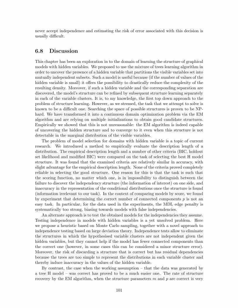
never accept independence and estimating the risk of error associated with this decision isusually difficult.

6.8 Discussion

This chapter has been an exploration in to the domain of learning the structure of graphicalmodels with hidden variables. We proposed to use the mixture of trees learning algorithm inorder to uncover the presence of a hidden variable that partitions the visible variables set intomutually independent subsets. Such a model is useful because (if the number of values of thehidden variable is small) it offers the possibility to drastically reduce the complexity of theresulting density. Moreover, if such a hidden variable and the corresponding separation arediscovered, the model’s structure can be refined by subsequent structure learning separatelyin each of the variable clusters. It is, to my knowledge, the first top down approach to theproblem of structure learning. However, as we stressed, the task that we attempt to solve isknown to be a difficult one. Searching the space of possible structures is proven to be NP-hard. We have transformed it into a continuous domain optimization problem via the EMalgorithm and are relying on multiple initializations to obtain good candidate structures.Empirically we showed that this is not unreasonable: the EM algorithm is indeed capableof uncovering the hidden structure and to converge to it even when this structure is notdetectable in the marginal distribution of the visible variables.

The problem of model selection for domains with hidden variable is a topic of currentresearch. We introduced a method to empirically evaluate the description length of adistribution. The empirical description length and a number of other criteria (BIC, holdoutset likelihood and modified BIC) were compared on the task of selecting the best H modelstructure. It was found that the examined criteria are relatively similar in accuracy, withslight advantage for the empirical description length. None of the criteria proved completelyreliable in selecting the good structure. One reason for this is that the task is such thatthe scoring function, no matter which one, is in impossibility to distinguish between thefailure to discover the independency structure (the information of interest) on one side, andinaccuracy in the representation of the conditional distributions once the structure is found(information irrelevant to our task). In the context of comparing models by score, we foundby experiment that determining the correct number of connected components p is not aneasy task. In particular, for the data used in the experiments, the MDL edge penalty issystematically too strong, biasing towards models with false independencies.

An alternate approach is to test the obtained models for the independencies they assume.Testing independence in models with hidden variables is a yet unsolved problem. Herewe propose a heuristic based on Monte Carlo sampling, together with a novel approach toindependence testing based on large deviation theory. Independence tests allow to eliminatethe structures in which the hypothesised variable clusters are not independent given thehidden variables, but they cannot help if the model has fewer connected components thanthe correct one (however, in some cases this can be considered a minor structure error).Moreover, the risk of discarding a structure that is correct but has residual dependenciesbecause the trees are too simple to represent the distributions in each variable cluster andthereby induce inaccuracy in the values of the hidden variable.

By contrast, the case when the working assumption – that the data was generated bya tree H model – was correct has proved to be a much easier one. The rate of structurerecovery by the EM algorithm, when the structure parameters m and p are correct is very

101

high, often 100%. Likewise, the accuracy of the values of the hidden variable is very good.For model selection with fixed m and p, as well as for search across values of m, p, the modelselection criteria, be they empirical DL or others, are found to be reliable.

102

Chapter 7

Experimental results

This section describes the experiments that were run in order to assess the capabilitiesand usefulness of the mixture of trees model. The first experiments examine the ability ofthe MixTree algorithm to recover the original distribution when the data are generatedby a mixture of trees. For these models, only artificial data are used. The next group ofexperiments studies the performance of the mixture of trees as a density estimator; thedata used in these experiments are not generated by mixtures of trees. Finally, we performclassification experiments. In these experiments, we study both the mixture of trees and aclassifier consisting of a single tree trained as a density estimator. Comparisons are madewith classifiers trained in both supervised and unsupervised mode. The section ends witha discussion of the single tree classifier and its feature selection properties.

In all the experiments below, unless otherwise stated, the training algorithm is initializedat random, independently of the data or of the knowledge about the desired solution. Log-likelihoods are expressed in bits/example1 and therefore are sometimes called compressionrates. The lower the value of the compression rate, the better the fit to the data.

In the experiments that involve small data sets, a smoothing procedure has sometimesbeen used. The technique I applied is called smoothing with the marginal and is describedin [24, 53]. One computes the pairwise marginal distributions for the whole data set P total

uv

and replaces the marginals P kuv by

P kuv = (1− α)P kuv + αP totaluv (7.1)

Intuitively, the effect of this operation is to give a small probability weight to unseen in-stances and to make the m trees more similar to each other, thereby reducing the effectivemodel complexity. For the method to be effective in practice, α is a function of Γk andP kuv. In particular, for the experiments in this thesis, a global smoothing parameter α is ap-portioned between mixture components and, within each mixture component, beween treeedges. Whereas α in the above equation is always between 0 and 1, the global smoothingparameter may be larger than 1. In some cases (e.g. when fitting a single tree), I usedsmoothing with a uniform distribution instead of smoothing with the marginal.

7.1 Recovering the structure

7.1.1 Random trees, large data set

For the first experiment, we generated a mixture of 5 trees over 30 variables with r = 4for all vertices. The distribution of the choice variable λ as well as each tree’s structure

11 bit is the negative base 2 logarithm of a likelihood of 0.5.

103

Figure 7-1: Eight training examples for the bars learning task.

and parameters were sampled at random. The mixture was used to generate 30,000 datapoints that were used as training set for a MixTree algorithm. The initial model hadm = 5 components but otherwise was random. We compared the structure of the learnedmodel with the generative model and computed the likelihoods of both the learned and theoriginal model on a test dataset consisting of 1000 points.

The results on retrieving the original trees were excellent: out of 10 trials, the algorithmfailed to retrieve correctly only 1 tree in 1 trial. This result can be accounted for by sam-pling noise; the tree that wasn’t recovered had a λ of only 0.02. Instead of recovering themissing tree, the algorithm fit two identical trees to the generating tree with the highestλ. The difference between the log likelihood of the samples of the generating model andthe approximating model was 0.41 bits per example. On all the correctly recovered trees,the approximating mixture had a higher log likelihood for the sample set than the gener-ating distribution. This shows that not only the structure but the whole distribution wasrecovered correctly.

7.1.2 Random bars, small data set

The “bars” problem is a benchmark structure learning problem in neural network unsuper-vised learning algorithms. It has many variants, of which I describe the one used in thepresent experiments.

The domain V is the l × l square of binary variables depicted in figure 7-1. The dataare generated the following manner: first, one flips a fair coin to decide whether to generatehorizontal or vertical bars; this represents the hidden variable in our model. Then, eachof the l bars is turned on independently (black in figure 7-1) with probability pb. Finally,noise is added by flipping each bit of the image independently with probability pn.

A learner is shown data generated by this process; the task of the learner is to “discover”the data generating mechanism.

What would it mean to discover the data generating mechanism with a mixture of trees?A mixture of trees model that approximates the true structure (figure 7-2) for low levelsof noise is shown in figure 7-3. Note that any tree over the variables forming a bar is anequally good approximation. Thus, we will consider that structure has been discoveredwhen the model learns a mixture with m = 2, each T k having l connected components, onefor each bar. Additionally, we shall test the “classification accuracy” of the learned model

104

Horiz/Vert

0.5

Pb | 0

(1-Pn) | Pn

(1-Pn) | Pn

0 | Pb

hiddenvariables

visiblevariables

Figure 7-2: The true structure of the probabilistic generative model for the bars data.

hh h=1 =0

Figure 7-3: A mixture of trees approximate generative model for the bars problem. Theinterconnection between the variables in each “bar” are arbitrary.

105

.0001 .01 1 100 100008

10

12

14

16

18

20

Smoothing value

Tes

t lik

elih

ood

[bits

/cas

e]

m=2

m=3

Figure 7-4: Test set log-likelihood on the bars learning task for different values of thesmoothing α and different m. Averages and standard deviations over 20 trials.

by comparing the true value of the hidden variable (i.e. “horizontal” or “vertical”) with thevalue estimated by the model for each data point in a test set.

We do not compare all of our results directly against neural network results, mainlybecause most of the published results are qualitative, focusing on whether the model is ableto learn the structure of the data. We closely replicate the experiment described in [15] in away that makes the present experiment slightly more difficult than theirs. The training setsize is Ntrain = 400 (in [15] it is 500), the data set contains ambiguous examples (exampleswhere no bars are present, which consequently are ambiguous from the point of view ofclassification) and the noise level is small but not zero (it is zero in [15]). Because the otherauthors studying this problem assume incomplete knowledge of structure (in this case, thenumber of hidden units of the neural net), we do something similar: we train models withm = 2, 3, . . . and choose the final model by the likelihood on a holdout set. Typical valuesfor l in the literature are l = 4, 5 (the problem becomes harder with increasing l); we choosel = 5 following [15]. The probabilities pb and pn are 0.2 and 0.02 respectively. The test setsize is Ntest = 200. To obtain trees with several connected components we use a small edgepenalty β = 5. Because the data set is small smoothing with different values for α is used.For each value of m we run the MixTree learning algorithm 20 times on the same trainingset with different random initial points and average the results.

Selection of m The average test set log-likelihoods (in bits) for m = 2, 3 are given infigure 7-4, together with their standard deviations. Clearnly, m = 2 is the best model.

Structure recovery. For m = 2 we examined the resulting structures: in 19 out of 20trials, structure recovery was perfect (in the sense explained above); in the remaining trialthe learned model missed the correct structure altogether, converging to a different localminimum apparently closer to its initial point. For comparison, [15] examined two trainingmethods and the structure was recovered in 27 and respectively 69 cases out of 100. This

106

Table 7.1: Results on the bars learning task.

Test set ambiguous unambiguous

ltest [bits/datapt] 9.82 ± 0.95 13.67 ± 0.60Class accuracy 0.852 ± 0.076 0.951 ± 0.006

Figure 7-5: An example of a digit pair.

result held for the whole range of the smoothing parameter α.Classification. The classification performance is shown in table 7.1. The result re-

ported is obtained for a value of α chosen based on the test set log-likelihood. Note thaton data generated by the previously described mechanism, no model can achieve perfectclassification performance. This is due to the “ambiguous” examples, like the one shown infigure 7-1 (upper row, third from left), where no bars are on (or, less likely, where all barsare on). The probability of an ambiguous example for the current value of pb is

pambig = plb + (1− pb)l = 0.25 (7.2)

Since ambiguous examples appear in either class with equal probability, the error ratecaused by them is 0.5pambig = 0.125. Comparing this theoretical upper bound with thevalue in the corresponding column of table 7.1 shows that the model has indeed a very goodclassification performance, even trained on ambiguous examples.

To further support this conclusion, a second test set of size 200 was generated, thistime including only non-ambiguous examples. The classification performance, shown in thecorresponding section of table 7.1 rose to 0.95. The table also shows the likelihood of the(test) data given the learned model. For the first, “ambiguous” test set, this is 9.82, 1.67bits away from the true model entropy of 8.15 bits/data point. For the “non-ambiguous”test set, the compression rate is significantly worse, no surprise since the distribution of thetest set is now different from the distribution the model was trained on.

7.2 Density estimation experiments

7.2.1 Digits and digit pairs images

We tested the mixture of trees as a density estimator by running it on a subset of binaryvector representations of handwritten digits and measuring the average log-likelihood. Thedatasets consist of normalized and quantized 8x8 binary images of handwritten digits madeavailable by the US Postal Service Office for Advanced Technology. One data set (thatwe call “digits”) contained images of single digits in 64 dimensions, the second (called“pairs” hitherto) contained 128 dimensional vectors representing randomly paired digitimages. Figure 7-5 displays an example of a digit pair. The training, validation and test

107

Table 7.2: Average log-likelihood (bits per digit) for the single digit (Digit) and doubledigit (Pairs) datasets. Boldface marks the best performance on each dataset. Results areaveraged over 3 runs.

m Digits Pairs

16 34.72 79.2532 34.48 78.9964 34.84 79.70

128 34.88 81.26

set contained 6000, 2000, and 5000 exemplars respectively. The data sets, the trainingconditions and the algorithms we compared with are described in [21]. Each model istrained on the same training set until the likelihood of the validation set stops increasing.We tried mixtures of 16, 32, 64 and 128 trees, fitted by the basic algorithm. For each of thedigits and pairs datasets we chose the mixture model with the highest log-likelihood on thevalidation set and using it we calculated the average log-likelihood over the test set (in bitsper example). The averages (over 3 runs) are shown in table 7.2. Notice the small differencein test likelihood between models that is due to early stopping in the training algorithm.

In figure 7-6 we compare our result (for m = 32) with the results published by [21].Theother algorithms plotted in the figure are the mixture of factorial distributions (MF), thecompletely factored model (which assumes that every variable is independent of all theothers) called “Base rate” (BR), the Helmholtz Machine trained by the wake-sleep algorithm[21] (HWS), the same Helmholtz Machine where a mean field approximation was used fortraining (HMF) and a fully visible and fully connected sigmoid belief network (FV). Table7.2 displays the performances of all the mixture of trees models that we tested.

The results are very good: the mixture of trees is the absolute winner for compressing thesimple digits and comes in second as a model for pairs of digits. A comparison of particularinterest is the comparison in performance between the mixture of trees and the mixture offactored distribution. In spite of the structural similarities, the mixture of trees performssignificantly better than the mixture of factorial distribution indicating that there existssome structure that is exploited by the mixture of spanning trees but can’t be captured bya mixture of independent variable models. Comparing the values of the average likelihood inthe mixture of trees model for digits and pairs we see that the second is more than twice thefirst. This suggests that our model (just like the mixture of factored distributions) is ableto perform good compression of the digit data but is unable to discover the independencein the double digit set.

7.2.2 The ALARM network and data set

The second set of density estimation experiments features the ALARM network [33, 6].This Bayes net model is a benchmark model for structure learning experiments. It is amedical diagnostic alarm message system for patient monitoring and it was constructedfrom expert knowledge. The domain has n = 37 discrete variables taking between 2 and 4values, connected by 46 directed arcs. Since the ALARM net was not constructed from acomplete data set I use in the experiments data generated from the model itself. This isartificial data, but it is an interesting experiment for two reasons: (1) the data generating

108

BR MF gzip HWS HMF FV MT 0

10

20

30

40

50

60

Like

lihoo

d [b

its/d

igit]

BR MF gzip HWS HMF FV MT 0

20

40

60

80

100

120

Like

lihoo

d [b

its/d

igit]

(a) (b)

Figure 7-6: Average log-likelihoods (bits per digit) for the single digit (a) and double digit(b) datasets. MT is a mixture of spanning trees, MF is a mixture of factorial distributions,BR is the base rate model, HWS is a Helmholtz machine trained by the Wake-Sleep algo-rithm, HMF is a Helmholtz machine trained using the Mean Field approximation, FV isfully visible fully connected sigmoidal Bayes net. Notice the difference in scale between thetwo figures.

distribution is not a tree or a mixture of trees (17 nodes have more than one parent) butthe topology of the DAG is sparse suggesting that the dependence can be approximated bya mixture of trees with a small number of components m; (2) the generative model capturesthe features of a real domain of practical importance.

We generated a training set having Ntrain = 10, 000 data points and a separate test setof Ntest = 2, 000 data points. On these sets we train and compare the following models:mixtures of trees, mixtures of factorial distributions, the true model (without training),gzip (without training). For mixtures of trees and factorial distributions, the comparison ismade in the following way: we separate a validation set of Nvalid = 1, 000 data points fromthe training set; then, models with different values of m are trained on the remaining dataand evaluated (after the training process converges) on the validation set. For each valueof m we run 20 trials. The averaged value of the log-likelihood on the validation set is usedto choose the optimal m. Then, the models with that m are evaluated on the test set andthe likelihood achieved on it is compared against other classes of models.

The results are presented in table 7.3. The result reported for gzip was obtained bywriting the data in a file in binary format, with all additional information removed andpresenting it to the gzip program.

One can see that, even with a 9,000 data set, the mixture of trees does not approximatethe true distribution perfectly. However, note the difference in likelihood values for the truemodel between the training and the test set, suggesting that a data set in the thousandsis still not a large data set for this domain. Among the other models used to approximatethe true distribution, the mixture of trees is a clear winner. If being ahead of gzip and thebase rate model was expected, it was not so with the mixture of factorials. However, thesuperiority of the mixture of trees w.r.t this model is also clear.

To examine the sensitivity of the algorithms to the size of the data set also ran theexperiment with a training set of size 1,000. The results are presented in table 7.4.

Again, the mixture of trees is the closest to the true model, beatingthe mixture of

109

Table 7.3: Density estimation results for the mixtures of trees and other models on theALARM data set. Training set size Ntrain = 10, 000. Average and standard deviation over20 trials.

Model Train likelihood Test likelihood[bits/data point] [bits/data point]

ALARM net 13.148 13.264Mixture of trees m = 18 13.51 ±0.04 14.55 ± 0.06Mixture of factorials m = 28 17.11 ± 0.12 17.64 ± 0.09Base rate 30.99 31.17gzip 40.345 41.260

Table 7.4: Density estimation results for the mixtures of trees and other models on a dataset of size 1000 generated from the ALARM network. Average and standard deviation over20 trials.

Model Train likelihood Test likelihood[bits/data point] [bits/data point]

ALARM net 13.167 13.264Mixture of trees m = 2, α = 50 14.56 ±0.16 15.51 ± 0.11Mixture of factorials m = 12, α = 100 18.20 ± 0.37 19.99 ± 0.49Base rate 31.23 ± 0.21 31.18 ± 0.01gzip 45.960 46.072

110

factorials by an even larger margin than for the large data set. Notice that the degradationin performance for the mixture of trees is relatively mild (about 1 bit), whereas the modelcomplexity is reduced drastically (from 18 to only 2 mixture components, and this in thecontext of additional parameter smoothing!). This indicates the important role played bythe tree structures in fitting the data and motivates the advantage of the mixture of treesover the mixture of factorials for this data set.

7.3 Classification with mixtures of trees

7.3.1 Using a mixture of trees as a classifier

Classification is a common and important task for which probabilistic models are often used.Very often density models are trained on data with the sole purpose of classification. Thisprocedure is not asymptotically optimal, but there is empirical evidence that it can offergood performance in practice. Therefore, this section will be devoted to experimentallyassessing the performance of the mixture of trees model in classification tasks.

A density estimator can be turned into a classifier in two ways, both of them beingessentially likelihood ratio methods. Denote the class variable by c and the set of inputvariables by V . In the first method, adopted in our classification experiments under thename of mixture of trees classifier, one (mixture of trees) model Q is trained on the domainc⋃ V , treating the class variable like any other variable and pooling all the training datatogether. In the testing phase, a new instance x ∈ Ω(V ) is classified by picking the mostlikely value of the class variable given the other variables’ settings.

c(x) = argmaxxc

Q(xc, x) (7.3)

The second method calls for partitioning the training set according to the values of theclass variable and for training a density estimator on each partition. This is equivalent withtraining a mixture of trees with visible choice variable, the choice variable being the classc. This method was first used by [7]; if the trees are forced to have the same structurewe obtain the Tree Augmented Naive Bayes (TANB) classifier of [24]. To classify a newinstance x one turns to Bayes formula

c(x) = argmaxk

P [c = k]T k(x) (7.4)

7.3.2 The AUSTRALIAN data set

We investigated the performance of mixtures of trees on three classification tasks from theUCI repository [1]. In the first experiment, the data set was the AUSTRALIAN database[1]. It has 690 examples each consisting of 14 attributes and a binary class variable. Six ofthe attributes (numbers 2, 3, 7, 10, 13 and 14) were real-valued and they were discretizedinto 4 (for attribute 10) respectively 5 (for all other attributes) roughly equally sized bins.In our experiments, in order to compare with [41] the test and training set sizes were 70and 620 respectively (a ratio of roughly 1/9). For each value of m that was tested weran our algorithm for a fixed number of epochs on the training set and then recorded theperformance on the test set. This was repeated 20 times for each m, each time with arandom start and with a random split between the test and the training set. In a first seriesof runs all training parameters were fixed except for m. In the second series of runs, we let β,

111

Table 7.5: Performance comparison between the mixture of trees model and other clas-sification methods on the AUSTRALIAN dataset. The results for mixtures of factorialdistribution are those reported in [41]. All the other results are from [50].

Method % correct Method % correct

Mixture of trees m = 20, β = 4 87.8 Backprop 84.6Mixture of factorial distributions 87.2 C4.5 84.6(D-SIDE in [41])Cal5 86.9 SMART 84.2ITrule 86.3 Bayes Trees 82.9Logistic discrimination 85.9 K-nearest neighbor 81.9Linear discrimination 85.9 AC2 81.9DIPOL92 85.9 NewID 81.9Radial basis functions 85.5 LVQ 80.3CART 85.5 ALLOC80 79.9CASTLE 85.2 CN2 79.6Naive Bayes 84.9 Quadratic discrimination 79.3IndCART 84.8 Flexible Bayes 78.3

0 5 10 15 20 25 3083

84

85

86

87

88

m

Accuracy

Figure 7-7: Classification performance of different mixture of trees models on the AustralianCredit dataset. Results represent the percentage of correct classifications, averaged over 20runs of the algorithm.

112

Table 7.6: Performance of mixture of trees models on the MUSHROOM dataset. m=10 forall models.

Algorithm Correctly Soft class Test likelih. Train likelih.classified

∑γtrue/N (bits/datapoint) (bits/data point)

No smoothing .998 .997 27.63 27.09Smooth w/ marginal 1 .9999 27.03 26.97αM = 0.3, αP = 20Smooth w/ uniform 1 .9997 27.39 27.02αM = 0.3, αP = 200

the edge pruning parameter, change in such a way as to keep mβ approximatively constant.This results in roughly the same fraction of pruned edges independently of the number ofcomponents. The results, which are slightly better than in the previous experiment, arepresented in figure 7-7. What is common to both series of experiments is the relatively largeset of values of m for which the performance stays at the top of its range. We hypothesizethat this is caused by the multiple ways the models are smoothed: edge pruning, smoothingwith the marginals and early stopping.

The best performance of the mixtures of trees in the second case is compared to otherpublished results for the same dataset in table 7.5. For comparison, correct classificationrates obtained and cited in [41] on training/test sets of the same size are: 87.2% for mixturesof factorial distributions and 86.9% for the next best model (a decision tree called Cal5).The full description of the other methods can be found in [41, 50]. It can be seen that onthis dataset the mixture of trees achieves the best performance, followed by the mixture offactorial distributions from [41].

7.3.3 The MUSHROOM data set

The second data set used was the MUSHROOM database [58]. This data set has 8124instances of 23 discrete attributes (including the class variable, which is treated like anyother attribute for the purpose of model learning). The training set comprised 6000 ran-domly chosen examples, and the test set was formed by the remaining 2124. The smoothingmethods used were a) a penalty αP on the entropy of the mixture variable and b) smoothingwith the marginal according to (7.1) or with a uniform distribution. The smoothing coef-ficient αM was divided between the mixture components proportionally to 1/Γk. For thisdataset, smoothing was effective both in reducing overfitting and in improving classificationperformance. The results are shown in table 7.6. The soft classification colums expressesan integrated measure of the confidence of the classifier. Note that besides the classificationbeing correct, the classifier also has achieved high confidence.

7.3.4 The SPLICE data set. Classification and structure discovery

The last task was the classification of DNA SPLICE-junctions. The domain consists of60 variables, representing a sequence of DNA bases, and an additional class variable. The

113

0

0.01

0.02

0.03

0.04

0.05

0.06

0.07

Err

or r

ate

[%]

0

0.1

0.2

0.3

0.4

0.5

0.6

0.7

0.8

0.9

1

Err

or r

ate

[%]

α: 0 1 10 100 0 1 10 100 α: 0 . 10 . 103 0 . 10 . 103 0 . 10 . 103

KBNN NN︸ ︷︷ ︸

Tree︸ ︷︷ ︸

MT m = 3︸ ︷︷ ︸

DELVE︸ ︷︷ ︸

Tree︸ ︷︷ ︸TANB

︸ ︷︷ ︸NB

a. N train = 2000, N test = 1175 b. N train = 100, N test = 1575

0

0.1

0.2

0.3

0.4

0.5

0.6

0.7

0.8

0.9

1

Err

or r

ate

[%]

0

0.1

0.2

0.3

0.4

0.5

0.6

0.7

0.8

Err

or r

ate

[%]

α: 0 . 10 . 103 0 . 10 . 103 0 . 10 . 103 α: 0 1 10 . 103 0 1 10 . 103

︸ ︷︷ ︸DELVE

︸ ︷︷ ︸Tree

︸ ︷︷ ︸TANB

︸ ︷︷ ︸NB

︸ ︷︷ ︸DELVE

︸ ︷︷ ︸Tree

︸ ︷︷ ︸NB

c. N train = 200, N test = 1575 d. N train = 400, N test = 1575

Figure 7-8: Comparison of classification performance of the mixture of trees and other modelson the SPLICE data set. The models tested by DELVE are, from left to right: 1-nearest neighbor,CART, HME (hierarchical mixture of experts)-ensemble learning, HME-early stopping, HME-grown,K-nearest neighbors, Linear least squares, Linear least squares ensemble learning, ME (mixture ofexperts)-ensemble learning, ME-early stopping. TANB is the Tree Augmented Naive Bayes classifierof [24], NB is the Naive Bayes classifier, Tree represents a mixture of trees with m = 1, MT is amixture of trees with m = 3. KBNN is the Knowledge based neural net, NN is a neural net.

114

task is to determine if the middle of the sequence is a splice junction and what is its type2.Hence, the class variable can take 3 values (EI, IE or no junction) and the other variablestake 4 values corresponding to the 4 possible DNA bases coded here by the symbols (C, A,G, T). The data set consists of 31175 labeled examples. We compared the Mixture of treesmodel with two categories of classifiers and thus we performed two series of experiments.A third experiment involving the SPLICE data set will be described later.

For the first series, we compared our model’s performance against the reported resultsof [67] and [54] who used multilayer neural networks and knowledge-based neural networksfor the same task. The sizes of the training set and of the test set are reproduced from theabove cited papers; they are 2000 and 1175 examples respectively. We constructed trees(m = 1) and mixtures of m = 3 trees with different smoothing values α. Fitting the singletree can be done in 1 step. To fit the mixture, we separated Nvalid=300 examples out ofthe training set and learned the model using the EM algorithm on the remaining 1700. Thetraining was stopped when the likelihood of the validation set stopped decreasing. Thiscan be regarded as an a additional smoothing for the m = 3 model. The results, averagedover 20 trials, are presented in figure 7-8,a. It can be seen that the tree and the mixtureof trees model perform very similarly, with the single tree showing an insignificantly betterclassification accuracy. Since a single tree has about three times fewer parameters than amixture with m = 3 we strongly prefer the former model for this task. Notice also that inthis situation smoothing does not improve performance; this is not unexpected since thedata set is relatively large. With the exception of the “oversmoothed” mixture of treesmodel (α = 100) all the trees/mixture of trees models significantly outperform the othermodels tested on this problem. Note that whereas the mixture of trees contains no priorknowledge about the domain, the other two models do: the neural network model is trainedin supervised mode, optimizing for class accuracy, and the KBNN includes detailed domainknowledge before the training begins.

The second set of experiments pursued a comparison with benchmark experiments onthe SPLICE data set that are part of the DELVE repository [56]. The DELVE benchmarkuses subsets of the SPLICE database with 100, 200 and 400 examples for training. Testing isdone on 1500 examples in all cases. The algorithms tested by DELVE and their performancesare shown in figure 7-8,b,c, and d. We fitted single trees (m = 1) with different degrees ofsmoothing. We also learned naive Bayes (NB) and Tree Augmented Naive Bayes (TANB)models [24]. A NB or a TANB model can be fit in one step, just like a tree. According tothe DELVE protocol, we ran our algorithms 20 times with different random initializationson the same training and testing sets.

The results are presented in figures 7-8b,c and d. Most striking in these plots is thedramatic difference between the methods in DELVE and the classification obtained by asimple tree: in all cases the error rates of the tree models are less than half of the performanceof the best model tested in DELVE. Moreover, the average error of a single tree trainedon 400 examples is 5.5%, which is only 1.2% away from the average error of trees trainedon the 2000 examples dataset. The explanation for this remarkable accuracy preservationwith the decrease of the number of examples is discussed later in this section. The NaiveBayes model exhibits a behavior that is very similar to the tree model and only slightlyless accurate. However, augmenting the Naive Bayes model to a TANN significantly hurts

2The DNA is composed of sections that are useful in coding proteins, called exons, and of inserted sectionsof non-coding material called introns. Splice junctions are junctions between an exon and an intron and theyare of two types: exon-intron (EI) represents the end of an exon and the beginning of an intron whereasintron-exon (IE) is the places where the intron ends and the next exon, or coding section, begins.

115

1 4 7 10 13 16 19 22 25 28 31 34 37 40 43 46 49 52 55 580

3

6

9

12

15

18

21

24

27

30

33

36

39

42

45

48

51

54

57

60

Figure 7-9: Cumulative adjacency matrix of 20 trees fit to 2000 examples of the SPLICEdata set with no smoothing. The size of the square at coordinates ij represents the numberof trees (out of 20) that have an edge between variables i and j. No square means that thisnumber is 0. Only the lower half of the matrix is shown. The class is variable 0. The groupof squares at the bottom of the figure shows the variables that are connected directly tothe class. Only these variable are relevant for classification. Not surprisingly, they are alllocated in the vicinity of the splice junction (which is between 30 and 31). The subdiagonal“chain” shows that the rest of the variables are connected to their immediate neighbors. Itslower-left end is edge 2–1 and its upper-right is edge 60-59.

116

EI junctionExon Intron

28 29 30 31 32 33 34 35 36

Tree CA A G G T AG A GTrue CA A G G T AG A G T

IE junctionIntron Exon

15 16 . . . 25 26 27 28 29 30 31

Tree – CT CT CT – – CT A G GTrue CT CT CT CT – – CT A G G

Figure 7-10: The encoding of the IE and EI splice junctions as discovered by the treelearning algorithm compared to the ones given in J.D. Watson & al., “Molecular Biology ofthe Gene”[69]. Positions in the sequence are consistent with our variable numbering: thusthe splice junction is situated between positions 30 and 31. Symbols in boldface indicatebases that are present with probability almost 1, other A,C,G,T symbols indicate bases orgroups of bases that have high probability (>0.8), and a – indicates that the position canbe occupied by any base with a non-negligible probability.

the classification performance. The plots also allow us to observe the effect of the degree ofsmoothing when it varies from none to very large. In contrast to the previous experimenton SPLICE data, here smoothing has a beneficial effect on the classification accuracy forvalues under a certain threshold; for larger values the accuracy is strongly degraded bysmoothing. These accuracy profiles can be observed in tree models as well as in the TANNand Naive Bayes models and they are similar to the bias-variance tradeoff curves commonlyencountered in machine learning applications. Also not surprisingly, the effect diminisheswith the increasing size of the data set (and is almost invisible for a training set size of 400).

Discovering structure. Figure 7-9 presents a summary of the tree structures learnedfrom the N=2000 example set in the form of a cumulated adjacency matrix. The adjacencymatrices of the 20 graph structures obtained in the experiment have been summed3. Thesize of the black square at coordinates i, j in the figure is proportional to the value of thei, j-th element of the cumulated adjacency matrix. No square means that the respectiveelement is 0. Since the adjacency matrix is symmetric, only half the matrix is shown.From figure 7-9 we can see first that the tree structure is very stable over the 20 trials.Variable 0 represents the class variable; the hypothetic splice junction is situated betweenvariables 30 and 31. The figure shows that the splice junction (variable 0) depends only onDNA sites that are in its vicinity. The sites that are remote from the splice junction aredependent on their immediate neighbors. Moreover, examining the tree parameters, for theedges adjacent to the class variable, we observe that these variables build certain patternswhen the splice junction is present, but are random and almost uniformly distributed inthe absence of a splice junction. The patterns extracted from the learned trees are shownin figure 7-10. The same figure displays the “true” encodings of the IE and EI junctions

3The reader is reminded that the adjacency matrix of a graph has a 1 in position ij if the graph has anedge connecting vertices i and j and a 0 otherwise.

117

1 6 11 16 21 26 31 36 41 46 51 56 61 66 71 76 81 86 91 96 101106111116121016

111621263136414651566166717681869196

101106111116

Figure 7-11: The cumulated adjacency matrix for 20 trees over the original set of variables(0-60) augmented with 60 “noisy” variables (61-120) that are independent of the originalones. The matrix shows that the tree structure over the original variables is preserved.

118

as given in [69]. The match between the two encodings is almost perfect. Thus, we canconclude that for this domain, the tree model not only provides a good classifier but alsodiscovers the true underlying model of the physical reality that generates the data. Remarkalso that the algorithm arrives at this result without any prior knowledge: it does not knowwhich variable is the class and it doesn’t even know that 60 variables out of 61 are in asequence.

7.3.5 The single tree classifier as an automatic feature selector

.

Let us examine the single tree classifier that was used for the SPLICE data set moreclosely. According to the separation properties of the tree distribution, the probability ofthe class variables depends only on its neighbors, that is, on the variables to which the classvariable is connected by tree edges. Hence, a tree acts as an implicit variable selector forclassification: only the variables adjacent to the queried variable (this set of variables iscalled the Markov blanket [55]) will be relevant for determining its probability distribution.This property also explains the observed preservation of the accuracy of the tree classifierwhen the size of the training set decreases: out of the 60 variables, only 18 are relevant tothe class; moreover, the dependence is parametrized as 18 independent pairwise probabilitytables Tclass,v. Such parameters can be accurately fit from relatively few examples. Hence, aslong as the training set contains enough data to establish the correct dependency structure,the classification accuracy will degrade slowly with the decrease in the size of the data set.

Now we can explain the superiority of the tree classifier over the models in DELVE inthe previous example: out of the 60 variables, only 17 are relevant to the class. The treefinds them correctly. A classifier that is not able to perform a reasonable feature selectionwill be hindered by the remaining irrelevant variables, especially if the training set is small.This is exactly what figure 7-8 shows: the absolute difference in classification error betweenthe models in DELVE and the tree is largest for the smallest training set.

For a given Markov blanket, the tree classifies in the same way as a naive Bayes modelwith the Markov blanket variables as inputs. Remark also that the naive Bayes model itselfhas a built-in feature selector: if one of the input variables v is not relevant to the class,the distributions Pv|c will be roughly the same for all values of c. Consequently, in theposterior Pc|v that serves for classification, the factors corresponding to v will simplify andthus v will have (almost) no influence on the classification. This explains why the naiveBayes model also performs well on the SPLICE classification task. Notice however thatthe variable selection mechanisms implemented by the tree classifier and the naive Bayesclassifier are not the same.

Sensitivity to irrelevant features. To verify that indeed the single tree classifieracts like a feature selector, we performed the following experiment, using again the SPLICEdata. We augmented the variable set with another 60 variables, each taking 4 values withrandomly and independently assigned probabilities. The rest of the experimental conditions(training set, test set and number of random restarts) were identical to the first SPLICEexperiment. We fitted a set of models with m = 1, a small β = 0.1 and no smoothingand compared its structure and performance to the corresponding model set in the firstexperiment series. The structure of the new models, in the form of a cumulative adjacencymatrix, is shown in figure 7-11. We see that the structure over the original 61 variables isunchanged and stable; the 60 noise variables connect in a random uniform patterns to theoriginal variables and among each other. As expected after examining the structure, the

119

classification performance of the new trees is not affected by the newly introduced variables:in fact the average accuracy of the trees over 121 variables is 95.8%, 0.1% higher than theaccuracy of the original trees4.

4The standard deviation of the accuracy is 3.5% making this difference insignificant.

120

Chapter 8

Conclusion

The subject of this thesis has been the tree as a tool for statistical multivariate modeling. Atree, like any graphical model, has the ability to express the dependencies between variables(by means of the graph) separately from the detailed form of these dependencies (containedin the parameters), a property that makes it an excellent support for human intuition andallows the design of general inference and learning algorithms.

Trees are simple models: this is especially evident when one examines the algorithmthat fits a tree to a given distribution. All the information about the target distributionthat a tree can capture is contained in a small number (at most n− 1) pairwise marginals.Simplicity leads to computational efficiency. Efficient inference is a direct consequence ofthe fact that trees are decomposable models with small clique size, but the existence ofan efficient algorithm for learning the tree structure is a property that makes trees quasi-unique in the graphical models family. As this thesis shows, the limitation in the trees’modeling power can be overcome by combining them into mixtures. The number of treesin the mixture is a smoothing parameter that allows one to control the complexity of theresulting model.

From the point of view of their ability to graphically represent independencies, mixturesare not strictly speaking graphical models because the independence relationships betweenthe visible variables cannot be determined from the graph topology alone. In other words,the dependency structure is not separated from the parametrization as it is for other classesof belief networks. But from a computational point of view, mixtures of trees are tributaryto the belief network perspective and methods. They inherit the computational propertiesof trees, both in terms of inference and of learning from data, to such an extent that infact all mixtures of trees algorithms in this thesis are combinations and modifications of thecorresponding algorithms for trees.

The learning algorithm for mixtures of trees introduced here is a version of the wellknown EM algorithm. As such, it converges to a local optimum only. This property isa characteristic of mixtures in general, rather than of the present model. It is also anillustration of the fact that in the search for the best model structure there is no free lunch:just as learning optimal graphical model structure requires brute-force search, learningmixtures suffers from the local optima problem.

Therefore, it is sensible to ask: when should one class of models be chosen instead of theother? A rule suggested by the above discussion on structure search is: Use graphical modelsfor those problems where there is significant knowledge about the dependency structure ofthe data, so that the structure search is minimal or not necessary; when there is little orno prior knowledge about the structure of the dependencies take mixtures of trees as thepreferred candidate. And if the structure is unknown, but simple, like in the splice junctionexample, a single tree may suffice for the task. The reader should keep in mind however

121

that the final answer will depend on the properties of the actual data.The thesis has also examined the use of the mixture of trees learning algorithm as

a heuristic method for hidden variable discovery. The research is motivated in part bythe cases in science and everyday life when identifying a hidden variable enables one, byproviding a computationally simple model, to change one’s way of thinking (like diseases,hidden variables that are at the core of medical knowledge). A second motivation was seeingthis problem as an instance of a more general divide and conquer approach to the problem ofstructure learning. Because structure search requires model selection and model validation,this thesis has explored these topics as well. It has devised and tested as a model selectioncriterion an empirical measure of a model’s description length. On the model validationside it has introduced a new distribution free independence test.

Making the learning scale better with the dimensionality of the domain by taking advan-tage of certain properties of the data is the last, but not the least of the research topics thatthis work is concerned with. The property it was built onto is data sparsity, loosely definedas low entropy in the marginal distributions of the individual variables. The algorithmsintroduced reduced running time by up to 3 orders of magnitude, mainly by intelligentlyreorganizing the data in a manner that exploits sparsity. This underlines the importance ofcombining the graphical models perspective with other data mining techniques in enablingus to conquer the high dimensional domains that exist out there.

After devoting a whole thesis to trees, one may want to ask: are they unique in theproperties and advantages demonstrated here? Are there other classes of graphical modelsthat can be learned efficiently from data? There is one other such class. It is the class ofBayes nets for which the variables’ topological ordering is fixed and the number of parentsof each node is bounded by l. For this class the optimal model structure for a giventarget distribution can be found in O(nl+1) time by a greedy algorithm. These modelsand trees are instances of matroids [71]. The matroid is the unique algebraic structure forwhich the “Maximum Weight” problem, corresponding to the Maximum Weight SpanningTree problem, is solved optimally by a greedy algorithm. Therefore, any class of graphicalmodels that were also matroids would have a structure learning algorithm that is betterthan brute-force. Finding such classes is an open problem.

By introducing and studying the mixture of trees, this thesis has extended the scope ofgraphical modeling for unsupervised learning. At the same time, it has aimed to demon-strate that the potential of this exciting field of research is far from being exhausted.

122

Bibliography

[1] U. C. Irvine Machine Learning Repository. ftp://ftp.ics.uci.edu/pub/machine-learning-databases/.

[2] Ann Becker and Dan Geiger. A sufficiently fast algorithm for finding close to optimaljunction trees. In UAI 96 Proceedings, 1996.

[3] C. Berrou and A. Glavieux. Near-optimum error correcting coding and decoding Turbocodes. IEEE Transactions on Communications, 44:1261–1271, 1996.

[4] P. Brucker. On the complexity of clustering algorithms. In R. Henn, B. Corte, andW. Oletti, editors, Optimierung und Operations Research, Lecture Notes in Economicsand Mathematical Systems, pages 44–55. Springer Verlag, 1978.

[5] Peter Cheeseman and John Stutz. Bayesian classification (AutoClass): Theory andresults, pages 153–180. AAAI Press, 1995.

[6] Jie Cheng, David A. Bell, and Weiru Liu. Learning belief networks from data: aninformation theory based approach. In Proceedings of the Sixth ACM InternationalConference on Information and Knowledge Management, 1997.

[7] C. K. Chow and C. N. Liu. Approximating discrete probability distributions withdependence trees. IEEE Transactions on Information Theory, IT-14(3):462–467, May1968.

[8] Gregory F. Cooper. The computational complexity of probabilistic inference usingBayesian belief networks. Artificial Intelligence, 42:393–405, 1990.

[9] Gregory F. Cooper and Edward Herskovits. A Bayesian method for the induction ofprobabilistic networks from data. Machine Learning, 9:309–347, 1992.

[10] Thomas H. Cormen, Charles E. Leiserson, and Ronald R. Rivest. Introduction toAlgorithms. MIT Press, 1990.

[11] Thomas M. Cover and Joy A. Thomas. Elements of Information Theory. Wiley, 1991.

[12] Robert Cowell. Sampling without replacement in junction trees. Statistical ResearchPaper 15, City University, London, 1997.

[13] Sanjoy Dasgupta. Learning polytrees. 1998.

[14] A. P. Dawid. Applications of a general propagation algorithm for probabilistic expertsystems. Statistics and Computing, 2:25–36, 1992.

[15] Peter Dayan and Richard S. Zemel. Competition and multiple cause models. NeuralComputation, 7(3), 1995.

123

[16] Luis M. de Campos and Juan F. Huete. Algorithms for learning decomposable modelsand chordal graphs. In Dan Geiger and Prakash Pundalik Shenoi, editors, Proceedingsof the 13th Conference on Uncertainty in AI, pages 46–53. Morgan Kaufmann, 1997.

[17] Carl G. de Marcken. Dependency detection in subquadratic time. 1998.

[18] A. P. Dempster, N. M. Laird, and D. B. Rubin. Maximum likelihood from incompletedata via the EM algorithm. Journal of the Royal Statistical Society, B, 39:1–38, 1977.

[19] Denise L. Draper and Steve Hanks. Localized partial evaluation of belief networks. InProceedings of the 10th Conference on Uncertainty in AI. Morgan Kaufmann Publish-ers, 1994.

[20] Michael L. Fredman and Robert Endre Tarjan. Fibonacci heaps and their uses inimproved network optimization algorithms. Jounal of the Association for ComputingMachinery, 34(3):596–615, July 1987.

[21] Brendan J. Frey, Geoffrey E. Hinton, and Peter Dayan. Does the wake-sleep algorithmproduce good density estimators? In D. Touretsky, M. Mozer, and M. Hasselmo,editors, Neural Information Processing Systems, number 8, pages 661–667. MIT Press,1996.

[22] Nir Friedman, Dan Geiger, and Moises Goldszmidt. Bayesian network classifiers. Ma-chine Learning, 29:131–163, 1997.

[23] Nir Friedman, Moises Goldszmidt, and Tom Lee. Bayesian network classification withcontinous attributes: Getting the best of both discretization and parametric fitting. InProceedings of the International Conference on Machine Learning (ICML).

[24] Nir Friedman and Moses Goldszmidt. Building classifiers using Bayesian networks.In Proceedings of the National Conference on Artificial Intelligence (AAAI 96), pages1277–1284, Menlo Park, CA, 1996. AAAI Press.

[25] H. N. Gabow, Z. Galil, T. Spencer, and Robert Endre Tarjan. Efficient algorithms forfinding minimum spanning trees in undirected and directed graphs. Combinatorica,6(2):109–122, 1986.

[26] Robert G. Gallager. Low-density parity-check codes. MIT Press, 1963.

[27] Dan Geiger. An entropy-based learning algorithm of bayesian conditional trees. In Pro-ceedings of the 8th Conference on Uncertainty in AI, pages 92–97. Morgan KaufmannPublishers, 1992.

[28] Dan Geiger. Knowledge representation and inference in similarity networks andbayesian multinets. ”Artificial Intelligence”, 82:45–74, 1996.

[29] Dan Geiger and Christopher Meek. Graphical models and exponential families. In Pro-ceedings of the 14th Conference on Uncertainty in AI, pages 156–165. Morgan Kauf-mann Publishers, 1998.

[30] Stuart Geman and Donald Geman. Stochastic relaxation, Gibbs distributions, and theBayesian restoration of images. IEEE Transactions on Pattern Analysis and MachineIntelligence, PAMI-6(6):721–741, 1984.

124

[31] W. R. Gilks, S. Richardson, and D. J. Spiegelhalter, editors. Markov chain MonteCarlo in practice. Chapman & Hall, London, 1996.

[32] David Heckerman. A tutorial on learning Bayesian networks. Technical Report MSR–TR–95–06, Microsoft Research, 1995.

[33] David Heckerman, Dan Geiger, and David M. Chickering. Learning Bayesian networks:the combination of knowledge and statistical data. Machine Learning, 20(3):197–243,1995.

[34] Reimar Hofmann and Volker Tresp. Nonlinear Markov networks for continuous vari-ables. In Michael I. Jordan, Michael J. Kearns, and Sara A. Solla, editors, NeuralInformation Processing Systems, number 10, pages 521–529. MIT Press, 1998.

[35] Tommi S. Jaakkola. Variational methods for inference and estimation in graphicalmodels. PhD thesis, Massachusetts Institute of Technology, 1997.

[36] Finn V. Jensen. An introduction to Bayesian networks. Springer, 1996.

[37] Finn V. Jensen and Frank Jensen. Optimal junction trees. In Proceedings of the 10thConference on Uncertainty in AI. Morgan Kaufmann Publishers, 1994.

[38] Finn V. Jensen, Steffen L. Lauritzen, and K. G. Olesen. Bayesian updating in causalprobabilistic networks by local computations. Computational Statistics Quarterly,4:269–282, 1990.

[39] Michael I. Jordan, Zoubin Ghahramani, Tommi S. Jaakkola, and Lawrence K. Saul.Learning and inference in graphical models, chapter ”An introduction to variationalmethods for graphical models”, pages 75–104. 1998.

[40] Uffe Kjærulff. Approximation of Bayesian networks through edge removals. Techni-cal Report Report, Aarlborg University, Department of Mathematics and ComputerScience, 94–2007, 1993.

[41] Petri Kontkanen, Petri Myllymaki, and Henry Tirri. Constructing bayesian finite mix-ture models by the EM algorithm. Technical Report C-1996-9, Univeristy of Helsinky,Department of Computer Science, 1996.

[42] S. Kotz and N. L. Johnson (Eds.). Encyclopedia of Statistical Sciences. Wiley, 1982–1989.

[43] S. Kullback and R. A. Leibler. On information and sufficiency. Ann. Math. Stat.,22:79–86, March 1951.

[44] Steffen L. Lauritzen. Graphical models. Clarendon Press, Oxford, 1996.

[45] Steffen L. Lauritzen and Nanni Wermuth. Mixed interaction models. Research reportR-84-8, Institute for Electronic Systems, University of Arlborg, Denmark, 1989.

[46] David J. C. MacKay and Radford M. Neal. Near Shannon limit performance of lowdensity parity check codes. Electronics Letters, 33:457–458, 1997.

125

[47] David Madigan and Adrian Rafferty. Model selection and accounting for model uncer-tainty in graphical models using occam’s window. Journal of the American StatisticalAssociation, 89, 1994.

[48] Marina Meila and Michael I. Jordan. Estimating dependency structure as a hiddenvariable. In Michael I. Jordan, Michael J. Kearns, and Sara A. Solla, editors, NeuralInformation Processing Systems, number 10, pages 584–590. MIT Press, 1998.

[49] Marina Meila, Michael I. Jordan, and Quaid D. Morris. Estimating dependency struc-ture as a hidden variable. Technical Report AIM–1648,CBCL–165, MassachusettsInstitute of Technology, Artificial Intelligence Laboratory, 1998. (revised version ofAIM–1611).

[50] D. Michie, D. J. Spiegelhalter, and C. C. Taylor. Machine Learning, Neural and Sta-tistical Classification. Ellis Horwood Publishers, 1994.

[51] Stefano Monti and Gregory F. Cooper. A Bayesian network classfier that combines afinite mixture model and a naive Bayes model. Technical Report ISSP-98-01, Universityof Pittsburgh, March 1998.

[52] Radford M. Neal. Connectionist learning of belief networks. Artificial Intelligence,56:71–113, 1992.

[53] Hermann Ney, Ute Essen, and Reinhard Kneser. On structuring probabilistic depen-dences in stochastic language modelling. Computer Speech and Language, 8:1–38, 1994.

[54] Michiel O. Noordewier, Geoffrey G. Towell, and Jude W. Shawlik. Training Knowledge-Based Neural Networks to recognize genes in DNA sequences. In Richard P. Lippmann,John E. Moody, and David S. Touretztky, editors, Advances in Neural InformationProcessing Systems, volume 3, pages 530–538. Morgan Kaufmann Publishers, 1991.

[55] Judea Pearl. Probabilistic Reasoning in Intelligent Systems: Networks of PlausibleInference. Morgan Kaufman Publishers, San Mateo, CA, 1988.

[56] Carl E. Rasmussen, Radford M. Neal, Geoffrey E. Hinton, Drew van Camp, MichaelRevow, Zoubin Ghahramani, R. Kustra, and Robert Tibshrani. The DELVE Manual.http://www.cs.utoronto.ca/ delve, 1996.

[57] Jorma Rissanen. Stochastic Complexity in Statistical Inquiry. World Scientific Pub-lishing Company, New Jersey, 1989.

[58] Jeff Schlimmer. Mushroom database. U.C. Irvine Machine Learning Repository.

[59] Raffaella Settimi and Jim Q. Smith. On the geometry of Bayesian graphical modelswith hidden variables. In Proceedings of the 14th Conference on Uncertainty in AI,pages 472–479. Morgan Kaufmann Publishers, 1998.

[60] R. Sibson. SLINK: an optimally efficient algorithm for the single-link cluster method.The Computer Journal, 16, 1973.

[61] D. J. Spiegelhalter, A. Thomas, N. G. Best, and W. R. Gilks. BUGS: Bayesian infer-ence Using Gibbs Sampling, Version 3.0. Medical Research Council Biostatistics Unit,Cambridge, 1994.

126

[62] Peter Spirtes and Thomas Richardson. A polynomial time algorithm for determiningDAG equivalence in the presence of latent variables and selection bias. In Proceedingsof the AISTATS-97 workshop, pages 489–500, 1997.

[63] Elena Stanghellini and Barbara Vantaggi. On identification of graphical log-linearmodels with one unobserved variable. Technical Report 99/1, Universita di Perugia,1999.

[64] Evan W. Steeg. Automated motif discovery in protein structure prediction. PhD thesis,University of Toronto, 1997.

[65] Robert Endre Tarjan. Data structures and network algorithms. Society for Industrialand Applied Mathematics, 1983.

[66] Bo Thiesson, Christopher Meek, D. Maxwell Chickering, and David Heckerman. Learn-ing mixtures of Bayes networks. Technical Report MSR–POR–97–30, Microsoft Re-search, 1997.

[67] Geoffrey Towell and Jude W. Shawlik. Interpretation of artificial neural networks:Mapping Knowledge Based Neural Networks into rules. In John E. Moody, Steve J.Hanson, and Richard P. Lippmann, editors, Advances in Neural Information ProcessingSystems, volume 4, pages 9–17. Morgan Kaufmann Publishers, 1992.

[68] Thomas Verma and Judea Pearl. An algorithm for deciding if a set of observed in-dependencies has a causal explanation. In Didier Dubois, Michael P. Wellman, BruceD’Ambrosio, and Philippe Smets, editors, Proceedings of the 8th Conference on Uncer-tainty in AI, pages 323–330. Morgan Kaufmann, 1992.

[69] James D. Watson, Nancy H. Hopkins, Jeffrey W. Roberts, Joan Argetsinger Steitz, andAlan M. Weiner. Molecular Biology of the Gene, volume I. The Benjamin/CummingsPublishing Company, 4 edition, 1987.

[70] Yair Weiss. Belief propagation and revision in networks with loops. Technical ReportAIM–1616,CBCL–155, Massachusetts Institute of Technology, Artificial IntelligenceLaboratory, 1997.

[71] Douglas B. West. Introduction to Graph Theory. Prentice Hall, 1996.

[72] Joe Whittaker. Graphical models in applied multivariate statistics. John Wiley & Sons,1990.

127