Learning physics-based reduced-order modelsfor a single-injector combustion process

Renee Swischuk∗1, Boris Kramer†2, Cheng Huang‡3, and Karen Willcox§41Massachusetts Institute of Technology, Cambridge, MA, 02139

2University of California, San Diego, CA, 921223University of Michigan, Ann Arbor, MI, 481094University of Texas at Austin, Austin, TX, 78712

This paper presents a physics-based data-driven method to learn predictive reduced-ordermodels (ROMs) from high-fidelity simulations, and illustrates it in the challenging context of asingle-injector combustion process. The method combines the perspectives of model reductionand machine learning. Model reduction brings in the physics of the problem, constraining theROM predictions to lie on a subspace defined by the governing equations. This is achievedby defining the ROM in proper orthogonal decomposition (POD) coordinates, which embedthe rich physics information contained in solution snapshots of a high-fidelity computationalfluid dynamics (CFD) model. The machine learning perspective brings the flexibility to usetransformed physical variables to define the POD basis. This is in contrast to traditional modelreduction approaches that are constrained to use the physical variables of the high-fidelitycode. Combining the two perspectives, the approach identifies a set of transformed physicalvariables that expose quadratic structure in the combustion governing equations and learns aquadratic ROM from transformed snapshot data. This learning does not require access to thehigh-fidelity model implementation. Numerical experiments show that the ROM accuratelypredicts temperature, pressure, velocity, species concentrations, and the limit-cycle amplitude,with speedups of more than five orders of magnitude over high-fidelity models. Our ROMsimulation is shown to be predictive 200%past the training interval. ROM-predicted pressuretraces accurately match the phase of the pressure signal and yield good approximations of thelimit-cycle amplitude.

Nomenclature

A = System matrix for linear partB = Input matrixH = Matricized quadratic tensorq(t) = State vector in finite dimensionsu(t) = External input vectorQ = Snapshot matrixV = Matrix of POD basis vectorsx, y = Spatial coordinatesd = Number of physical variablesnx = Spatial discretization dimensionr = Reduced model dimensiont = Time®qp(t, x, y), ®qc(t, x, y), ®qL(t, x, y) = State vector in primitive, conservative, and learning variablesp(t, x, y), p(t) = Pressure, continuous and discretizedT(t, x, y), T(t) = Temperature, continuous and discretizedρ(t, x, y), ρ(t) = Density, continuous and discretized

∗Graduate Student, MIT Center for Computational Engineering, swischuk@mit.edu, Student Member AIAA.†Assistant Professor, Department of Mechanical and Aerospace Engineering, bmkramer@ucsd.edu, Member AIAA‡Assistant Research Scientist, Department of Aerospace Engineering, huangche@umich.edu, Member AIAA§Director, Oden Institute for Computational Engineering and Sciences, kwillcox@oden.utexas.edu, AIAA Fellow.

1

arX

iv:1

908.

0362

0v4

[ph

ysic

s.co

mp-

ph]

11

Jul 2

020

ξ(t, x, y), ξ(t) = Specific volume, continuous and discretizedvx(t, x, y), vx(t) = Velocity in x direction, continuous and discretizedYl(t, x, y) = Species mass fraction, l = 1, 2, . . . , nspcl(t, x, y) = Species molar concentrations, l = 1, 2, . . . , nsp, also denoted as [S]⊗ = Kronecker product· = Notation for ROM quantitiesAbbreviationsCFD = Computational Fluid DynamicsGEMS = General equation and mesh solver; a CFD codePDE = Partial differential equationPOD = Proper orthogonal decompositionROM = Reduced-order model

I. IntroductionThis paper presents an approach to learning low-dimensional surrogatemodels for a complex, nonlinear, multi-physics,

multi-scale dynamical system in form of a multi-species combustion process. The need for repeated model evaluationsin optimization, design, uncertainty quantification and control of aerospace systems has driven the development ofreduced-order models (ROMs) for applications in aerodynamics [1–7], reacting flows [8–10] and combustion [11–13].ROMs combine the rich information embedded in high-fidelity simulations with the efficiency of low-dimensionalsurrogate models; yet, effective and robust ROM methods for nonlinear, multi-scale applications such as combustionhave remained an open challenge.

Most existing nonlinear model reduction methods are intrusive—that is, they derive the ROM by projecting thehigh-fidelity model operators onto a low-dimensional subspace. In doing so, the physics of the problem is embeddedin the reduced-order representation. The proper orthogonal decomposition (POD) [14, 15] is the most commonway to define the low-dimensional subspace, using the singular value decomposition to identify low-dimensionalstructure based on training data. For some problems, the projection approach is amenable to rigorous error analysisand structure-preservation guarantees [16–19], but these rigorous guarantees do not apply to nonlinear, multi-physics,multi-scale models, for which projection-based ROMs remain challenging to implement (due to the need for access tothe high-dimensional operators). The compressible flow setting of the combustion process poses numerous problemswith respect to stability of the projection-based ROMs, see [20–25] for several approaches to address this stabilityproblem. Furthermore, ROMs for these problems typically require relatively high dimensionality (and thus high cost) toavoid problems with robustness and stability [12, 26]. For instance, Huang et al. [11] construct two separate ROMs forthe same single-injector combustion simulation as presented herein, one that uses POD and the other uses least-squaresPetrov-Galerkin projection. That work finds that well over 100 modes are necessary to obtain stable ROMs and sufficientaccuracy.

There is increasing attention to non-intrusive model reduction methods (sometimes called black-box or data-drivenmethods) that learn a model based on training data, without requiring explicit access to the high-fidelity model operators.The non-intrusive philosophy aligns directly with the field of machine learning, where representations such as neuralnetworks have been shown to induce nonlinear model forms that can approximate many physical processes [27].However, neural networks require a large amount of training data, limiting their utility when the data comes fromexpensive large-scale partial differential equation (PDE) simulations [28]. Moreover, the parametrization of the learnedlow-dimensional model is critical to the predictive accuracy and success of the learned model—in particular, it is criticalto determining whether the ROM can issue reliable predictions in regimes outside of the training data.

For large-scale PDE models, an important class of non-intrusive learning approaches tackle this challenge of modelparametrization by embedding the structure of the problem into the learning formulation. Some approaches use sparselearning techniques to identify PDE model terms that explain the data [29–31]. Dynamic mode decomposition [32, 33]extracts spectral information of the infinite dimensional linear Koopman operator from observed data of the nonlinearsystem. This spectral information can then be used to build data-driven predictive models. When the model can beexpressed in the form of a dynamical system with polynomial terms, then the learning problem can be formulated as aparameter estimation problem, as in the operator inference approach of [34]. An important advantage of non-intrusivelearning approaches is that the user has the flexibility to choose the variables that drive the learning. This opens theway for variable transformations that expose system structure and, in doing so, transform the ROM learning task into astructured form. In some cases, the governing PDEs naturally admit variable transformations that reveal polynomial

2

form, such as the specific volume representation of the Euler equations [35]. More generally, one can introduce newauxiliary variables to the problem—known as lifting—to produce a system that is polynomial in its expanded set of statevariables [36–38]. This allows for a much broader class of nonlinear systems to be learned using the operator inferenceframework.

In this work, we build on the operator inference framework to learn structured, polynomial ROMs from simulatedsnapshot data of a single-injector combustion model. While in our case the polynomial model parametrization is amodel approximation, we show that the predictive capabilities of the learned ROM are excellent beyond the trainingdata. Our proposed approach follows the steps below, which we develop in detail in the ensuing sections:

1) We obtain high-dimensional simulation snapshot data for a spatially two-dimensional combustion process fromthe General Equation and Mesh Solver (GEMS) CFD code [39] developed at Purdue University. The governingequations and combustion problem setup are described in Section II.

2) We identify a set of state variables in which many of the terms in the governing equations have quadratic form.We transform the snapshot data to these new state variables, as described in Section III.C.

3) We use operator inference to learn a ROM that evolves the combustion dynamics in a low-dimensional subspace.Details of the model learning are given in Section III and Section IV.B.

We present numerical results comparing our learned ROMs with GEMS test data in Section IV and conclude the paperin Section V.

II. Combustion modelSection II.A defines the computational domain under consideration, Section II.B presents the governing equations

for the combustion model, and Section II.C briefly summarizes the numerical implementation. The combustion modelfollows the implementation of the General Equation and Mesh Solver (GEMS) CFD code [39] and more details can befound in [40]. The GEMS code has been successfully used for rocket engine simulations [11] and in high-pressure gasturbines [41].

A. Computational domainA single-injector combustor as in [42] is shown in Figure 1a, with the computational domain outlined in red dashed

lines. Our domain is a simplified two-dimensional version of the computational domain, shown in Figure 1b, which alsoshows the four locations where we monitor the state variables.

(a) Combustor assembly. (b) The upper half (due to symmetry) of the computationaldomain and themonitor locationswherewemeasure the statevariables.

Fig. 1 Setup and geometry of single-injector combustor.

B. Governing equationsThe dynamics of the combustor are governed by the conservation equations for mass, momentum, energy and

species mass fractions. For this two-dimensional problem, the conservation equations are

∂ ®qc∂t+ ∇ · ( ®K − ®Kv) = ®S (1)

3

and they describe the evolution of the conservative variables

®qc = [ρ ρvx ρvy ρe ρY1 . . . ρYnsp ]>,

where ρ is the density ( kgm3 ), vx and vy are the x and y velocity (ms ), e is the total energy ( Jm3 ), and Yl is the lth species

mass fraction with l = 1, 2, . . . , nsp and nsp is defined as the number of chemical species that are included in the model.The total energy is defined as

e =nsp∑l=1

hlYl +12

(v2x + v

2y

)− pρ= h0 − p

ρ, (2)

where pressure p is given in (Pa), hl = hl(T) is the enthalpy corresponding to the lth species and is a highly nonlinearfunction of temperature, T , and h0 is the stagnation enthalpy. The inviscid flux ®K and viscous flux ®Kv in Eq. (1) are

®K =

ρvx

ρv2x + p

ρvxvy

ρvxe + pvxρvxY1...

ρvxYnsp

®i +

ρvy

ρvxvy

ρv2y + p

ρvye + pvyρvyY1...

ρvyYnsp

®j, ®Kv =

0τxx

τyx

τxxvx + τyxvy − jqx− jm1,x...

− jmnsp,x

®i +

0τxy

τyy

τxyvx + τyyvy − jqy− jm1,y...

− jmnsp,y

®j .

The two-dimensional viscous shear tensor is defined as

τ =

[τxx τxy

τxy τyy

]= µ

[13∂vx∂x

∂vx∂y +

∂vy∂x

∂vy∂x +

∂vx∂y

13∂vy∂y

],

where µ is the mixture viscosity coefficient. The diffusive heat flux vector is defined as

®jq =[jqx jqy

]>= −κ∇T + ρ

nsp∑l=1

Dlhl∇Yl, (3)

where κ quantifies thermal conductivity and Dl is the diffusion coefficient for the lth species into the mixture, which isan approximation used to model the multi-component diffusion as the binary diffusion of each species into a mixture.The two terms in the definition of the heat flux (Eq. (3)) represent heat transfer due to conductivity and species diffusion.The diffusive mass flux vector of species l is modeled as

®jml =[jml,x

jml,y

]>=

[ρDl

∂Yl∂x ρDl

∂Yl∂y

]>.

The source term, ®S in Eq. (1) is®S =

[0 0 0 0 Ûω1 . . . Ûωnsp

]> (4)

and is defined by considering a 1-step combustion reaction governed by

CH4 + 2O2 → CO2 + 2H2O,

as presented in [43], with nsp = 4. The corresponding general stoichiometric equation is defined as 0 =∑nsp

l=1 νl χl,where χ1 = CH4, χ2 = O2, χ3 = CO2, χ4 = H2O and νl is the net stoichiometric coefficients of each species withν1 = −1, ν2 = −2, ν3 = 1 and ν4 = 2. The molar concentration of the lth species is denoted by cl . In our case,l ∈ {1, 2, 3, 4}, so c1 = [CH4], c2 = [O2], c3 = [CO2], and c4 = [H2O] are the molar concentrations. Here, we use thestandard bracket notation [·] to indicate molar concentration of a species. The general relationship between a speciesmolar concentration, cl , and a species mass fraction, Yl , is

Yl =clMl

ρ, (5)

4

where Y1 is the mass fraction of CH4, Y2 is the mass fraction of O2, Y3 is the mass fraction of CO2 and Y4 is the massfraction of H2O. The production rate of the lth species in the source term ®S in Eq. 4 is modeled as

Ûωl = Ml

∂creactionl

∂t= νlΓr, (6)

where creactionl

are chemical reaction source terms whose dynamics are described below and Γr is the reaction rate. Themolar mass of CH4 is M1 = 16.04 g

mol , the molar mass of O2 is M2 = 32.0 gmol , the molar mass of CO2 is M3 = 44.01 g

mol ,and the molar mass of H2O is M4 = 18.0 g

mol .The reaction rate is approximated by

Γr = knreactant∏l=1

coll,

where nreactant = 2 is the number of reactants, k is the rate coefficient and ol is the reaction order of the lth reactant. Inour case o1 = 0.2 and o2 = 1.3. The rate coefficient, k, is described by the Arrhenius equation as

k = A exp(−Ea

RuT

), (7)

where Ru = 8.314 Jmol K is the universal gas constant, A = 2 × 1010 is the pre-exponential constant and Ea = 2.025 × 105

is the energy required to reach a chemical reaction, measured in Joules and referred to as the activation energy. In thiswork, we use the ideal gas state equation that relates density and pressure to temperature

ρ =p

RT, (8)

where R = Ru

M and M =(∑nsp

l=1

(YlMl

))−1is the average molar mass of the mixtures. Thus, we can obtain temperature

via T = pρ R(Yl ) from the states ρ, p,Yl .

At the downstream end of the combustor, we impose a non-reflecting boundary condition while maintaining thechamber pressure via

pback(t) = pback,ref[1 + A sin(2π f t)], (9)

where pback,ref = 1.0 × 106 Pa, A = 0.1 and f = 5000Hz. The top and bottom wall boundary conditions are no-slipconditions, and for the upstream boundary we impose constant mass flow at the inlets.

C. Numerical modelGEMS uses the finite volume method to discretize the conservation equations (1). The primitive variables

®qp = [p vx vy T Y1 . . .Ynsp ]> are chosen as solution variables in GEMS, since they allow for easier computation ofthermal properties and provide more flexibility when extending to complex fluid problems like liquid and supercriticalfluids. For a spatial discretization with nx cells, this results in a dnx-dimensional system of nonlinear ordinary differentialequations (ODEs)

dqdt= G(q, u(t)), q(0) = q0, (10)

for 0 < t ≤ T , where d is the number of unknowns in the PDE governing equations and here d = 8 (four flow variablesand four species concentrations). In Eq. (10), q(t) ∈ Rdnx is the discretized state vector at time t (for GEMS, it is thediscretization of the primitive variables ®qp = [p vx vy T Y1 . . .Ynsp ]>), q0 are the specified initial conditions, and dq

dtis the time derivative of the state vector at time t. The m inputs u(t) ∈ Rm arise from the time-dependent boundarycondition, defined in Eq. (9), applied at the combustor downstream end. The nonlinear function G : Rdnx ×Rm → Rdnx

maps the discretized states q and the input u to the state time derivatives, representing the spatial discretization of thegoverning equations described in Section II.B.

Solving these high-dimensional nonlinear ODEs is expensive, motivating the derivation of a ROM that can yieldapproximate solutions at reduced cost. The nonlinear multi-scale dynamics represented by these equations makes this achallenging task. To maintain computational efficiency in the ROM, state-of-the-art nonlinear model reduction methodscombine POD with a sparse interpolation method (often called hyperreduction) by evaluating the nonlinear functionsonly at a select number of points. For instance, POD together with the discrete empirical interpolation method (DEIM)

5

has had some success, but also encountered problems in combustion applications [12] . Of particular challenge is theneed to include a large number of interpolation points in the POD-DEIM approximation, which means that the ROMloses its computational efficiency. Robustness and stability of the POD-DEIM models is also a challenge [26]. In thenext section, we present a different approach that uses non-intrusive ROM learning to enable variable transformationsthat expose system structure. This structure is then exploited in the derivation of the ROM and removes the need for theDEIM approximation.

III. Non-intrusive learning of a combustion reduced modelThis section presents our approach to learn ROMs for the unsteady combustion dynamics simulation from GEMS.

Section III.A writes a general nonlinear system in a form that exposes the underlying structure of the governing equationsand shows how projection preserves that structure. Section III.B presents the operator inference approach from [34],which learns structured ROM operators from simulation data. Section III.C describes variable transformations that leadto the desired polynomial structure for the combustion governing equations presented in Section II. These transformationsyield the structure needed to apply the operator inference approach.

A. Projection preserves polynomial structure in the governing equationsConsider a large-scale sytem of nonlinear ODEs written in polynomial form

dqdt= Aq +H(q ⊗ q) + C(q ⊗ q ⊗ q) + Bu + c + HOT. (11)

Relating this equation to the general nonlinear system in Eq. (10), we see that Aq are the terms in G(·) that are linearin the state q, with A ∈ Rdnx×dnx ; H(q ⊗ q) are the terms in G(·) that are quadratic in q, with H ∈ Rdnx×(dnx )2 ;C(q ⊗ q ⊗ q) are the terms in G(·) that are cubic in q, with C ∈ Rdnx×(dnx )3 ; Bu are the terms in G(·) that are linearin the input u, with B ∈ Rdnx×m; and c ∈ Rdnx are constant terms in G(·) that do not depend on state or input. Theabbreviation “HOT” in Eq. (11) denotes higher-order terms, and represents terms that are quartic and higher order, aswell as any other nonlinear terms that cannot be represented in polynomial form.

We emphasize that we are not (yet) introducing approximations—rather, we are explicitly writing out the discretizedequations in the form (11) to expose the system structure that arises from the form of the terms in the governing PDEs.For example, a term such as ∂

∂x ρvx in Eq. (1) is linear in the state ρvx , while a term such as ∂∂x ρvxY1 is quadratic in the

states ρvx and Y1. Also note that the term ∂∂x ρvx is quadratic in the states ρ and vx , highlighting the important point that

the structure of the nonlinear model depends on the particular choice of state variables.A projection-based ROM of Eq. (11) preserves the polynomial structure. Approximating the high-dimensional state

q in a low-dimensional basis V ∈ Rdnx×r , with r � dnx , we write q ≈ Vq. Using a Galerkin projection, this yields theROM of Eq. (11) as

dqdt= Aq + H(q ⊗ q) + C(q ⊗ q ⊗ q) + Bu + c + HOT, (12)

where A = V>AV ∈ Rr×r , H = V>H(V ⊗ V) ∈ Rr×r2 , C = V>C(V ⊗ V ⊗ V) ∈ Rr×r3 , and B = V>B ∈ Rr×m are theROM operators corresponding respectively to A, H, C, and B, and c = V>c ∈ Rr is a constant vector. We note againthat projection preserves polynomial structure, that is, (12) has the same polynomial form as (11), but in the reducedsubspace defined by V.

In what follows, we will work with a quadratic system in order to simplify notation. We note that the least squareslearning approach described below applies directly to cubic, quartic and all higher-order polynomial terms (although itshould be noted that the number of elements in the ROM operators scales with r4 for the cubic operator, r5 for thequartic operator, etc.). Higher-order terms often exhibit significant block-sparsity that can be exploited in numericalimplementations, which limits the growth of computational cost to solve the ROM. For terms in the governing equationsthat are not in polynomial form (such as terms involving 1

ρ , and the Arrhenius reaction terms) we discuss in Section III.Cthe introduction of variable transformations and auxiliary variables via the process of lifting [36, 37] to convert theseterms to polynomial form.

6

B. Operator inference for learning reduced modelsHere we summarize the steps of the operator inference approach from [34]. First, we collect K snapshots of the state

by solving the high-fidelity model. We store the snapshots and the inputs used to generate them in the matrices:

Q = [q0 . . . qK ] ∈ Rdnx×K, U = [u0, . . . , uK ] ∈ Rm×K,where ui ≡ u(ti) and qi ≡ q(ti) with 0 = t0 < t1 < · · · < tK = T . In general, dnx � K , so the matrix Q is tall andskinny. Second, we identify the low-dimensional subspace in which we will learn the ROM. In this work, we use thePOD to define the low-dimensional subspace, by computing the singular value decomposition of the snapshot matrix

Q = VΣW>,

where V ∈ Rdnx×K , Σ ∈ RK×K and W ∈ RK×K . The r � dnx dimensional POD basis, Vr = [v1, ..., vr ], is given bythe first r columns of V. Third, we project the state snapshot data onto the POD subspace spanned by the columns of Vr

and obtain the reduced snapshot matrices

Q = V>r Q = [q0 . . . qK ] ∈ Rr×K, ÛQ = [ Ûq0Ûq1 . . . ÛqK ] ∈ Rr×K,

where the columns of ÛQ are computed from Q using any time derivative approximation (see, e.g., [44–46]), or can beobtained—if available—by collecting and projecting snapshots of G(qi, ui).

Operator inference solves a least squares problem to find the reduced operators that yield the ROM that best matchesthe projected snapshot data in a minimum residual sense. For the quadratic ROM

Ûq = Aq + H(q ⊗ q) + Bu + c, (13)

operator inference solves the least squares problem

minA∈Rr×r ,H∈Rr×r2

,B∈Rr×m,c∈Rr

Q>A> + (Q ⊗ Q)>H> + U>B> + 1K c> − ÛQ> 2

2,

where 1K ∈ RK is the length K column vector with all entries set to unity. Note that this least squares problem is linearin the coefficients of the unknown ROM operators A, H, B and c. Also note that the operator inference approach permitsus to compute the ROM operators A, H, B and c without needing explicit access to the original high-dimensionaloperators A, H, B and c.

We combine the unknown operators of Eq. (13) in the matrix

O = [A H B c] ∈ Rr×(r+r2+m+1),

and the known low-dimensional data in the data matrix

D =[Q> (Q ⊗ Q)> U> 1K

]∈ RK×(r+r2+m+1), (14)

and then solve the minimization problem

minO∈Rr×(r+r2+m+1)

DO> − ÛQ> 2

2. (15)

For K > r+r2+m+1 this overdetermined linear least-squares problem has a unique solution [47, Sec. 5.3]. It was provenin [34] that Eq. (15) can be written as r independent least squares problems of the form minoi ∈Rr+r2+m+1 ‖Doi − ri ‖22,

for i = 1, . . . , r, where oi is a column of O> (row of O) and ri is a column of ÛQ>. This makes the operator inference

approach efficient and scalable.Regularization becomes necessary to avoid overfitting and to infer operators that produce a stable ROM. In this

work, we use an L2 regularization penalty on the off-diagonal elements of the operator A and on all elements of theremaining operators. With this regularization, our least squares problem becomes

minoi ∈Rr+r2+m+1

‖Doi − ri ‖22 + λ ‖Pioi ‖22 for i = 1, . . . , r, (16)

where λ is the regularization parameter and Pi is the r + r2 + m + 1 identity matrix with the ith diagonal set to zero sothat we avoid regularizing the diagonal elements of A. It should be noted that the regularization parameter, λ, is problemspecific and should be chosen accordingly. In Section IV.B, we discuss details of the operator inference implementation,a method for selecting λ, and the removal of redundant terms in the least squares problem in Eq. (16).

7

C. A structure-exploiting ROM learning formulation for GEMSA key contribution of this work is to recognize that the non-intrusive operator inference approach gives us complete

flexibility in the set of physical variables we work with to define the ROM. We can identify choices of physical variablesthat expose the desired polynomial structure in the governing equations, and then extract snapshots for those variablesby applying transformations to the snapshot data—we do not need to make any modifications to the high-fidelity CFDsimulation model itself. In theory, a classical intrusive ROM approach could work with transformed variables (e.g.,in the work of [24]); however, this would involve rewriting the high-fidelity simulator, a task that would be not onlytime-consuming but also fraught with mathematical pitfalls, especially for unusual choices of variables. This is wherethe data-driven perspective of machine learning becomes extremely valuable.

The Euler equations admit a quadratic representation in the specific volume variables; in that case, a transformationof the snapshots from conservative (or primitive) variables to specific volume variables can be exploited to createquadratic ROMs [35]. Other PDEs may not admit polynomial structure via such straightforward transformations, but theprocess of lifting the equations via the introduction of new auxiliary variables can produce a set of coordinates in whichthe governing equations become polynomial in the lifted state [36–38]. For example, the tubular reactor example of [37]includes Arrhenius-type reaction terms similar to those in Eq. (7). The introduction of auxiliary variables permits thegoverning equations to be written equivalently with quartic nonlinearity in the lifted variables.∗

Lifting to polynomial form for the GEMS equations described in Section II is made difficult by several of the terms,in particular through some of the gas thermal properties such as the nonlinear dependence of enthalpy on temperature.A complete lifting that converts all equations to a polynomial form is possible, but would require the introduction of alarge number of auxiliary variables and would also result in the introduction of some algebraic equations. However, asthe analysis below shows, the GEMS governing equations admit a transformation for which many terms in the governingequations take polynomial form when we use the variables

®qL =[p vx vy ξ c1 c2 c3 c4

]>. (17)

Here ξ = 1ρ is the specific volume, and recall that c1 = [CH4], c2 = [O2], c3 = [CO2], and c4 = [H2O] are the molar

concentrations with cl =ρYlMl

.Below, we derive the governing PDEs for specific volume ξ and velocities vx, vy . These three governing PDEs all

turn out to be quadratic in the learning variables ®qL . In Appendix A we present the lifting transformations for the sourceterm dynamics creaction

lin the vector ®S in Eq. (4). In Appendix B we derive the equations governing the pressure p and

the species molar concentrations ci . These equations have some terms that are not polynomial in the chosen learningvariables ®qL .

To keep notation clean in application of the chain rule, let the conservative variables be denoted as g1 = ρ, g2 =ρvx, g3 = ρvy, g4 = ρe, g5 = ρY1, g6 = ρY2, g7 = ρY3, g8 = ρY4. Throughout, we frequently use the relationship

∂ξ

∂x=

∂

∂x1ρ= − 1

ρ2∂ρ

∂x= −ξ2 ∂ρ

∂x, (18)

and similarly for ∂ξ∂y . Note also that we are assuming the existence of these partial derivatives, that is, we do not considerthe case of problems with discontinuities.

Specific Volume ξ = 1/ρ. We use the constitutive relationship for the density ρ in Eq. (1) in the derivation:

∂ξ

∂t=∂

∂t1ρ= − 1

ρ2 Ûρ = ξ2∇ ·

(ρvx®i + ρvy ®j

)= ξ2

[∂ρ

∂xvx + ρ

∂vx∂x

]+ ξ2

[vy∂ρ

∂y+ ρ

∂vy

∂y

].

Inserting Eq. (18) into the above, we obtain

∂ξ

∂t= − ∂ξ

∂xvx + ξ

∂vx∂x− vy

∂ξ

∂y+ ξ

∂vy

∂y,

which is quadratic in the learning variables ξ, vx, vy .

∗The Arrhenius reaction terms can be lifted further to quadratic form, but then require the inclusion of algebraic constraints, which makes themodel reduction task more difficult, see [37].

8

Velocities vx, vy: We have∂vx∂t=∂

∂tg2g1=

1g1Ûg2 − g2

1g2

1Ûg1 =

1ρÛg2 −

vx

ρÛg1,

and fromEq. (1)we have that Ûg1 = Ûρ = −∇·(ρvx®i + ρvy ®j

)aswell as Ûg2 = Û(ρvx) = ∇·

(−(ρv2

x + p)®i − (ρvxvy)®j + τxx®i + τxy ®j).

Thus, we obtain

∂vx∂t=

1ρ∇ ·

(−(ρv2

x + p)®i − (ρvxvy)®j + τxx®i + τxy ®j)+vx

ρ∇ ·

(ρvx®i + ρvy ®j

),

= −ξ ∂ρ∂x

v2x −

∂v2x

∂x− ξ ∂p

∂x− ξ ∂ρ

∂yvxvy −

∂vxvy

∂y+ ξ

(∂τxx∂x+∂τxy

∂y

)+ v2

xξ∂ρ

∂x+ vx

∂vx∂x+ ξvxvy

∂ρ

∂y+ vx

∂vy

∂y

= −∂v2x

∂x− ξ ∂p

∂x−∂vxvy

∂y+ ξ

(∂τxx∂x+∂τxy

∂y

)+ vx

∂vx∂x+ vx

∂vy

∂y

= −ξ ∂p∂x− vy

∂vx∂y+ ξ

(∂τxx∂x+∂τxy

∂y

)− vx

∂vx∂x

and we get a similar expression for ∂vy∂t . Both dynamics are quadratic in the learning variables p, vx, vy, ξ.

As noted above, Appendix A and Appendix B present the derivations for the chemical source terms, pressure, andchemical species.

IV. Numerical ResultsWe now apply the variable transformations and operator inference framework to learn a predictive ROM from GEMS

high-fidelity combustion simulation data.† Section IV.A describes the problem setup and GEMS dataset. Section IV.Bdiscusses implementation details and Section IV.C presents our numerical results. Additional numerical results can befound in [48].

A. GEMS DatasetThe computational domain shown in Figure 1b is discretized with nx = 38523 spatial discretization points. Each

CFD state solution thus has dimension dnx = 308184. The problem considered here has fuel and oxidizer input streamswith constant mass flow rates of 5.0 kg

s and 0.37 kgs , respectively. The fuel is composed of gaseous methane and the

oxidizer is 42% gaseous O2 and 58% gaseous H2O, as described in [11]. The forcing input Eq. (9) is applied at the rightside of the domain. For this simulation, the resulting Reynolds number is about 10,000, defined as Re = ρvxL

µ where thedensity ρ, horizontal velocity vx and viscosity µ are evaluated at the inlet of the oxidizer post (x = −0.04m in Fig. 1b),and the characteristic length L is defined as the height of the oxidizer inlet. The highest Mach number is ≈ 0.25 and isevaluated inside the oxidizer post (from x = −0.04m to 0m in Fig. 1b).

To generate training data, GEMS is simulated for a time duration of 1ms with a time step size of ∆t = 1 × 10−7sresulting in K = 10000 snapshots. The GEMS output is transformed to the variables given in Eq. (17). The recordedsnapshot matrix is thus

Q = [q0 q1 . . . qK ] ∈ Rdnx×K = R308184×10000

Our numerical experiments were parallelized on a cluster with two computing nodes. Each node has two 10-core IntelXeon-E5 processors (20 cores per node) and 128 GB RAM. The training data generation took approximately 200h inCPU time for the 1ms, 10000 snapshots of high-fidelity CFD data.

The range of variable values for the training data is shown in Table 1. Note that the data covers a wide range ofscales. Pressure is of the order 106 while species concentrations can be as low as 10−12. This large scaling differencepresents a challenge when learning models from data. To deal with the numerical issues related to large differences inscaling and small species concentrations and velocities, we scale each variable to the interval [−1, 1]. Variables arescaled before computing the POD basis and projecting the data.

†Code for the operator inference framework is available at https://test.pypi.org/project/operator-inference/ in Python andhttps://github.com/elizqian/operator-inference in Matlab.

9

Table 1 Range of variable values for GEMS data.

State variable Minimum Mean MaximumPressure p in Pa 9.226 × 105 1.142 × 106 1.433 × 106

Velocity vx in ms -222.930 69.637 307.147

Velocity vy in ms -206.990 1.304 186.548

Specific volume ξ = ρ−1 in m3

kg 0.106 0.333 1.021Molar concentration [CH4] 0.000 0.035 0.586Molar concentration [O2] 0.000 0.038 0.066Molar concentration [CO2] 0.000 0.002 0.008Molar concentration [H2O] 0.000 0.104 0.161

To obtain snapshots of the projected state time derivative, we approximate the derivative with a five-pointapproximation Ûqi = (−qi+2 + 8qi+1 − 8qi−1 + qi−2)/(12∆t). This approximation is fourth order accurate. The first twoand last two time derivatives are computed using first-order forward and backward Euler approximations, respectively.

B. Learning a quadratic reduced-order modelTo learn the operators of the quadratic ROM, we solve the regularized least squares problem shown in Eq. (16).

We are using numpy’s least squares solve numpy.linalg.lstsq. The algorithm is based on the LAPACK routinexGELSD. That routine is based on the SVD, which typically provides a stable implementation. In what follows next,we describe several important implementation details.

1. Singular value decomposition implementation and POD basis selectionDue to the large size of this dataset, we implement the randomized singular value decomposition algorithm,

introduced in [49], to compute the leading 500 singular values and vectors of the snapshot matrix. The randomizedsingular value decomposition algorithm can be implemented in a scalable way for large datasets as the data does nothave to be read into single memory all at once. The POD basis is chosen as the r leading left singular vectors. Thedimension r is typically chosen so that the cumulative energy contained in the subspace is greater than a user specifiedtolerance ε , i.e., ∑r

k=1 σ2k∑dnx

k=1 σ2k

> ε,

where σ2kare the squared singular values of the data matrix Q. To guide the choice of r we also use the relative

projection error

Eproj =‖Q − VrV>r Q‖2F

‖Q‖2F= 1 −

∑rk=1 σ

2k∑dnx

k=1 σ2k

(19)

2. Removing redundant terms in least squares problemThere are redundant terms that arise in the Kronecker product Q ⊗ Q in Eq. (14), which can cause the least squares

problem to become ill-posed. To see this, consider q ⊗ q with q = [q1 q2]T , i.e., we have q ⊗ q = [q21 q2q1 q1q2 q2

2].Since we know where the repeated terms occur in the product we merely need to remove the redundant (repeated) termsbefore we solve the least-squares problem. Thus, the Kronecker product is replaced with the term

Q2 =[q2

0 q21 . . . q2

K

]∈ Rs×K,

10

where s = r(r+1)2 . Each vector q2

j is defined, according to [34], as

q2j =

q(1)j...

q(r)j

∈ Rs, where, q(i)j = qi, j

qi, j...

qr, j

∈ Ri,

and qi, j is the ith element of the vector qj . Now, instead of learning the operator H ∈ Rr×r2 , the operator F ∈ Rr×s islearned, which satisfies the equivalent least squares problem

minA∈Rr×r ,F∈Rr×s,B∈Rr×m,c∈Rr

Q>A> + (Q2)>F> + U>B> + 1K c> − ÛQ> 2

2(20)

The least squares problem is again of the form (15) but we use the data matrix D =[Q> (Q2)> U> 1K

]∈

RK×(r+s+m+1) and solve for the operators O = [A F B c] ∈ Rr×(r+s+m+1). Once we have solved for the operator Fwe can easily transform it to obtain H.

3. RegularizationWe use an L2-regularization (also known as Tikhonov regularization or ridge regression) to solve the operator

inference problem, as shown in Eq. (20). The regularization term introduces a trade-off between operators that fit thedata well and operators with small values. This regularization is used to avoid overfitting to the data, which in thissetting causes our learned ROMs to be unstable (solution blow up in finite time). The regularization parameter λ affectsthe performance of this algorithm—we require enough regularization to avoid overfitting, but if λ is too large, the datawill be poorly fit.

To help determine appropriate values of λ, we consider the “L-curve" criterion discussed in [50]. The L-curve isa way of visualizing the effects of different values of λ on the norm of the residual (data fit) against the norm of thesolution. The L-curve criterion recommends choosing a value for λ that lies in the corner of the curve, nearest theorigin. In our numerical experiments, we compute the L-curve to help determine appropriate values for λ.

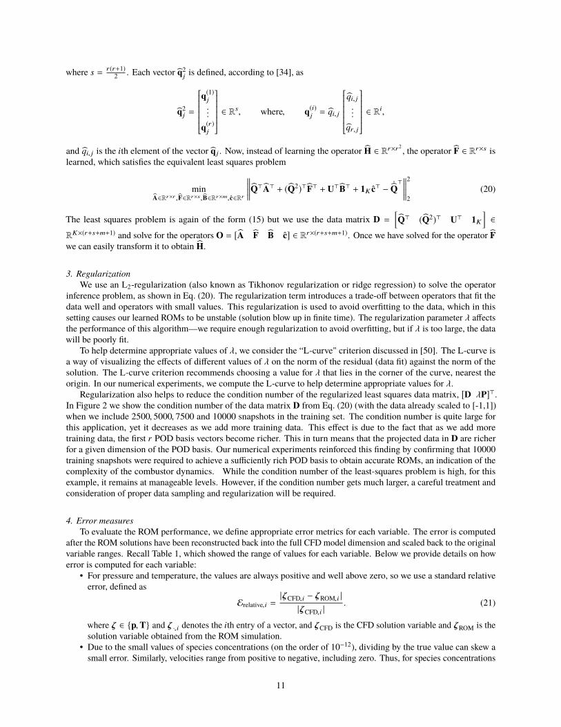
Regularization also helps to reduce the condition number of the regularized least squares data matrix, [D λP]>.In Figure 2 we show the condition number of the data matrix D from Eq. (20) (with the data already scaled to [-1,1])when we include 2500, 5000, 7500 and 10000 snapshots in the training set. The condition number is quite large forthis application, yet it decreases as we add more training data. This effect is due to the fact that as we add moretraining data, the first r POD basis vectors become richer. This in turn means that the projected data in D are richerfor a given dimension of the POD basis. Our numerical experiments reinforced this finding by confirming that 10000training snapshots were required to achieve a sufficiently rich POD basis to obtain accurate ROMs, an indication of thecomplexity of the combustor dynamics. While the condition number of the least-squares problem is high, for thisexample, it remains at manageable levels. However, if the condition number gets much larger, a careful treatment andconsideration of proper data sampling and regularization will be required.

4. Error measuresTo evaluate the ROM performance, we define appropriate error metrics for each variable. The error is computed

after the ROM solutions have been reconstructed back into the full CFD model dimension and scaled back to the originalvariable ranges. Recall Table 1, which showed the range of values for each variable. Below we provide details on howerror is computed for each variable:

• For pressure and temperature, the values are always positive and well above zero, so we use a standard relativeerror, defined as

Erelative,i =|ζCFD,i − ζROM,i ||ζCFD,i |

. (21)

where ζ ∈ {p,T} and ζ ·,i denotes the ith entry of a vector, and ζCFD is the CFD solution variable and ζROM is thesolution variable obtained from the ROM simulation.

• Due to the small values of species concentrations (on the order of 10−12), dividing by the true value can skew asmall error. Similarly, velocities range from positive to negative, including zero. Thus, for species concentrations

11

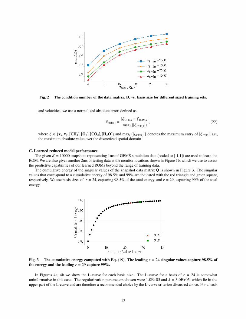
Fig. 2 The condition number of the data matrix, D, vs. basis size for different sized training sets.

and velocities, we use a normalized absolute error, defined as

Enabs,i =|ζCFD,i − ζROM,i |maxl

(|ζCFD,l |

) , (22)

where ζ ∈ {vx, vy, [CH4], [O2], [CO2], [H2O]} and maxl(|ζCFD,l |

)denotes the maximum entry of |ζCFD |, i.e.,

the maximum absolute value over the discretized spatial domain.

C. Learned reduced model performanceThe given K = 10000 snapshots representing 1ms of GEMS simulation data (scaled to [-1,1]) are used to learn the

ROM. We are also given another 2ms of testing data at the monitor locations shown in Figure 1b, which we use to assessthe predictive capabilities of our learned ROMs beyond the range of training data.

The cumulative energy of the singular values of the snapshot data matrix Q is shown in Figure 3. The singularvalues that correspond to a cumulative energy of 98.5% and 99% are indicated with the red triangle and green square,respectively. We use basis sizes of r = 24, capturing 98.5% of the total energy, and r = 29, capturing 99% of the totalenergy.

Fig. 3 The cumulative energy computed with Eq. (19). The leading r = 24 singular values capture 98.5% ofthe energy and the leading r = 29 capture 99%.

In Figures 4a, 4b we show the L-curve for each basis size. The L-curve for a basis of r = 24 is somewhatuninformative in this case. The regularization parameters chosen were 1.0E+05 and λ = 3.0E+05, which lie in theupper part of the L-curve and are therefore a recommended choice by the L-curve criterion discussed above. For a basis

12

(a) Basis size r = 24. (b) Basis size r = 29.

Fig. 4 The L-curve for different basis sizes and regularization parameters λ. The horizontal axis shows thesquared norm of learned operators, ‖O‖22 , and the vertical axis shows the least squares residual, ‖DO> − ÛQ

>‖22 .

of size of r = 29, the L-curve indicates a regularization parameter around λ = 3.0E+04. Stable systems are producedfor λ = 3.0E+04 and 5.0E+04.

We simulate the learned ROM for the two model sizes r = 24 and r = 29 with the same initial value and time stepsize (∆t = 1 × 10−7s) as those used to generate the training set. Since the ROM was constructed from data scaled to[-1,1], we solve the ROM in the (scaled) subspace, and then reconstruct the dimensional quantities by reversing thescaling. Figures 5 and 6 compare the time trace of pressure computed by GEMS (our “truth” data) with the ROMpredictions for 30000 time steps (10000 time steps used for training, 20000 time steps are pure prediction for the ROM)at the cell located at (0.0, 0.0225) in the domain (denoted as monitor location 1 in Figure 1b). The performance of theROM on the training data (first 1ms of data) is good in both cases, although the r = 29 ROM (Figure 6) is more accurate.For test data predictions beyond the training data, both ROMs yield accurate phase predictions and pressure oscillationamplitudes that are good approximations of the truth.

(a) λ = 1.0E + 05. (b) λ = 3.0E + 05.

Fig. 5 Pressure time traces for basis size r = 24. Training with 10000 snapshots. Black vertical line denotesthe end of the training data and the beginning of the test data.

A Galerkin-projection-based POD method was applied to this GEMS model in Ref. [11]. The authors there foundthat a large number of modes (r > 100) was necessary to obtain stable ROMs. Moreover, comparable accuracy,e.g., for the pressure probe predictions shown here, was only achieved with r = 200 POD modes for the ROM (c.f.Fig. 15 in Ref. [11] with Figures 5–6 herein; both are recording pressure at the same probe location). Consequently,while our learned ROM does not resolve the full flow physics, we do obtain good predictability in time at much lowerROM dimension than in the classical Galerkin-POD approach used in Ref. [11]. The key innovation leading to this

13

(a) λ = 3.0E + 04. (b) λ = 5.0E + 04.

Fig. 6 Pressure time traces for basis size of r = 29. Training with 10000 snapshots. Black vertical line denotesthe end of the training data and the beginning of the test data.

improvement is our use of variable transformations to build the ROM over a space for which the transformed governingequations have more polynomial structure. The non-intrusive operator inference approach is an enabler that makes thesevariable transformations practical from an implementation perspective, since the transformations are applied only to thesnapshot data and not to the CFD model itself.

We also compute the average error of each variable over the entire domain at the last time step of the training set(the 10000th time step). The normalized absolute error, defined in Eq. (22), is shown for each species and for x and y

velocity in Figure 7. This figure also shows the relative error, defined in Eq. (21), for pressure and temperature. Theseplots show that overall, the error is decreasing with an increasing basis size. At a basis size of 18, 22, and 24 the systemswere unstable (solution blow up in finite time) and so these basis sizes are excluded from the figure. The cause ofthis, and the non-monotone error decay, may be due to the fact that the same regularization parameter was used foreach of these, λ = 3.0E+04. Ideally, one would pick a parameter specific for the basis size, but here we used the sameregularization parameter in order to give a fairer assessment of the ROM performance without using manual tuningto optimize our results. We note, however, that even with manual tuning of the regularization parameters we are notguaranteed monotone state-error decay for strongly nonlinear dynamical system ROMs.

Fig. 7 Error measures vs. basis size, averaged over the spatial domain at the last time step of training data.Normalized absolute error (22) of species CH4,O2,CO2,H2O and vx and vy velocities; Relative error (21) givenfor pressure and temperature.

In Figure 8, we show the integrated species concentrations over time. To compute these, at each time step in oursimulation, we sum all elements of a species vector. This measure monitors whether our ROM conserves species mass,an important feature of a physically meaningful simulation. As the discretization of the high-fidelity model becomesfiner, point-wise error may become large and misleading if the mass is shifted slightly into the neighboring cells. The

14

integrated species concentration complements the evaluation of point-wise errors and provides a global view of the errorin the domain. While CH4 conservation is tracked well qualitatively by the ROM, it does show the largest deviationout of the four species. This is a result of CH4 having the sharpest gradients (CH4 concentration ranging from 0 to 1)compared to the other three species, see also Figures 13–16 below, and their respective color bars.

Fig. 8 Integrated species at each time step for different basis sizes. Training with 10000 snapshots.

We also compare the state variables over the entire domain predicted by the learned ROM with the given GEMS dataat the last time step K = 10000 (which corresponds to t = 0.0159999s). We provide the true field, the ROM-predictedfield, and an error field for each variable in Figures 9–16. Again, for pressure and temperature, we use a relative errorfrom Eq. (21). For x and y velocity and for species molar concentrations we use a normalized absolute error fromEq. (22). The plots show that the ROM predictions are, as expected, not perfect, but indeed they capture well the overallstructure and many details of the solution fields.

(a) True pressure. (b) Relative error of pressure.

(c) Predicted pressure.

Fig. 9 Predictive results for pressure at the last time step of training data. Training with 10000 snapshots, abasis size of r = 29, and regularization set to λ = 3.0E + 04.

Table 2 shows timing results for the ROM generation and simulation, as performed using python 3.6.4 on a dual-coreIntel i5 processor with 2.3 GHz and 16GB RAM.We report the following CPU times: solving the operator inference leastsquares problem (20); ROM runtime for the two different basis sizes for 3ms of real time prediction; and reconstructionof the high-dimensional, unscaled combustion variables. The latter is required since the ROM is evolving the dynamicsin the [−1, 1] scaled variables, and thus a post-processing step is required to obtain the true magnitudes of the variables.

15

(a) True velocity vx . (b) Normalized absolute error of velocity vx .

(c) ROM-predicted velocity vx .

Fig. 10 Predictive results for velocity vx at the last time step of training data. Training with 10000 snapshots,a basis size of r = 29, and regularization set to λ = 3.0E + 04.

(a) True velocity vy . (b) Normalized absolute error of velocity vy .

(c) ROM-predicted velocity vy .

Fig. 11 Predictive results for velocity vy at the last time step of training data. Training with 10000 snapshots,a basis size of r = 29, and regularization set to λ = 3.0E + 04.

In comparison with the approximately 200h of CPU time needed on a 40-core architecture (more details in Section IV.A)to compute the first 10000 snapshots of data, the ROMs provide five to six orders of magnitude in computationalspeedup.

Table 2 CPU times for two ROMs with time step size ∆t = 1 × 10−7s and 30000 time steps.

ROM order LS solve of (16) ROM simulation Reconstructing high-dim. fieldr = 24 2.80s 6.06s 0.04sr = 29 6.05s 6.22s 0.05s

16

(a) True temperature. (b) Relative error of temperature.

(c) Predicted temperature.

Fig. 12 Predictive results for temperature at the last time step of training data. Training with 10000 snapshots,a basis size of r = 29, and regularization set to λ = 3.0E + 04.

(a) True CH4. (b) Normalized absolute error of CH4.

(c) Predicted CH4.

Fig. 13 Predictive results for CH4 molar concentration at the last time step of training data. Training with10000 snapshots, a basis size of r = 29, and regularization set to λ = 3.0E + 04.

(a) True O2. (b) Normalized absolute error of O2.

(c) Predicted O2.

Fig. 14 Predictive results for O2 molar concentration at the last time step of training data. Training with10000 snapshots, a basis size of r = 29, and regularization set to λ = 3.0E + 04.

17

(a) True CO2. (b) Normalized absolute error of CO2.

(c) Predicted CO2.

Fig. 15 Predictive results for CO2 molar concentration at the last time step of training data. Training with10000 snapshots, a basis size of r = 29, and regularization set to λ = 3.0E + 04.

(a) True H2O. (b) Normalized absolute error of H2O.

(c) Predicted H2O.

Fig. 16 Predictive results for H2O molar concentration at the last time step of training data. Training with10000 snapshots, a basis size of r = 29, and regularization set to λ = 3.0E + 04.

18

V. ConclusionOperator inference is a data-driven method for learning reduced-order models (ROMs) of dynamical systems with

polynomial structure. This paper demonstrates how variable transformations can expose quadratic structure in thenonlinear system of partial differential equations describing a complex combustion model. This quadratic structureis preserved under projection, providing the mathematical justification for learning a quadratic ROM using operatorinference. An important feature of the approach is that the learning of the ROM is non-intrusive—it requires statesolutions generated by running the high-fidelity combustion model, but it does not require access to the discretizedoperators of the governing equations. This is important because it means that the variable transformations can be appliedas a post-processing step to the simulation data set, but no intrusive modifications are needed to the high-fidelity code.While the quadratic model form is an approximation for this particular application problem, the numerical results showthat the learned quadratic ROM can predict relevant quantities of interest and can also conserve species accurately. Manynonlinear equations in scientific and engineering applications admit variable transformations that expose polynomialstructure. This combined with the non-intrusive nature of the approach make it a viable option for deriving ROMs forcomplex nonlinear applications where traditional intrusive model reduction is impractical and/or unreliable. Whilewe improved ROM stability through the presented regularization of the least-squares problem, some of the ROMswere unstable. Future work thus includes devising alternative approaches (see e.g., [23, 24]) and developing theory toguarantee stable learned ROMs.

Appendix A: Lifting chemical source termsThe chemical source terms in ®S in Eq. (4) are Ûωl = Ml Ûcreactionl

, see Eq. (6). The dynamics for the source termsÛcreactionl

are given by

Ûcreaction1 = −A exp(− Ea

RuT

)c0.2

1 c1.32 , (23a)

Ûcreaction2 = 2 Ûcreaction1 , (23b)Ûcreaction3 = − Ûcreaction1 , (23c)Ûcreaction4 = −2 Ûcreaction1 . (23d)

To lift this system to polynomial form, we introduce the auxiliary variables

w1 = c0.21 , w2 = c−1

1 , w3 = c1.32 , w4 = c−1

2 , w5 = exp(− Ea

RuT

), w6 =

1T2 .

The source term dynamics (23) are then cubic in w1,w3,w5:

Ûcreaction1 = −Aw1w3w5, (24a)Ûcreaction2 = 2Aw1w3w5, (24b)Ûcreaction3 = −Aw1w3w5, (24c)Ûcreaction4 = −2Aw1w3w5. (24d)

We next derive the dynamics for the auxiliary variablesw1, . . . ,w6. For instance, we have Ûw1 = 0.2c0.2−11 Ûc1 = 0.2w1w2 Ûc1.

Similarly, we obtain the system of auxiliary dynamics:

Ûw1 = 0.2w1w2 Ûc1, Ûw2 = −w21 Ûc1,

Ûw3 = 1.3w3w4 Ûc2, Ûw4 = −w24 Ûc2,

Ûw5 =Ea

Ru

1T2 w5 ÛT =

Ea

Ruw5w6 ÛT, Ûw6 = −2

1T3 = −2Tw2

6 .

19

The dynamics of the lifted variables are quintic in the variables w1, . . . ,w6. If we further include an additional auxiliaryvariable w7 = w1w3w5, then we obtain the system of equations

Ûw1 = 0.2Aw1w2w7, Ûw2 = −Aw21w7,

Ûw3 = 2.6Aw3w4w7, Ûw4 = −2Aw24w7,

Ûw5 =Ea

Ruw5w6 ÛT, Ûw6 = −2Tw2

6,

0 = w7 − w1w3w5.

The temperature T = pξR(Yl ) can be obtained from the states ξ, p,Yl via the ideal gas relationship in Eq. (8).

Appendix B: Equations for pressure and chemical speciesHere, we give the complete governing equation for the species molar concentrations cl and pressure p. Recall from

Section III.C the notation used to denote the conservative variables gi: g1 = ρ, g2 = ρvx, g3 = ρvy, g4 = ρe, g5 =ρY1, g6 = ρY2, g7 = ρY3, g8 = ρY4.

Species molar concentrations cl: For the species molar concentration dynamics, we use the relationship cl =ρYlMl

fromEq. (5), where the constants M1, . . . , M4 are molar masses. We obtain for l = 1, 2, . . . , nsp:

∂cl∂t=

1Ml

∂ρYl∂t

=1

Ml

(Ûωl + ∇ ·

(−vxρYl®i − vyρYl ®j + ®jml

))=

1Ml

(Ml Ûcreactionl − Ml

(∂vxcl∂x

+∂vycl∂y

)+ ∇ · ®jml

)= Ûcreactionl −

(∂vxcl∂x

+∂vycl∂y

+1

Ml∇ · ®jml

).

Note that the chemical source terms Ûcreactionl

were given in Appendix A, and from Eq. (24) we see that the Ûcl are cubic inthe auxiliary lifted states w1, . . . ,w6. The divergence term is

∇ · ®jml = Dl

(∂

∂x

(ρ∂Yl∂x

)+

∂

∂y

(ρ∂Yl∂y

)),

and since Yl = Mlclξ, we have that

ρ∂Yl∂x= ρMl

∂clξ∂x= Ml

(∂cl∂x+ ρcl

∂ξ

∂x

).

Overall, we have that

∂cl∂t= Ûcreactionl −

(∂vxcl∂x

+∂vycl∂y

+∂cl∂x+ ρcl

∂ξ

∂x+∂cl∂y+ ρcl

∂ξ

∂y

),

which is quadratic in the learning variables vx, vy, cl with the exception of the terms ρcl∂ξ∂x and ρcl

∂ξ∂y . We note that if ρ

were included as a lifted variable (in addition to ξ), these terms would become quadratic in the lifted state.

Pressure p: We start with the energy equation (2). By multiplying with density ρ, we have ρe = ρh0 − p, so from theconservation equation (1) for ρe we obtain

∂(ρh0 − p)∂t

+∂ρvxh0

∂x+∂ρvyh0

∂y+

∂

∂x(vxτxx + vyτyx − jqx ) +

∂

∂y(vxτxy + vyτyy − jqy ) = 0.

This directly gives an equation for the time evolution of pressure:

∂p∂t=∂ρh0

∂t+∂ρvxh0

∂x+∂ρvyh0

∂y+

∂

∂x(vxτxx + vyτyx − jqx ) +

∂

∂y(vxτxy + vyτyy − jqy ).

20

Moreover, per definition of h0 in Eq. (2) and with cl =ρYlMl

we have that

∂ρh0

∂t=

nsp∑i=1

∂ρhlYl∂t

+∂ρ 1

2

(v2x + v

2y

)∂t

=

nsp∑i=1

Ml∂hlcl∂t+

12

(v2x + v

2y

) ∂ρ∂t+ ρ

∂(vx + vy)∂t

.

Overall, we have that

∂p∂t=

nsp∑i=1

Ml

(hl∂cl∂t+ cl

∂hl∂t

)+

12

(v2x + v

2y

) ∂ρ∂t+ ρ

∂(vx + vy)∂t

+∂ρvxh0

∂x+∂ρvyh0

∂y

+∂

∂x(vxτxx + vyτyx − jqx ) +

∂

∂y(vxτxy + vyτyy − jqy ).

This equation remains nonlinear in our chosen learning variables ®qL . In particular, the enthalpies hl = hl(T) and theirtime derivatives are nonlinear functions of temperature. The other terms show some polynomial structure; for example,in Section III.C we showed that ∂(vx+vy )∂t is quadratic in the learning state variables p, vx, vy, ξ. However, to write thisequation exactly in a polynomial form would require introducing a large number of auxiliary variables along with theircorresponding dynamics. We have instead chosen to introduce an approximation by learning a ROM in the variables ®qL

with quadratic form.

Funding SourcesThis work has been supported in part by the Air Force Center of Excellence on Multi-Fidelity Modeling of

Rocket Combustor Dynamics award FA9550-17-1-0195, and the Air Force Office of Scientific Research (AFOSR)MURI on managing multiple information sources of multi-physics systems award numbers FA9550-15-1-0038 andFA9550-18-1-0023.

References[1] Bui-Thanh, T., Damodaran, M., and Willcox, K. E., “Aerodynamic data reconstruction and inverse design using proper

orthogonal decomposition,” AIAA Journal, Vol. 42, No. 8, 2004, pp. 1505–1516.

[2] Tadmor, G., Centuori, M., Lehmann, O., Noack, B., Luctenburg, M., and Morzynski, M., “Low Order Galerkin Models for theActuated Flow Around 2-D Airfoils,” 45th AIAA Aerospace Sciences Meeting and Exhibit, 2007, p. 1313.

[3] Lieu, T., and Farhat, C., “Adaptation of Aeroelastic Reduced-Order Models and Application to an F-16 Configuration,” AIAAJournal, Vol. 45, No. 6, 2007, pp. 1244–1257.

[4] Amsallem, D., Cortial, J., and Farhat, C., “Towards Real-Time Computational-Fluid-Dynamics-Based Aeroelastic Computationsusing a Database of Reduced-Order Information,” AIAA Journal, Vol. 48, No. 9, 2010, pp. 2029–2037.

[5] Berger, Z., Low, K., Berry, M., Glauser, M., Kostka, S., Gogineni, S., Cordier, L., and Noack, B., “Reduced Order Models for aHigh Speed Jet with Time-Resolved PIV,” 51st AIAA Aerospace Sciences Meeting including the New Horizons Forum andAerospace Exposition, 2013, p. 11.

[6] Brunton, S. L., Rowley, C. W., andWilliams, D. R., “Reduced-Order Unsteady Aerodynamic Models at Low Reynolds Numbers,”Journal of Fluid Mechanics, Vol. 724, 2013, p. 203–233.

[7] Kramer, B., Grover, P., Boufounos, P., Nabi, S., and Benosman, M., “Sparse Sensing and DMD-Based Identification ofFlow Regimes and Bifurcations in Complex Flows,” SIAM Journal on Applied Dynamical Systems, Vol. 16, No. 2, 2017, pp.1164–1196.

[8] Nguyen, V., Buffoni, M., Willcox, K., and Khoo, B., “Model reduction for reacting flow applications,” International Journal ofComputational Fluid Dynamics, Vol. 28, No. 3-4, 2014, pp. 91–105.

[9] Nguyen, V. B., Dou, H.-S., Willcox, K., and Khoo, B.-C., “Model Order Reduction for Reacting Flows: Laminar GaussianFlame Applications,” 30th International Symposium on Shock Waves 1, Springer, 2017, pp. 337–343.

[10] Buffoni, M., and Willcox, K., “Projection-based model reduction for reacting flows,” 40th Fluid Dynamics Conference andExhibit, Chicago, IL, June 28-July 1, 2010, p. 5008.

21

[11] Huang, C., Duraisamy, K., and Merkle, C. L., “Investigations and Improvement of Robustness of Reduced-Order Models ofReacting Flow,” AIAA Journal, Vol. 0, No. 0, 0, pp. 1–13. doi:10.2514/1.J058392, URL https://doi.org/10.2514/1.J058392.

[12] Huang, C., Xu, J., Duraisamy, K., and Merkle, C., “Exploration of reduced-order models for rocket combustion applications,”2018 AIAA Aerospace Sciences Meeting, 2018, p. 1183.

[13] Wang, Q., Hesthaven, J. S., and Ray, D., “Non-intrusive reduced order modeling of unsteady flows using artificial neuralnetworks with application to a combustion problem,” Journal of computational physics, Vol. 384, 2019, pp. 289–307.

[14] Lumley, J. L., “The Structure of Inhomogeneous Turbulent Flows,” Atmospheric Turbulence and Radio Wave Propagation,1967.

[15] Sirovich, L., “Turbulence and the Dynamics of Coherent Structures. I-Coherent Structures. II-Symmetries and Transformations.III-Dynamics and Scaling,” Quarterly of Applied Mathematics, Vol. 45, 1987, pp. 561–571.

[16] Veroy, K., Rovas, D. V., and Patera, A. T., “A posteriori error estimation for reduced-basis approximation of parametrized ellipticcoercive partial differential equations: ‘convex inverse’ bound conditioners,” ESAIM: Control, Optimisation and Calculus ofVariations, Vol. 8, 2002, pp. 1007–1028.

[17] Grepl, M. A., Maday, Y., Nguyen, N. C., and Patera, A. T., “Efficient Reduced-Basis Treatment of Nonaffine and NonlinearPartial Differential Equations,” ESAIM: Mathematical Modelling and Numerical Analysis, Vol. 41, No. 3, 2007, pp. 575–605.

[18] Tröltzsch, F., and Volkwein, S., “POD a-posteriori error estimates for linear-quadratic optimal control problems,” ComputationalOptimization and Applications, Vol. 44, No. 1, 2009, p. 83.

[19] Hesthaven, J. S., Rozza, G., and Stamm, B., Certified reduced basis methods for parametrized partial differential equations,Springer, 2016.

[20] Rowley, C. W., Colonius, T., and Murray, R. M., “Model reduction for compressible flows using POD and Galerkin projection,”Physica D: Nonlinear Phenomena, Vol. 189, No. 1-2, 2004, pp. 115–129.

[21] Barone, M. F., Kalashnikova, I., Segalman, D. J., and Thornquist, H. K., “Stable Galerkin reduced order models for linearizedcompressible flow,” Journal of Computational Physics, Vol. 228, No. 6, 2009, pp. 1932–1946.

[22] Serre, G., Lafon, P., Gloerfelt, X., and Bailly, C., “Reliable reduced-order models for time-dependent linearized Euler equations,”Journal of Computational Physics, Vol. 231, No. 15, 2012, pp. 5176–5194.

[23] Kalashnikova, I., and Barone, M., “Stable and efficient Galerkin reduced order models for non-linear fluid flow,” 6th AIAATheoretical Fluid Mechanics Conference, 2011, p. 3110.

[24] Balajewicz, M., Tezaur, I., and Dowell, E., “Minimal subspace rotation on the Stiefel manifold for stabilization and enhancementof projection-based reduced order models for the compressible Navier–Stokes equations,” Journal of Computational Physics,Vol. 321, 2016, pp. 224–241.

[25] Carlberg, K., Barone, M., and Antil, H., “Galerkin v. least-squares Petrov–Galerkin projection in nonlinear model reduction,”Journal of Computational Physics, Vol. 330, 2017, pp. 693–734.

[26] Huang, C., Duraisamy, K., and Merkle, C., “Challenges in Reduced Order Modeling of Reacting Flows,” 2018 Joint PropulsionConference, 2018, p. 4675.

[27] Hornik, K., Stinchcombe, M., and White, H., “Multilayer feedforward networks are universal approximators,” Neural networks,Vol. 2, No. 5, 1989, pp. 359–366.

[28] Swischuk, R., Mainini, L., Peherstorfer, B., and Willcox, K., “Projection-based model reduction: formulations for physics-basedmachine learning,” Computers and Fluids, Vol. 179, 2019, pp. 704–717.

[29] Brunton, S. L., Proctor, J. L., and Kutz, J. N., “Discovering governing equations from data by sparse identification of nonlineardynamical systems,” Vol. 113, No. 15, 2016, pp. 3932–3937. doi:10.1073/pnas.1517384113.

[30] Rudy, S. H., Brunton, S. L., Proctor, J. L., and Kutz, J. N., “Data-driven discovery of partial differential equations,” ScienceAdvances, Vol. 3, No. 4, 2017, p. e1602614.

[31] Schaeffer, H., Tran, G., and Ward, R., “Extracting sparse dynamics from limited data,” SIAM Journal on Applied Mathematics,Vol. 78, No. 6, 2018, pp. 3279–3295.

22

[32] Schmid, P. J., “Dynamic mode decomposition of numerical and experimental data,” Journal of Fluid Mechanics, Vol. 656,2010, pp. 5–28.

[33] Rowley, C. W., Mezić, I., Bagheri, S., Schlatter, P., and Henningson, D. S., “Spectral analysis of nonlinear flows,” Journal ofFluid Mechanics, Vol. 641, 2009, pp. 115–127.

[34] Peherstorfer, B., and Willcox, K., “Data-driven operator inference for nonintrusive projection-based model reduction,” ComputerMethods in Applied Mechanics and Engineering, Vol. 306, 2016, pp. 196–215.

[35] Qian, E., Kramer, B., Marques, A., andWillcox, K., “Transform & Learn: A data-driven approach to nonlinear model reduction,”AIAA Aviation and Aeronautics Forum and Exposition, Dallas, TX, 2019. doi:10.2514/6.2019-3707.

[36] Gu, C., “QLMOR: A projection-based nonlinear model order reduction approach using quadratic-linear representation ofnonlinear systems,” IEEE Transactions on Computer-Aided Design of Integrated Circuits and Systems, Vol. 30, No. 9, 2011, pp.1307–1320.

[37] Kramer, B., and Willcox, K., “Nonlinear Model Order Reduction via Lifting Transformations and Proper OrthogonalDecomposition,” AIAA Journal, Vol. 57, No. 6, 2019, pp. 2297–2307. doi:10.2514/1.J057791.

[38] Kramer, B., and Willcox, K., “Balanced Truncation Model Reduction for Lifted Nonlinear Systems,” Tech. rep., 2019.ArXiv:1907.12084.

[39] Harvazinski, M. E., Huang, C., Sankaran, V., Feldman, T. W., Anderson, W. E., Merkle, C. L., and Talley, D. G., “Couplingbetween hydrodynamics, acoustics, and heat release in a self-excited unstable combustor,” Physics of Fluids, Vol. 27, No. 4,2015, p. 045102.

[40] Harvazinski, M. E., “Modeling self-excited combustion instabilities using a combination of two-and three-dimensionalsimulations,” Ph.D. thesis, Purdue University, 2012.

[41] Huang, C., Gejji, R., Anderson, W., Yoon, C., and Sankaran, V., “Combustion Dynamics in a Single-Element Lean DirectInjection Gas Turbine Combustor,” Combustion Science and Technology, 2019, pp. 1–28.

[42] Yu, Y., O’Hara, L., Sisco, J., and Anderson, W., “Experimental study of high-frequency combustion instability in a continuouslyvariable resonance combustor (CVRC),” 47th AIAA Aerospace Sciences Meeting, Orlando, FL, 2009.

[43] Westbrook, C. K., and Dryer, F. L., “Simplified reaction mechanisms for the oxidation of hydrocarbon fuels in flames,”Combustion Science and Technology, Vol. 27, No. 1-2, 1981, pp. 31–43.

[44] Martins, J. R., andHwang, J. T., “Review and unification ofmethods for computing derivatives of multidisciplinary computationalmodels,” AIAA journal, Vol. 51, No. 11, 2013, pp. 2582–2599.

[45] Knowles, I., and Renka, R. J., “Methods for numerical differentiation of noisy data,” Electron. J. Differ. Equ, Vol. 21, 2014, pp.235–246.

[46] Chartrand, R., “Numerical differentiation of noisy, nonsmooth, multidimensional data,” 2017 IEEE Global Conference onSignal and Information Processing (GlobalSIP), IEEE, 2017, pp. 244–248.

[47] Golub, G. H., and Van Loan, C. F., “Matrix computations. 1996,” Johns Hopkins University, Press, Baltimore, MD, USA, 1996,pp. 374–426.

[48] Swischuk, R. C., “Physics-based machine learning and data-driven reduced-order modeling,” Master’s thesis, MassachusettsInstitute of Technology, 2019.

[49] Martinsson, P.-G., Rokhlin, V., and Tygert, M., “A randomized algorithm for the decomposition of matrices,” Applied andComputational Harmonic Analysis, Vol. 30, No. 1, 2011, pp. 47–68.

[50] Hansen, P., “The L-curve and its use in the numerical treatment of inverse problems,” Computational Inverse Problems inElectrocardiology, Vol. 5, 2001, pp. 119–142.

23