least absolute deviations estimation for the censored

Journal of Econometrics 25 (1984) 303-325. North-Holland

LEAST ABSOLUTE DEVIATIONS ESTIMATION FOR THE CENSORED REGRESSION MODEL*

James L. POWELL

Massachusetts Institute of Technology, Cambridge, MA 02 I39, USA

Received May 1983, final version received October 1983

This paper proposes an alternative to maximum likelihood estimation of the parameters of the censored regression (or censored ‘Tobit’) model. The proposed estimator is a generalization of least absolute deviations estimation for the standard linear model, and, unlike estimation methods based on the assumption of normally distributed error terms, the estimator is consistent and asymptotically normal for a wide class of error distributions, and is also robust to heteroscedasticity. The paper gives the regularity conditions and proofs of these large-sample results, and proposes classes of consistent estimators of the asymptotic covariance matrix for both homoscedastic and heteroscedastic disturbances.

1. Introduction

Many of the important recent advances in econometric methods pertain to limited dependent variable models - that is, regression models for which the range of the dependent variable is restricted to some subset of the real line. Such prior restrictions quite commonly arise in cross-section studies of economic behavior; often, for some fraction of individuals in a sample, implicit non-negativity or other inequality constraints are binding for the variable of interest. In a regression model, an inequality constraint for the dependent variable results in a corresponding bound on the unobservable error terms, this bound being systematically related to the value of the regression function. Hence, the mean of the restricted error term is not zero, and the usual conditions for consistency of least squares estimation will not apply.

The regression model with a non-negativity constraint on the dependent variable was proposed by Tobin (1958); consistent estimation of the parameters of the regression function has been investigated by Amemiya (1973) and Heckman (1976,1979). Amemiya demonstrates the consistency and asymptotic normality of maximum likelihood estimation for this model, termed the

*This research was supported by National Science Foundation Grants SES79-12965 and SES79-13976 at the Institute for Mathematical Studies in the Social Sciences at Stanford Univer- sity. I would like to thank Takeshi Amemiya, Theodore W. Anderson, Timothy Bresnahan, Cohn Cameron, Jerry Hausman, Thomas MaCurdy, Daniel McFadden, Julio Rotemberg, and the referees for their helpful comments.

0304-4076/84/$3.00~1984, Elsevier Science Publishers B.V. (North-Holland)

304 J. L. Powell, LAD estimation for regression models

censored regression or censored ‘Tobit’ model, while Heckman extends least squares estimation to a more general limited dependent variable model by expressing the conditional expectation of the dependent variable as a known (nonlinear) function of the regressors and unknown parameters. A feature common to these approaches is the assumption that the error terms are normally distributed. This condition is essential to the proofs of consistency; unlike the standard linear regression model, for which normal maximum likelihood estimation (classical least squares) is consistent for a wide class of distributions of the residual, estimators based on normality in limited dependent variable models are inconsistent when the normality assumption is violated. Goldberger (1980) and Arabmazar and Schmidt (1982) illustrate this point by calculating the inconsistency of the normal maximum likelihood estimator for several common non-normal distributions of the error term.

This study extends least absolute deviations (LAD) estimation to the regression model with non-negativity of the dependent variable, and gives conditions under which this estimator is consistent and asymptotically normal. In view of the sensitivity of maximum likelihood and least squares methods to the assumption of normality in this model, it is somewhat surprising that a simple modification of LAD estimation yields a consistent estimator which does not depend upon the functional form of the distribution of the residuals.’ In this sense the estimator proposed below is non-parametric, although its consistency and asymptotic normality require stronger assumptions on the behavior of the regression function than those imposed on models with normal residuals. As for the standard regression model, LAD estimation may be computationally burdensome for the censored regression model, because the function to be minimized is not continuously differentiable; nevertheless, it does provide a consistent alternative to likelihood-based procedures when prior information on the parametric form of the error density is unavailable.

In the next section, the censored regression model and the corresponding LAD estimator are defined; the sections which follow give the appropriate regularity conditions for (strong) consistency and asymptotic normality of the estimator. Section 5 shows how consistent estimators of the asymptotic covari- ante matrix of the estimator can be obtained. The final section summarizes the foregoing results, and points out some unresolved issues as topics for further research.

‘Other non-parametric estimators of the parameters of the censored regression model have been proposed by Buckley and James (1979) and Kalbfleisch and Prentice (1980, ch. 6). The former study combines estimation based upon the ‘EM algorithm’ [see Dempster, Laird, and Rubin (1977)] with the Kaplan-Meier (1958) non-parametric estimator of the survival curve, while the latter is based upon rank regression techniques. It is asserted (though not rigorously demonstrated) that these estimators are also consistent and asymptotically normal. Whether they are to be preferred to the estimator proposed here, on computational or efficiency grounds, is an open question; however, unlike the censored LAD estimator, they are apparently not robust to heteroscedasticity of the error terms.

J.L.. Powell, LAD estimation for regression models 305

2. Definitions and motivation

The censored regression model considered below can be written in the form

yt = max{ 0, $PO + u, }, t=l,...,T, (2.1)

where the dependent variable y, and regression vector x, are observed for each t, while the (conformable) parameter vector & and error term u, are unob- served. It will be presumed throughout that estimation of &, is the primary object of the statistical analysis (as opposed to, say, estimation of the conditional probability that yr exceeds zero given xt).

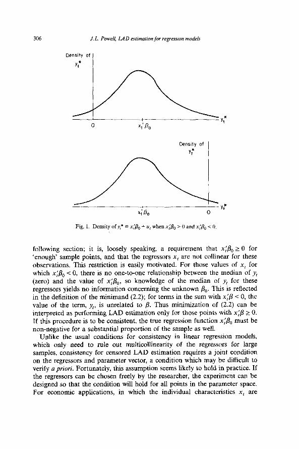
The definition of the LAD estimator for this model will be based on the fact that, for any scalar random variable Z, the function E[]Z- b] - ]Z]] is minimized by choosing b to be a median of the distribution of Z. Hence, if the median of y, is some known function m(x,, &) of the regressors and unknown parameters, a sample analogue to the conditional median can be defined by choosing fir so that the function (l/T)& - m(x,, p)I is minimized at the value /I = &. But suppose the error term u, is continuously distributed with median zero, and that the density function is positive at zero (so that the median of u, is unique). Then it is easy to verify that the median function for yI takes a particularly simple form, namely, m(x,, &,) = max{O, x;& }. This fact is illustrated in fig. 1. In the top panel, for which xl& > 0, the probability that y, = 0, equivalent to the probability that_@ s xl/l0 + u, I 0, is less than one-half, and the median of yI is x;&. On the other hand, if xi&, < 0 (the bottom panel of fig. l), the probability that y, equals zero exceeds one-half, and zero is the unique median of y,.

Thus, the LAD estimator for the censored regression model minimizes the sum of absolute deviations of y, from max{O, x;&} over all /3 in the parameter space (denoted B). Algebraically, the censored LAD estimator & minimizes

s,(p)-(I,T)~~~~y,-man(0,x:Pj/ (24

over all p in B.

This minimum will always exist if the parameter space B is compact, since the function S,(p) is continuous. Unfortunately, this minimization may not yield a unique value for &. As a simple example, suppose the sample has y, = 0 for all t. In this case, any value of /3 in B which has x$? I 0 for all t will yield the same minimizing value of S,(p), zero. Of course, this case can be ruled out for large samples, as long as the probability that u, > -x;&, is positive for a substantial proportion of the regressors { xt }; nonetheless, it will be necessary to restrict the possible behavior of the regression function x$, to ensure the uniqueness of the censored LAD estimator &- for large samples. The precise condition to be imposed is given by Assumption R.l of the

J.Econ- C

306 J. L. Powell, IA D estimation for regression models

Density of

y:

Density of

y ;

following section; it is, loosely speaking, a requirement that xi&, 2 0 for ‘enough’ sample points, and that the regressors x, are not collinear for these observations. This restriction is easily motivated. For those values of x, for which x$, < 0, there is no one-to-one relationship between the median of yt (zero) and the value of x;&,, so knowledge of the median of y, for these regressors yields no information concerning the unknown &. This is reflected in the definition of the minimand (2.2); for terms in the sum with ~$3 -C 0, the value of the term, y,, is unrelated to p. Thus minimization of (2.2) can be interpreted as performing LAD estimation only for those points with x$ L 0. If this procedure is to be consistent, the true regression function ni&, must be non-negative for a substantial proportion of the sample as well.

Unlike the usual conditions for consistency in linear regression models, which only need to rule out multicollinearity of the regressors for large samples, consistency for censored LAD estimation requires a joint condition on the regressors and parameter vector, a condition which may be difficult to verify a priori. Fortunately, this assumption seems likely to hold in practice. If the regressors can be chosen freely by the researcher, the experiment can be designed so that the condition will hold for all points in the parameter space. For economic applications, in which the individual characteristics x, are

J. L. Powell, LAD esfima$on for regression models 307

generally not under the control of the researcher, the condition amounts to the assumption that the ‘typical’ (i.e., median) value of the ‘true’ dependent variable yf” = x,‘&, + U, is non-negative for a positive fraction of individuals in the sample, which is not unreasonable for many populations sampled.

The assumptions on the distribution of the error term U, required for consistency are much weaker than those for maximum likelihood or least squares estimators for the censored regression model. It is the fact that the median of the censored variable yt does not depend upon the functional rorm of the density of the errors that makes censored LAD a ‘distribution-free’ estimator, a property not shared by the mean (if it exists) of y,. Hence least absolute deviations estimation is a natural approach for censored data when the assumption of normality of the errors is suspect.

3. Strong consistency of the censored LAD estimator

To show the large-sample (almost sure) convergence of & to the true value &, the following conditions on &, u,, and x, are imposed:

Assumption P. I. The parameter vector & is an element of a compact parameter space B.

Assumption E.1. The error terms { uI} are independently and identically distributed random variables, are independent of the regressors, and have median zero, and the distribution function of U, is continuously differentiable with density which is bounded above and positive at zero. Hence, defining F(F(A)=Pr(u,<h), F(O)=+ and dF(F(X)=f(A)dh withf(A)<f,, somef,>O, and f(0) > 0.

Assumption R.l. The regressors {x,} are independently distributed random vectors with E(IxJ3 < K, for all t and some positive K,, and JJ~, the smallest characteristic root of the matrix

has vT > v0 whenever T > TO, some positive E,,, vO, and TO.2

A few remarks concerning the necessity and generality of these assumptions (beyond those made in the previous section) are in order. The compactness of B would be difficult to relax in this context, since it ensures the existence and

‘The symbol ‘l(A)’ denotes the indicator function of the event ‘A’, i.e., it is a function which takes the value one if A is true and is zero otherwise.


measurability of 8, [by Lemma 2 of Jennrich (1969)] and the uniformity of the (almost sure) convergence of the minimand over B, as required by Lemma A.2 of appendix 1 below.

As usual, the requirement that the errors have median zero is not restrictive, provided there is an unknown constant term in the regression function (although the condition on the matrix in Assumption R.l presumes that the regression function is written so that u, has zero median). Also, the conditions that the error terms are continuously and identically distributed are made for convenience, and can easily be relaxed. It suffices that the conditional distribution of U, given x1 has median zero for all 1, and the corresponding distribution functions for the { ut} only need to be continuously differentiable in a uniform neighborhood of zero, with density functions { f,(X]x,)} which are uniformly bounded away from zero, i.e.,

(3.1)

whenever ]h( < k, some k > 0, all t.

Thus, while Assumption E.l presumes homoscedasticity of the residuals, this condition is not needed for strong consistency of &. (nor for its asymptotic normality, as discussed below), since the conditional median of the dependent variable will still be of the form max{O, x:& }_ This robustness of the censored LAD estimator to (bounded) heteroscedasticity makes it attractive even when the error terms are Gaussian; as Maddala and Nelson (1974) and Arabmazar and Schmidt (1981) have shown, heteroscedastic errors also cause inconsistency of likelihood-based estimators for Tobit models.

Finally, the assumption that the regression vectors { xt} are stochastic and mutually independent is imposed to simplify the additional condition to be imposed below to obtain asymptotic normality of &.; however, since the { xr }

are not presumed to be identically distributed, this assumption is not as restrictive as it might first appear. In particular, this setup will accomodate a fixed design matrix, where the {x, } take fixed (and uniformly bounded) values with probability one. Nevertheless, there may be samples for which the assumption of independence of the { xt } over t is inappropriate (e.g., in panel studies, where the regressors represent several measurements of individual characteristics over time); while independence of the regressors does not appear to be essential to the large-sample results given below, relaxation of this assumption would greatly complicate the discussion of asymptotic normality, and thus will not be pursued here.3

3Robinson (1982) has recently shown Tobit maximum likelihood estimation to be strongly consistent and asymptotically normal under weaker conditions on the dependence of the error terms, and it seems likely that his approach could be extended to the estimator considered here.

J. L. Powell, LAD estimation for regression models 309

Theorem I. For the censored regression model (2.1) under Assumptions P.1, R.l, and El, the censored LAD estimator & is strongly consistent; that is, if

where S,( /3) is defined in (2.2) above, then &- converges to /I,, almost surely.

The proof of this result, as well as the proofs for Theorems 2 and 3 below, are given in appendix 2.

4. Asymptotic normality of the censored LAD estimator

Having established the consistency of the censored LAD estimator &, determination of its asymptotic distribution is the next logical step in the analysis of its sampling properties. However, for estimation methods based upon minimization of an absolute value criterion, distribution theory is complicated by the lack of differentiability of the minimand. Hence the standard approach to the demonstration of asymptotic normality, based on a Taylor’s series expansion of the objective function, is not directly applicable in the present context. Several methods have been used to obtain the large-sample distributions of LAD estimators for the standard linear regression model. Bassett and Koenker (1978) prove the asymptotic normality of LAD in its alternative representation as the solution of a linear programming problem, an approach suggested by Taylor (1974); unfortunately, their proof would be difficult to generalize in the present context, since the minimization problem which defines & cannot be rewritten as a linear program, except possibly in a neighborhood of B r..4 An alternative proof of the limiting normality of standardized LAD regression coefficients has been given by Amemiya (1982), who approximates the sum of absolute deviations by a twice-differentiable function that tends to the same limit function; the LAD estimator is then shown to have the same large-sample behavior as the estimator that minimizes this differentiable function. While this method appears to be more applicable in this case, it is algebraically quite complicated, and thus is not adopted here.

The proofs of asymptotic normality given below are based on an approach used by Huber (1967), Bickel (1975), JureckovB (1977), Ruppert and Carroll (1980), Koenker and Bassett (1982a), and Powell (1983). The proof of asymptotic normality given in appendix 2 uses a simple modification of Huber’s version of this technique, the modification being required because Huber’s

4Minimization of S,(p) cannot be restated as a linear programming problem because the minimand, while piecewise linear, is not convex in 8. However, if at the respective solution values there are no data points for which x$,= 0, then for small variations about fiT the function S,(& will behave just like a sum of absolute deviations for those data points with x$, z 0.

310 .I. L. Powell, LAD estimation for regression models

discussion involves identically distributed random variables. The formal statement of this theorem, along with the conditions for its validity, are given in appendix 1 (Lemma A.3). In short, the lemma approximates the (discontinu- ous) subgradient of the objective function by its continuously differentiable expectation, and then relates this approximation to the asymptotic ‘first-order condition’ defining the estimator (which sets the subgradient equal to zero asymptotically).

For this method to be applicable to the censored LAD estimator, additional regularity conditions are required; that is, conditions P.l, E.l, and R.l are not sufficient in general to ensure that fl( &. - &,) has a limiting normal distribution. One additional condition is needed because the conditional median function max{O, xl/3 } of y, is not well-behaved for values of x, which are nearly orthogonal to p, since the function is not differentiable in p when x$ = 0. To ensure asymptotic normality of &, sequences of values of x, which are orthogonal to & with positive frequency must be ruled out. For this purpose, the following condition will suffice:

Assumption R.2. In addition to the conditions of Assumption R.l, defining

Gt(z, P> r) = E[l( WI 5 llxtll ~z)llxtllr] 7

the function G, is o(z) for z near zero, 0 near &, and r = 0, 1,2, uniformly in t, i.e.,

for some positive K, and [a.

To interpret this condition, first suppose for simplicity that the regressors have bounded support (i.e., lIx,JJ I K with probability one for all t and some K > 0). Then it suffices that Pr( 1x$1 I z) = o(z) uniformly in t for p near & and z near zero, since Pr(lx$l< JJx,JJ . z ) IS no greater than Pr( /x$1 I K - z) in this case. When the { xr } are preassigned vectors, this condition would require that lx~&l> k (with probability one) for some k > 0; for many applications, though, such an assumption would be too restrictive, and this is the reason for the more general condition R.2. Heuristically, the assumption implies that the regression function x$ is distributed much like the corresponding error term u,, at least for /3 near &, and x$ near the censoring point (zero). Obviously, this condition does not exclude deterministic components of the vector x,, nor components which have discrete distributions; only the linear combination x:fi must have a Lipschitz continuous distribution function near zero.

For regressors with unbounded support, it is the ‘normalized’ regression function IIx,II-~x$ which must be smoothly distributed near zero. In addition,

J.L.. Powell, LAD estimufion/or regression models 311

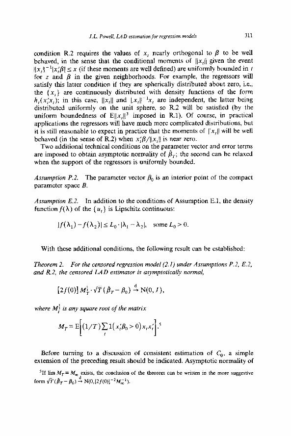
condition R.2 requires the values of x, nearly orthogonal to p to be well behaved, in the sense that the conditional moments of /lx,jJ given the event (Ix,II-~Ix# I x (if these moments are well defined) are uniformly bounded in t for z and /3 in the given neighborhoods. For example, the regressors will satisfy this latter condition if they are spherically distributed about zero, i.e., the { xt} are continuously distributed with density functions of the form h,(xjx,); in this case, llxJ/ and Ijx,ll- lx, are independent, the latter being distributed uniformly on the unit sphere, so R.2 will be satisfied (by the uniform boundedness of E(\x,((~ imposed in R.1). Of course, in practical applications the regressors will have much more complicated distributions, but it is still reasonable to expect in practice that the moments of l]xJl will be well behaved (in the sense of R.2) when x$?/llx,ll is near zero.

Two additional technical conditions on the parameter vector and error terms are imposed to obtain asymptotic normality of &; the second can be relaxed when the support of the regressors is uniformly bounded.

Assumption P.2. The parameter vector & is an interior point of the compact parameter space B.

Assumption E.2. In addition to the conditions of Assumption E.l, the density function f( X) of the ( ut } is Lipschitz continuous:

lf(A,)-f(A,)IILo.lX,-h,l, some&>O.

With these additional conditions, the following result can be established:

Theorem 2. For the censored regression model (2.1) under Assumptions P.2, E.2, and R.2, the censored LAD estimator is asymptotically normal,

where I$ is any square root of the matrix

(1/T)~l(xj&,> 0)x,x; .’ t I

Before turning to a discussion of consistent estimation of C,, a simple extension of the preceding result should be indicated. Asymptotic normality of

sIf lim MT= M exists, the conclusion of the theorem can be written in the more suggestive

form fi(B,- s,;: N(0,[2f(0)]-2M;‘).

312 J. L. PoweO, IA D estimation for regression models

& will still hold if the error terms {u,} are (boundedly) heteroscedastic, although the asymptotic covariance matrix [2f(0)]-2M,1 will no longer be appropriate. Specifically, suppose that the conditional density functions of the {z+} are of the form given in (3.1), and that ‘f(A)’ is replaced by ‘f,(XJx,)’ in the statement of E.2; then the proof of Theorem 2 can easily be modified (provided E&xtl15 < K,, some K, > 0) to show that M; ‘Cr.. fi(& - &) has a limiting N(0, I) distribution, where

this clearly reduces to the result of Theorem 2 when f,(O(x,) =1(O).

5. Estimation of the asymptotic covariance matrix

In order for the result of Theorem 3 to be useful in constructing large- sample Wald-type hypothesis tests concerning the unknown parameter vector /3,, a consistent estimate of the asymptotic covariance matrix of & must be obtained.6 The most difficult problem this poses - one which is generic to estimation methods based on least absolute deviations - is the estimation of the density function f( .) of the underlying error terms { U, }. While there is no lack of reasonable estimators for f(O), there is no unique ‘natural’ sample counterpart; any estimator which is the derivative of a ‘smoothed’ version of the empirical distribution function of the residuals will necessarily be sensitive to the nature and amount of ‘smoothing’ for finite samples.

To be more specific, for estimation of [2f(0)]-2M;1, a ‘natural’ estimator for MT, the matrix given in Theorem 2, is

A&= (l/T)Cl(x$,> 0)x,x;. (5.1)

Now suppose f(0) is estimated by

&(O)= Cl(x$,>O) -I ~TIC1(Xj~T>O).l(OIi(tI~r) t 1 I I 1

=i,(o; &, Q, (5.2)

where fit =_y, - x;& and where E, is an appropriately chosen function of the

6Koenker and Bassett (1982b) have shown that, for tests of linear hypotheses in the standard linear model, estimation of the density function of the residuals is not needed for calculation of Lagrange multiplier test statistics based on LAD estimates. While their analysis does not immediately generalize to the censored regression model, similar results for censored LAD estimation can undoubtedly be obtained.


data. It is assumed that there is some non-stochastic sequence { cr} such that

plim t/c, = 1, CT= o(l), c;’ = o(@); (5.3) T-CC

that is, C, tends to zero in probability, but at a rate slower than T-f. To interpret this estimator, let fir(X) denote the empirical c.d.f. of the set of residuals { ic, : x$, > O}; then

MO>= [MQ-QO-)]&, (5.4)

so the density function is estimated by the fraction of residuals (with positive regression functions) in the interval [0, 2,] divided by the width of this interval7 The function E, might be defined to be scale equivariant; one such example would be

~,=c,T-Ymedian(ic,:ir,>O,x:~,>O}, cO>O, y~(O,i). (5.5)

Yet even with this sequence of interval widths, there will be a wide range of possible estimates of f(0) corresponding to different choices of c0 and-y (i.e., different degrees of ‘smoothing’). The following result shows that jr(O) is consistent for f(0) under (5.3) and the conditions of Theorem 2 without further specifying the sequence { E, }.

Theorem 3. _ Under_ Assumptions P.2, E.2, a?d R.2, _and condition (5.3), the estimator [2fT(0)]*i& of [2f(0)12M,, where MT and f#) are defined by (5.1) and (5.2) above, is (weakly) consistent, i.e., [2fT(0)12MT - [2f(0)121Lf, converges in probability to the zero matrix.

Of course, more elaborate smoothing schemes for the estimation of f(0) could be devised for this problem, but there seems to be no a priori reason to prefer an alternate estimator. Even if the estimator fr(O) of f(0) is adopted, with a definition of Z, like that in (5.5), the constants c0 and y must be specified. With additional smoothness conditions on f(h), Parzen (1962) showed that y = 0.2 would be optimal (in the sense of minimizing mean squared error) for such a density estimator in an i.i.d. sample, so this may be a reasonable choice in the present circumstance; the optimal value of c0 would depend upon the form of the density function, but may be set in (5.5) to be best for some nominal (e.g., Gaussian) density.

The estimator [2~r.(0)]-2&;1 will in general be inconsistent for the true asymptotic covariance matrix of @(jr- &) if the error terms are hetero-

‘This interval is centered at fZT rather than at zero to ensure that no data points with 2, = x$, (corresponding to points with y, = 0) are used to estimate the density at zero.

314 J.L. Powell, LAD estimation for regression models

scedastic. Following White (1980b), the correct expression for the asymptotic covariance matrix, given immediately after the statement of Theorem 2, can be consistently estimated by 6;1fi&1, where hr. is given in (5.1) and

~~~2(~,T)-‘~l(x:~,~o)1(o_<ii,I~~)x,x:. (5.6)

It is possible to show that er. is consistent for Cr., defined in (4.1), by an argument analogous to that given for Theorem 3.

6. Conclusion

The results given above complete the investigation of the first-order asymptotic properties of the censored LAD estimator; since &- is consistent and asymptotically normal, and since its asymptotic covariance matrix can be consistently estimated, tests of hypotheses concerning the unknown regression coefficients &, can be constructed which are valid in large samples. Because neither the computation nor the large-sample properties of 8, require the distribution of the error terms to be specified, the associated hypothesis tests are a fortiori robust to misspecification of the likelihood function (although proper specification of the regression function is still essential for the validity of the asymptotic results). Indeed, the censored LAD estimator may be used to test whether the distribution of the errors has alparticular (e.g., Gaussian) parametric form of interest, by comparison of & with the corresponding maximum likelihood estimator, as suggested by Hausman (1978). A statisti- cally significant difference between the maximum likelihood estimator and the censored LAD estimator may indicate failure of the assumptions of homoscedasticity or normality, or may be due to some other misspecification of the model.

From a practical point of view, computation of the estimator is an important consideration. While the usual gradient methods of optimization are not applicable to the minimization of S,(p), the censored LAD estimator can be computed using ‘direct search’ methods developed for nonlinear programming. Among these are M.J.D. Powell’s (1964) ‘conjugate directions’ method and the ‘flexible polygon’ search of Nelder and Mead (1965); the latter method has been successfully used to compute & for test cases involving 200 observations and three regression parameters. Description of these methods and Fortran programs which implement them are given by Himmelblau (1972); the methods are also available in the GQOPT statistical package.

An open question is the efficiency loss of the proposed estimator relative to maximum likelihood estimation if the error terms have a known (Gaussian) distribution; since the asymptotic covariance matrices of the LAD and maximum likelihood estimators depend in a non-trivial way on the distribution of


the regressors as well as the error terms in the model considered, efficiency comparisons will depend in general on the particular design matrix chosen. It would also be useful to know when a sample size is large enough for the asymptotic distribution to be a good approximation; a simulation study, based on sample sizes and designs encountered in practice, would be valuable in addressing the latter question.

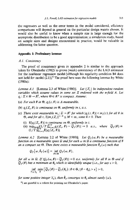
Appendix 1: Preliminary lemmas

A.1. Consistency

The proof of consistency given in appendix 2 is similar to the approach taken by Obenhofer (1982) to prove (weak) consistency of the LAD estimator for the nonlinear regression model [although his regularity condition B4 does not hold for model (2.1)].8 The proof here uses the following lemmas by White (1980a):

Lemma A.1 [Lemma 2.3 of White (1980)]. Let {Z,} be independent random variables which assume values in some set Z endowed with the a-jield A. Let

41 . - * = x 0 -+ R’, where 0 E Rr is compact. Assume:

(4

(b)

(4

For each 6 in 0, q,(z, 6) is A-measurable.

qt(Z,, t3) is continuous on 0, uniform& in t, a.s.

There exist measurable m,: E --, R’ for which [q,(.z, @)I < ml(z) for all 9 in 0, and for all t, E]m,(Z,)] ‘+’ I M < cc, some 6 > 0. Then

(9 Wq,(Z,, @>I IS continuous on 0, uniformly in t. (ii) supe,o](l/T)c~=,q,(Z,, @) - e,(S)] + 0 a.s., where QT(e) =

(l/T)C:&q,(Z,, Ql-

Lemma A.2 [Lemma 2.2 of White (1980)]. Let Qr(o, 8) be a measurable function on a measurable space 52 and for each w in J2 a continuous function of 0 on a compact set 0. Then there exists a measurable function e,(o) such that

for all w in 0. If lQr(o, 0) - Q,(S)1 + 0 a.e. uniformly for alI 8 in 0 and if Q&e) has a minimum at 8, which is identifiably unique (i.e., for any E > 0,

inf min{Q,(e)-Q,(e,):eEO,lle-eoll>E} >o, TrT, f3

for some positive integer T,), then 8, converges to t3, almost surety (w).

‘1 am grateful to a referee for pointing out Obenhofer’s paper.


A. 2. Asymptotic normality

The proof of asymptotic normality of & is based upon a simple extension of a theorem proved by Huber (1967) for maximum-likelihood-type estimation for i.i.d. samples. This theorem gives sufficient conditions under which a sequence of consistent estimators {Jr} which satisfy some ‘first-order condition’

is asymptotically normal, where the {Z,} are i.i.d. random variables taking values in some sample space z, and where J/ : Z x 0 --) RP is some given function, for 0 an open subset of Euclidean space R*.

For the estimator considered above, the corresponding random variables {Z,} are not identically distributed (although their mutual independence is assumed throughout), and in other applications the appropriate functions ( )C/((Zr, 8)} may vary systematically with the index t; nonetheless, Huber’s conditions can be easily modified to apply in such cases. Define

where the expectations here and throughout are taken with respect to the true distributions of the {Z,}, and let

The following conditions are imposed on lClr, A,, and pClr:

Assumption N.l. For each fixed B E 0 and each t, (p,(Z,, 0) is measurable, and $,( Z,, t9) is separable in the sense of Doob for all t: i.e., there is a countable subset 0’ C 0 such that for every open set U c 0 and every closed interval A, the sets {Z,: (I$I(Z,, @)(I E A, for all 0 c U} and {Z,: ll+,(Z,, f3)ll E A, for all B c Un 0’} differ at most by a set of (probability) measure zero.

Assumption N.Z. There is some 8, E 0 such that A,( aa) = 0 for T.

Assumption N.3. There are (strictly positive) numbers a, b, c, d,, and TO such that, for all t,

(0 ilW)il 2 a. 118 - 44 for ~~e-e,~~~d,, n To,

00 E[p,(Z,,6’,4Isb.d for 118 - solI + d I d,, d 2 0,

(iii) E[pI(Z,, 8, d)12 I c-d for ~l~--~,,ll+d~d,, dko.

J.L.. Powell, LAD estimation for regression models 317

Assumption N.4. Ell+,(Z,, e,,)l(’ 2 K for all t and some K> 0.

With these conditions, a simple asymptotic expression for A,(&) can be obtained.

Lemma A.3. Assume that Assumptions N.1 to N.4 hold and that

o/J?;)~~,(z,>~,)= o,(l) for 8,4,(z,,...,z,).

If 8, is consistent for 8, (i.e., Pr{ 118, - 8,l( > n} = o(1) for any TJ > 0), then

Proof. The method of proof is identical to that in Section 4 of Huber (1967). In each step of the proof of his Lemma 3, terms of the form

T.X(8), T-Ep(Z,B,d), etc.,

can be replaced by their ‘averaged’ counterparts

T.A,(@), C%(Z,, 8, d), etc.,

without affecting the validity of the argument if T is sufficiently large.

Appendix 2: Proofs of theorems in text

Proof of Theorem 1. Let

ur =yr- max{O, ,+,},

and define

h, = max(0, x:/3} - max{O, xX$,} = h,(P, Pa),

where

S=P-P,,

(A al)

(A.2)

(A-3)

here and throughout. Now minimization of S,(p) is equivalent to minimization of

eAs)=%t~)-S,t&), (A.4)

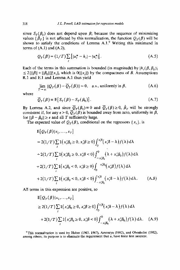
318 J. L. Powell, LAD esiimation for regression models

since S,(&) does not depend upon j3; because the sequence of minimizing values { &.} is not affected by this normalization, the function Q,(p) will be shown to satisfy the conditions of Lemma A.1.9 Writing this minimand in terms of (A.l) and (A.2),

Q&3)= (l/T)C[lu: - Wlu:k (A.5)

Each of the terms in this summation is bounded (in magnitude) by Ih,( j3, &,)I I 2[IIpII + II&ll]llx,II, which is O(llx,lj) by the compactness of B. Assumptions R.l and E-1 and Lemma A.1 thus yield

hm ~~Qr(~)-&(/3)~~=0, a.s.,uniformlyinP, (A.61 T-W

where

or(~) E E[%(P) - ~~Utdl. (A-7) By Lemma A.2, and since CT(&) = 0 and Q,(p) 2 0, p, will be strongly consistent if, for any E > 0, Q,(~) is bounded away from zero, uniformly in /3, for II/3 - &II 2 E and all T sufficiently large.

The expected value of Qr( /I), conditional on the regressors {x, >, is

E[Q~(P)I+.., xTI

=2(1/T)~l(n;/3,,~O,x;j3~0)/61:p(x;6-X)f(X)dh 1

+2(l/T)~l(x:P,~O,r:B<O)J_O~,~~(h+x:Po)/(X)dh I ,

+2(1/T)Cl(x;P,<O,~:P~O)So-~‘~‘(~~~)f(h)dh f

+2(1/T)Cl(x;P,<0,n;B<O)~~~~o(x;6-X)f(~)dX. (A.81 t :

All terms in this expression are positive, so

E[Q,(P)lxI~.4+1

2 2(1/T) x1( 44, 10, ~$3 r O)r( x;S - h)f( X) dX t

+2(1/T)C1(x:8,~0,~:8<O)J_~~~~(A+x~~~)~(A)dh. (A-9) t :

‘This normalization is used by Huber (1963, 1967), Amemiya (1982), and Obenhofer (1982), among others; its purpose is to eliminate the requirement that U, have finite first moment.

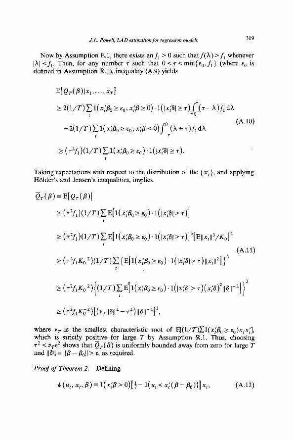
J.L. Powell, LAD estimation for regression models 319

Now by Assumption E.l, there exists an fi > 0 such that f( h) > fi whenever ]A 1 -c fi. Then, for any number 7 such that 0 < 7 < min{ .Q, fi } (where &cl is defined in Assumption R.l), inequality (A.9) yields

2 w7-)Cl(x:Po - >~~,x;PkO).l(Jx;Glt7)/‘(7--)fidh t 0

+2(l/WWx:P,~%, ~;fi<O)/~(A+T)f,dh (A.lO)

t -7

Taking expectations with respect to the distribution of the {xl}, and applying Holder’s and Jensen’s inequalities, implies

2 b2fiKT2)[(W12 - 72)llsll-2]3,

where vr. is the smallest characteristic root of E[(l/T)Cl(x;& 2 E,,)x~x$ which is strictly positive for large T by Assumption R.l. Thus, choosing 72 -C vr~~ shows that j&.(/3) is uniformly bounded away from zero for large T and (]6(] = ]]/I - &]] > E, as required.

Proof of Theorem 2. Defining

~(~,,xt,P)~l(X:B~O)[f-l(~t~X:(P-Po))lXt~ (A.12)

320 J.L. Powell, LAD estimation for regression models

the condition

must be established. Noting that the function # can be written as

(A.14)

it is easily verified that - 2T- f ‘kT( /I) is the vector of left partial derivatives of the objective function S&3) defined in (2.2) above. Because & minimizes S,(B), it is straightforward to show that ‘P,(&) satisfies

(A.15)

x ~[1(0<y,=x$r)+~~1(x;&=0)],

where the subscript j denotes the jth component of the corresponding vector [see Ruppert and Carroll (1980), proof of Lemma A.2, for demonstration of a similar result]. But max{ ]]x,]]: t I T} = o(n) almost surely by Assumption R.l, and the sum on the right-hand side of (A.15) is finite with probability one for all T suitably large by Assumptions E.l, R.2, and the strong consistency of a,. Thus condition (A.13) holds.

Next, conditions N.l though N.4 of Lemma A.3 must be established; only condition N.3 will be verified here, since the remaining conditions are easily checked. To show N.3(i) holds, it is convenient to write

tl/T)C-l(x:P>O).f(X~)x,x: (P-P,,), (A.16) I 1

where ‘E,’ denotes the expectation operator for the marginal distribution of x, and the {XT } are mean-value coefficients lying between zero and x:( p - &).


The second equality of (A.16) can be used to show

A,(D) -f(O)+&= OW - Poll), (A.17)

uniformly in T for /3 near /I,,, where M, is the matrix given in the statement of the theorem. This holds because each element of the difference satisfies

= (l/T)~E,[l(x:~‘O)[f(~~)-f(O)lx,,x~~ I

+[f(o)l(l/T)CE,[{l(x;~‘o)-l(x:P,’O)}x,,x,, I

2 wmEx[l(4P ’ O)lf( Y) -f(0)Illx,l?] (~4.18)

+ [f(o)l(l/T)CE,[l(lx:Pol~ llxrll IIP- Pclll)llxtl121 t

for II@ - &,I[ < So by Assumptions R.2 and E.2. Thus

MP) =f(O) %(P - PO) + NIP - POl12)~ (A.19)

and since the minimum characteristic root of Mr. is bounded above zero for all T sufficiently large (by Assumption R.l), inequality N.3(i) will be satisfied for all p in a sufficiently small neighborhood of &

To verify N.3@) and (iii), define

(A.20)

Then the definition of $ and some manipulation yields

P,(A 4 2 sup tllXtll* 1( l4Pl 2 IdP - Y > I) IIY-Bll<d

+ sup ll~,ll~~(l~,-~:PI~I~:~P-Y~l) lb-Bll<d

(A.21)

5 Ilx,ll[+ * 1( IxlPl 5 Iklld) + 1( 1% - x:PllI Ilx,lld)] ,


so

E[/-dP, d)] 5 [:K, +fo(f$)2’3] -d,

when IIP - &ll I &,, by Assumptions R.2 and E.1. Similarly,

(A.22)

E[dP, d)]* 5 [K, + V&,1 .d>

when II/3 - &II I lo, since pLt < 211x111 by (A.21).

Hence N.3 and the other conditions of Lemma A.3 hold, so

(A.23)

Conditions (A.19), (A.24), and the consistency of &- imply

@(8,-PII)= [f(o)~,1-‘(1/\lT)Cl(x:Po>o)

x [ $ - l( U, > o)] x, + o,(l). (A.29

The asymptotic normality of 8, then follows from the application of Liapunov’s central limit theorem to (A.25).

Proof of Theorem 3. Only the weak consistency of &-(0) will be demonstrated here; the convergence of M, to Ma can be proved in a similar fashion. First, the denominator of &.(O), when multiplied by l/T, can be replaced by (l/T)C Pr{ x$, > 0}, since

I(~/T)C[~(X:B,>O)-P~{~;B,>~}~( t

2 (l/T) x1( Ix:Pol 5 llxtll . II& - Poll)

+l(l/T)C[l(x;P,>O)-Pr{x;P,,>O}]/. t

(~.26)

The second term on the right-hand side is clearly o,(l); to show the first term

J. L. Powell, LAD estimqtion for regression models 323

also converges to zero in probability, note that, for any q> 0,

~~(~~/~~C~(l~~P,I~ll~rll~ll~r-Poll~~~}

~n((~/~~~~(l~~~~l~l~~tl~r),nj+~~~~l8~-ii,,~~ t

2 I-‘(l/T)C Pr{ I4Pd 2 IIxtllz} + Pr{ Ilk &II > 4 (A.27)

when z < &, which follows from Markov’s inequality and Assumption R.2(i). Thus, by choosing z sufficiently small, the right-hand side of (A.27) can be made arbitrarily small for large T by the consistency of 8,.

Similarly, the numerator, normalized by l/T, can be replaced by (c,T)- ‘cl< xi&, > 0). l(0 I U, I cr.), because plim &./c, = 1 and

These terms can each be shown to converge to zero in probability in the same fashion as in (A.27), using Assumptions R.2’ and E.2 and the facts that . c;‘ll&- &II = o,(l) and that c~‘li+-- cTI = o,(l). Now

E (c,T)-‘~l(x:Bo>0).1(O~u,I~,) [ t 1 = (l/T)x Pr{x$e> 0} l?c,‘f(h)dX

[ t 1 (l/T)C pr{x$0>0} /df(+h)dX

t 1 (A.29)

= (l/T)C Pr{ -Go > O} f(O) + o(l), t 1

324 J.L.. Powell, LAD estimation for regression models

by the dominated convergence theorem, and

= (f+T)-‘C var[l( ix& > 0). l(0 2 u, 2 Q.)]

~(c,T)~lc~‘Pr{O~u,~c,}=o(l/JT).

Hence

&(O)= (l/T)C Pr{xj&>O} +0,(l) -’ [ I 1

x f(O>(l/T)C Pr{ x2%> O} +-o,(l) [ ! 1

(A.30)

(A-31)

as asserted.

References

Amemiya, T., 1973, Regression analysis when the dependent variable is truncated normal, Econometrica 41, 997-1016.

Amemiya, T., 1982, Two stage least absolute deviations estimators, Econometrica 50, 689-711. Arabmazar, A. and P. Schmidt, 1981, Further evidence on the robustness of the Tobit estimator to

heteroskedasticity, Journal of Econometrics 17, 253-258. Arabmazar, A. and P. Schmidt, 1982, An investigation of the robustness of the Tobit estimator to

non-normality, Econometrica 50, 1055-1063. Bassett, G. and R. Koenker, 1978, Asymptotic theory of least absolute error regression, Journal of

the American Statistical Association 73, 667-677. Bickel, P.J., 1975, One-step Huber estimation in the linear model, Journal of the American

Statistical Association 70, 428-433. Buckley, J. and I. James, 1979, Linear regression with censored data, Biometrika 66, 429-436. Dempster, A.P., N.M. Laird and D.B. Rubin, 1977, Maximum likelihood from incomplete data via

the EM algorithm, Journal of the Royal Statistical Society B 39, l-22. Goldberger, A.S., 1980, Abnormal selection bias, Workshop paper no. 8006 (Social Systems

Research Institute, University of Wisconsin, Madison, WI). Hausman, J.A., 1978, Specification tests in econometrics, Econometrica 46, 1251-1271. Heckman, J., 1976, The common structure of statistical models of truncation, sample selection,

and limited dependent variables and a simple estimator for such models, Annals of Economic and Social Measurement 5, 475-492.

Heckman, J., 1979, Sample bias as a specification error, Econometrica 47, 153-162. Himmelblau, D.M., 1972, Applied nonlinear programming (McGraw-Hill, New York). Huber, P.J., 1964, Robust estimation of a location narameter. Annals of Mathematical Statistics

35, 73-101. Huber, P.J., 1965, The behavior of maximum likelihood estimates under nonstandard conditions,

Proceedings of the Fifth Berkeley Symposium 1, 221-233.


Jureckova, J., 1977, Asymptotic relations of M-estimates and R-estimates in the linear model, Annals of Statistics 5, 464-472.

Kalbfleisch, J.O. and R.L. Prentice, 1980, The statistical analysis of failure time data (Wiley, New York).

Kaplan, E.L. and P. Meier, 1958, Nonparametric estimation from incomplete observations, Journal of the American Statistical Association 53, 457-481.

Koenker, R. and G. Bassett, 1982a, Robust tests for heteroscedasticity based on regression quantiles, Econometrica 50, 43-61.

Koenker, R. and G. Bassett, 1982b, Tests of linear hypotheses and L1 estimation, Econometrica 50, 1577-1583.

Maddala, G.S. and F.D. Nelson, 1975, Specification errors in limited dependent variable models, National Bureau for Economic Research working paper no. 96.

Nelder, J.A. and R. Mead, 1965, A simplex method for function minimization, The Computer Journal 7, 308-313.

Obenhofer, W., 1982, The consistency of nonlinear regression minimizing the L1 norm, Annals of Statistics 10, 316-319.

Parzen, E., 1962, On estimation of a probability density function and its mode, Annals of Mathematical Statistics 33,1065-1076.

Powell, J.L., 1983, The asymptotic normality of two-stage least absolute deviations estimators, Econometrica 51,1569-1575.

Powell, M.J.D., 1964, An efficient method for finding the minimum of a function of several variables without calculating derivatives, The Computer Journal 7, 155-162.

Robinson, P.M., 1982, On the asymptotic properties of estimators of,models containing limited dependent variables, Econometrica 50,27-41.

Ruppert, D. and R.J. Carroll, 1980, Trimmed least squares estimation in the linear model, Journal of the American Statistical Association 75, 828-838.

Taylor, L.D., 1974, Estimation by minimizing the sum of absolute errors, in: P. Zarembka, ed., Frontiers in econometrics (Academic Press, New York).

Tobin, J., 1958, Estimation of relationships for limited dependent variables, Econometrica 26, 24-36.

White, H., 1980a, Nonlinear regression on cross-section data, Econometrica 48, 721-746. White, H., 1980b, A heteroskedasticity-consistent covariance matrix estimator and a direct test for

heteroskedasticity, Econometrica 48, 817-838.

least absolute deviations estimation for the censored

Documents