least constraining time-slot allocation in gmpls …bochmann/curriculum/pub/theses/phd-theses... ·...
TRANSCRIPT

Least Constraining Time-Slot Allocation in
GMPLS Optical TDM Networks
and
Optimization of Optical Buffering
Hassan Zeineddine
Thesis submitted to the Faculty of Graduate and Postdoctoral Studies
in partial fulfillment of the requirements for the PhD degree in
Computer Science
Ottawa-Carleton Institute for Computer Science
School of Information Technology and Engineering Faculty of Engineering University of Ottawa
© Hassan Zeineddine, Ottawa, Canada, 2009

ii
Abstract
Optical Time Division Multiplexing (OTDM) in optical networks is a bandwidth sharing
technique that organizes access to a shared wavelength in equal time-slots organized in
repeated frames. In this case, a transmission channel can be established at the time-slot
level instead of using the full wavelength. The main advantage of this technique is to allow
several low speed communication channels to coexist on the same high speed optical
wavelength, and hence to make effective use of the enormous bandwidth available on a
single wavelength. On the other hand, the major problem with OTDM is the time slot
continuity constraint in an OTDM channel, which is similar to the wavelength continuity in
a WDM channel. Due to this constraint, time slot contentions can exist in the network if
proper scheduling and slot reservation techniques are not employed. Basically, the adopted
time slots must be free on all links throughout the communication route in order to
successfully reserve a communication channel. In addition, to mitigate the effect of slot
continuity constraint on bandwidth utilization, appropriate time slot buffering (or
interchanging) is often employed. Previous work assumed the deployment of Optical
Time-Slot Interchangers (OTSI) to solve the contention problems regardless of their
industrial feasibility. In addition, other work considered very basic reservation schemes to
achieve proper scheduling, such as the First Fit (FF), Random Fit (RF), and Least Loaded
(LL) schemes. In this thesis, we propose a new time-slot reservation scheme for OTDM
networks without buffering to significantly improve the performance and eliminate the
buffering overhead. It is the Least Constraining (LC) slot reservation scheme which
allocates resources having the lowest possible constraints on other resources in the
network. In addition, we define a distributed scheme to deploy the LC approach in GMPLS
networks, and prove that the same performance level can be maintained by a distributed
signaling protocol. Finally, we propose an optimized optical buffering technique to achieve
close to optimum performance when the LC reservation approach is not used. It helps in
building effective time slot synchronization devices used between adjacent node pairs.

iii
Table of Contents
1. INTRODUCTION ................................................................................................................................... - 1 -
1.1. PROBLEM STATEMENT ........................................................................................................................ - 2 - 1.2. MOTIVATION AND OBJECTIVES ........................................................................................................... - 3 - 1.3. LIST OF CONTRIBUTIONS .................................................................................................................... - 3 - 1.4. OUTLINE ............................................................................................................................................. - 4 -
2. BACKGROUND ...................................................................................................................................... - 6 -
2.1. OTDM NETWORK ARCHITECTURE ..................................................................................................... - 6 - 2.2. OTDM NODE ARCHITECTURE .......................................................................................................... - 11 - 2.3. ARCHITECTURE OF OPTICAL TIME SLOT INTERCHANGERS ............................................................... - 13 - 2.4 OPTICAL TIME SLOT RESERVATION SCHEMES ................................................................................... - 17 -
2.4.1. Optical Time Slot Reservation Based on Frame Boundary Synchronization ........................... - 17 - 2.4.2. Optical Time Slot Reservation Based on Slot Boundary Synchronization ............................... - 21 - 2.4.3. Optical Time Slot Reservation with QoS consideration ........................................................... - 23 - 2.4.4. Distributed Optical Time Slot Reservation .............................................................................. - 24 -
2.5. MULTI-PROTOCOL LABEL SWITCHING ............................................................................................. - 33 - 2.5.1. MPLS Header .......................................................................................................................... - 34 - 2.5.2. Resource Allocation in MPLS .................................................................................................. - 34 - 2.5.3. Resource Update in MPLS ....................................................................................................... - 35 - 2.5.4. Generalized MPLS ................................................................................................................... - 36 -
3. LEAST CONSTRAINING SLOT ALLOCATION ............................................................................ - 37 -
3.1. PROBLEM DEFINITION ...................................................................................................................... - 37 - 3.2.1. Basic Concepts ......................................................................................................................... - 38 - 3.2.2. Basic Definitions .................................................................................................................... - 39 - 3.2.2.1. Resource Availabilities ......................................................................................................... - 39 - 3.2.2.2. Intersecting Route-Slot Sets .................................................................................................. - 40 - 3.2.2.3. Resource Constraint.............................................................................................................. - 41 - 3.2.3. Allocation Principle ............................................................................................................... - 42 - 3.2.4. Constraint Update .................................................................................................................. - 42 - 3.2.5. Illustrative Example ................................................................................................................. - 44 -
3.3. SIMULATION RESULTS ...................................................................................................................... - 46 - 3.3.1. Simulation ................................................................................................................................ - 46 - 3.3.2. Observations ............................................................................................................................ - 49 -
3.4. ANALYTICAL DISCUSSION ................................................................................................................ - 56 - 3.5. CONCLUSION .................................................................................................................................... - 66 -
4. DISTRIBUTED ALGORITHM FOR THE LEAST CONSTRAINING SLOT ALLOCATION SCHEME IN A GMPLS CONTEXT ...................................................................................................... - 68 -
4.1. INTRODUCTION ................................................................................................................................. - 68 - 4.2. DISTRIBUTED APPROACH ................................................................................................................. - 69 -
4.2.1. Node Database ......................................................................................................................... - 69 - 4.2.2. Reservation process ................................................................................................................. - 71 - 4.2.3. Resource Status Update ........................................................................................................... - 74 - 4.2.3.1. Immediate Resource Status Update ...................................................................................... - 74 - 4.2.3.2. Periodic Resource Status Update ......................................................................................... - 75 - 4.2.4. Backward vs. Forward Reservation ......................................................................................... - 76 -
4.3. SIMULATION RESULTS ...................................................................................................................... - 76 - 4.4. ANALYTICAL DISCUSSION............................................................................................................... - 85 - 4.5. CONCLUSION ................................................................................................................................... - 90 -

iv
5. VARIATIONS OF THE LEAST CONSTRAINING SLOT ALLOCATION SCHEME ............... - 91 -
5.1. PROBLEM DEFINITION ...................................................................................................................... - 91 - 5.2. RESOURCE CONSTRAINT DEFINITION VARIATIONS ......................................................................... - 93 -
5.2.1. Constraint Definition for LC Based on Route-Slot Count (LCv1) ......................................... - 93 - 5.2.2. Constraint Definition for LC Based on Availability Ratio (LCv2) ......................................... - 94 - 5.2.3. Illustrative Example ................................................................................................................. - 95 -
5.2. ESSENTIAL CHANGES TO THE RESOURCE CONSTRAINT UPDATE MODULE ...................................... - 96 - 5.2.1. Constraint Update Change for LCv1 ..................................................................................... - 97 - 5.2.1.2. Distributed Approach ............................................................................................................ - 98 - Immediate Resource Status Update ................................................................................................... - 98 - Periodic Resource Status Update ...................................................................................................... - 99 - 5.2.2. LCv2 Update Module change .............................................................................................. - 100 - 5.2.2.2. Distributed Approach .......................................................................................................... - 101 -
5.3. SIMULATION RESULTS .................................................................................................................... - 101 - 5.4. CONCLUSION .................................................................................................................................. - 106 -
6. OPTIMIZED PASSIVE OPTICAL TIME-SLOT INTERCHANGER ......................................... - 108 -
6.1. INTRODUCTION ............................................................................................................................... - 108 - 6.2. LIMITED-RANGE POTSI (POTSI-LR) ............................................................................................ - 109 - 6.3. SHARED SWITCH ARCHITECTURE ................................................................................................... - 110 - 6.4. OTSI VS WAVELENGTH CONVERTER ............................................................................................. - 112 - 6.5. POTSI BASED SYNCHRONIZERS ..................................................................................................... - 113 - 6.6. BANDWIDTH ALLOCATION WITH SHARED LIMITED-RANGE POTSIS ................................................ - 114 - 6.7. CONCLUSION .................................................................................................................................. - 119 -
7. CONCLUSIONS .................................................................................................................................. - 121 -
7.1. SUMMARY ...................................................................................................................................... - 121 - 7.2. OVERVIEW OF CONTRIBUTIONS ...................................................................................................... - 124 - 7.3. FUTURE WORK ............................................................................................................................... - 126 -
REFERENCES ........................................................................................................................................ - 128 -

v
LIST OF FIGURES
FIGURE 2.1: EXAMPLE OF AN OTDM MESH NETWORK ................................................................................... - 7 - FIGURE 2.2: TIME SLOT’S GRAPHICAL DESCRIPTION ....................................................................................... - 8 - FIGURE 2.3: AN OPTICAL NETWORK BASED ON THE TWIN ARCHITECTURE ................................................. - 10 - FIGURE 2.4: ALL-OPTICAL STAR NETWORK ARCHITECTURE ......................................................................... - 11 - FIGURE 2.5: AN OTDM SWITCH ARCHITECTURE .......................................................................................... - 13 - FIGURE 2.6: INTERNAL ARCHITECTURE OF A 1,2, …, N-1 OTSI ................................................................... - 15 - FIGURE 2.7: INTERNAL ARCHITECTURE OF A PASSIVE OTSI ........................................................................ - 16 - FIGURE 2.8: FORWARD RESERVATION USE CASES......................................................................................... - 26 - FIGURE 2.9: BACKWARD RESERVATION USE CASE ........................................................................................ - 29 - FIGURE 2.10: ARM COMMUNICATION USE CASES ........................................................................................ - 32 - FIGURE 2.11: MPLS HEADER....................................................................................................................... - 34 - FIGURE 2.12: MPLS RESERVATION PROCESS ............................................................................................... - 35 - FIGURE 2.13: HIERARCHICAL LSPS IN GMPLS ........................................................................................... - 36 - FIGURE 3.1: CONSTRAINT UPDATE ALGORITHM ........................................................................................... - 43 - FIGURE 3.2: CONSTRAINT UPDATE ALGORITHM ........................................................................................... - 44 - FIGURE 3.3: A ROUTE-SLOT (
10EF ) AND ITS RELATED LINK-SLOTS .............................................................. - 45 - FIGURE 3.4: NSFNET TOPOLOGY ................................................................................................................ - 47 - FIGURE 3.5: A 14-NODE RING TOPOLOGY ..................................................................................................... - 47 - FIGURE 3.6: A 14-NODE STAR TOPOLOGY ..................................................................................................... - 48 - FIGURE 3.7: LC VS. FF WITH UNIFORM TRAFFIC ........................................................................................... - 50 - FIGURE 3.8: LC VS FF WITH NON-UNIFORM TRAFFIC ................................................................................... - 51 - FIGURE 3.9: COMPARING LC TO LL IN MULTI-FIBER NETWORKS (3 FIBERS PER LINK) ................................. - 52 - FIGURE 3.10: LC VS FF WITH 2 ALTERNATIVE-PATHS ROUTING ................................................................... - 53 - FIGURE 3.11: LC PERFORMANCE IN 14-NODE RING NETWORK ...................................................................... - 54 - FIGURE 3.12: MEASURING LC IN A STAR NETWORK ..................................................................................... - 55 - FIGURE 3.13: LC PERFORMANCE AFTER FACTORING THE LOAD IN THE RESOURCE CONSTRAINTS ................ - 56 - FIGURE 3.14: PERCENTAGE OF LINK-SLOTS HAVING LOW, AVERAGE, AND HIGH CONSTRAINTS ................... - 61 - FIGURE 3.15: ANALYTICAL RESULTS OF THE LC APPROACH IN A MULTI-FIBER NETWORK ........................... - 65 - FIGURE 3.16: ANALYTICAL RESULTS OF THE LC APPROACH IN A SINGLE-FIBER NETWORK .......................... - 66 - FIGURE 4.1: NODAL DATABASE HIERARCHY ................................................................................................ - 70 - FIGURE 4.2: RESERVATION USE CASE ........................................................................................................... - 73 - FIGURE 4.3: LC PERFORMANCE FOR DIFFERENT UPDATE RATES (ONCE PER 1E+X CALLS) – WITH UNIFORM
TRAFFIC .............................................................................................................................................. - 77 - FIGURE 4.4: LC PERFORMANCE FOR DIFFERENT UPDATE RATES (ONCE PER 1E+X CALLS) – WITH NON-UNIFORM
TRAFFIC .............................................................................................................................................. - 78 - FIGURE 4.5: LC PERFORMANCE MEASURED EVERY 10 CALLS – LOAD IS 120 ERLANG – (UPDATE RATE IS ONCE
EVERY 500 CALLS) .............................................................................................................................. - 79 - FIGURE 4.6: LC PERFORMANCE MEASURED EVERY 10 CALLS – LOAD IS 120 ERLANG –(UPDATE RATE IS NONE
FOR THE FIRST AND LAST 500 CALLS, AND IMMEDIATE UPDATES FOR THE MIDDLE 500 CALLS) .......... - 81 - FIGURE 4.7: LC PERFORMANCE MEASURED EVERY 10 CALLS – LOAD IS 120 ERLANG –(WITH TWO DIFFERENT
TRAFFIC PATTERNS) ............................................................................................................................ - 83 - FIGURE 4.8: LC PERFORMANCE FOR DIFFERENT UPDATE RATES (ONCE PER 1E+X CALLS) IN A 3-FIBERS
NETWORK ........................................................................................................................................... - 84 - FIGURE 5.1: EXAMPLE OF THE CONSTRAINT CALCULATION FOR LCV1 AND LCV2 ....................................... - 96 - FIGURE 5.2: CONSTRAINT UPDATE ALGORITHM AFTER RESERVATION OF A CALL ......................................... - 97 - FIGURE 5.3: CONSTRAINT UPDATE ALGORITHM AFTER RELEASE OF A CALL ................................................. - 98 - FIGURE 5.4: CONSTRAINT UPDATE ALGORITHM AFTER RESERVATION OF A CALL ....................................... - 100 - FIGURE 5.5: CONSTRAINT UPDATE ALGORITHM ......................................................................................... - 101 - FIGURE 5.6: PERFORMANCE OF ALL LC APPROACH VARIATIONS IN A SINGLE-FIBRE ENVIRONMENT ......... - 102 - FIGURE 5.7: PERFORMANCE OF THE LC APPROACH VARIATIONS IN A MULTI-FIBER NETWORK ................... - 103 - FIGURE 5.8: PERFORMANCE OF THE DISTRIBUTED LC APPROACH WITH DIFFERENT VARIATIONS IN A MULTI-
FIBER NETWORK (WITH NO UPDATES) ............................................................................................... - 105 -

vi
FIGURE 5.9: PERFORMANCE OF THE DISTRIBUTED LC APPROACH WITH DIFFERENT VARIATIONS IN A MULTI-FIBER NETWORK (WITH UPDATE RATE OF 1 PER 103
CALLS) .............................................................. - 106 - FIGURE 6.1: A LIMITED RANGE POTSI WITH 3 FDLS INSTEAD OF N-1 ...................................................... - 110 - FIGURE 6.2: DEDICATED POTSI ARCHITECTURE OF A 4 X 4 SWITCH ......................................................... - 111 - FIGURE 6.3: SHARED OTSI ARCHITECTURE OF A 4 X 4 SWITCH HAVING 2 POTSIS ................................... - 111 - FIGURE 6.4: SCHEMATIC REPRESENTATION OF A POTSI-BASED SYNCHRONIZER ....................................... - 114 - FIGURE 6.5: THE EFFECTS OF VARYING THE POTSI’S SHARING-PERCENTAGES (S%) AND INTERCHANGING
RANGES (R%) IN NSF NETWORK ...................................................................................................... - 115 - FIGURE 6.6: THE EFFECTS OF VARYING POTSI’S SHARING-PERCENTAGE (S%) AND INTERCHANGING RANGE IN
A STAR NETWORK OF 20 EDGE NODES, WITH LOAD 60 ERLANG ........................................................ - 116 - FIGURE 6. 7: BLOCKING PROBABILITY IN A 14-NODES RING TOPOLOGY, WHEN INTERLEAVING POTSIS
AMONGST NODES AT DIFFERENT RATE (I) ......................................................................................... - 117 - FIGURE 6.8: BLOCKING PROBABILITY IN A 14-NODES RING TOPOLOGY, WHEN VARYING THE POTSIS
INTERLEAVING RATE BETWEEN 0 AND 1, AT A FIXED LOAD OF 35 ERLANG ...................................... - 118 - FIGURE 6.9: BLOCKING PROBABILITY IN A 14-NODE RING TOPOLOGY, WITH POTSI’S INTERLEAVING RATE (I)
0.5, AND VARIOUS PERCENTAGES OF INTERCHANGING RANGES (R%) ............................................... - 119 -

vii
LIST OF TABLES
TABLE 2.1: CHARACTERISTICS OF VARIOUS OTSI ARCHITECTURES ............................................................. - 17 - TABLE 4.1: PROBABILITY SYMBOLS ............................................................................................................. - 85 - TABLE 4.2: ANALYTICAL RESULTS ............................................................................................................... - 89 - TABLE 5.1: RESULTS FROM FIGURE 5.1 ........................................................................................................ - 95 - TABLE 6.1: OTSI ARCHITECTURE COMPARISON ........................................................................................ - 109 -

viii
ACRONYM
CRA Conflict Resolution Algorithm CR-DP Constraint-Based Routing LDP CRSL Common Route-Slots List
ESP Expanded Shortest-Path FDL Fiber Delay Line
FF First Fit GMPLS Generalized Multi-Protocol Label Switching
IS-IS Intermediate System to Intermediate System LAN Local Area Network
LC Least Constraint LDP Label Distribution Protocol LER Labeled Edge Router LIL Links Info List LL Least Loaded
LSAL Link-Slot Availability List LSIL Link-Slots Info List LSP Label Switched Path LSR Label Switched Router
MAN Metropolitan Area Network MCS Minimum-Cost Search
MPLS Multi-Protocol Label Switching OBS Optical Burst Switching OPS Optical Packet Switching
OSPF Open Shortest Path First OTSI Optical Time-Slot Interchanger PIM Parallel Iterative Matching
POTSI Passive Optical-Time Slot Interchanger POTSI-LR Limited Range Optical-Time Slot Interchanger
QBvN Quick Birkhoff-von Neumann RF Random Fit
RSCL Route-Slot Constraint List RSVP Resource Reservation Protocol
RSVP-TE RSVP with Traffic Engineering RWTA Routing, Wavelength and Time-slot Assignment
SABCA Slot Assignment Based on Capacity Allocation SABPA Slot Assignment Based on Packet Arrival
TDM Time Division Mutliplexing TWIN Time-domain Wavelength Interleaved Networking
TWIN-WR TWIN with Wavelength Reuse WAN Wide Area Network WDM Wavelength Division Multiplexing

ix
ACKNOWLEDGMENTS
“And We have enjoined upon man concerning his parents - His mother beareth him in weakness upon weakness, and his weaning is in two years - Give thanks unto Me and unto
thy parents. Unto Me is the journeying.” (Quraan 31\14). الشكر لك يا رب This written thesis is the harvest of many years of research and investigations. I definitely would not be writing the acknowledgements paragraph without the support of my supervisor Dr. Gregor v. Bochmann. I am extremely blessed to work with such a shrewd thinker and critical observer who enriched this work with his valuable comments and guidance. I would also like to thank my thesis committee members for their time spent reading and discussing this work. My indescribable gratitude is to my Mom (hajja Mariam) and Dad (hajj Fadl) for seeding the stamina for knowledge in me. They are my reason for being and hence I owe them my accomplishments in life including this work. All thanks goes to my beloved wife Manal. Her patience and support throughout my years of study were priceless. No matter what I do in return would not equally reward her. I know that her understanding and help were unconditional; however, maybe if I do the dishes for a few days, I could settle the score!! I should not forget to thank my two little daughters Aya and Zeinab for being my joy and stress busters. I would also like to thank my parent in-laws for making life easier on me with their much appreciated help in various aspects of my day to day living. Finally, I express my gratitude to each and every member of my family and in-laws for their encouragements and faith in me. In addition, I shall thank all my friends for their support.

- 1 -
1. Introduction
With the massive deployment of Wavelength Division Multiplexing (WDM) systems
[Ramaswami2002], researchers have shown increased interests in studying the question of
wavelength sharing. As the transmission capacity over a single wavelength is in the order
of 10 Gigabits per second (Gbs), the resulting bandwidth has exceeded the aggregated
traffic load of many source nodes. Thus, dedicating one wavelength for a single end-to-end
connection with low load is like shipping a small envelop with an empty plane; that is.,
only a slim share of the bandwidth is being utilized while the rest remains untapped. To
maximize bandwidth utilization, researchers worked under three major research streams
focused on wavelength sharing: Optical Packet Switching (OPS), Optical Burst Switching
(OBS), and Optical Time Division Multiplexing (OTDM).
Optical packet switching is achieved in an optical network by switching optical traffic units
(packets) in the optical layer without opto-electronic conversion [Blumenthal1994,
Yao2000, Pattayina2000]. Each packet must carry its addressing information in a header.
Intermediate nodes are supposed to read the header, decide the next node in the
corresponding route, and configure its cross-connect switch accordingly in a relatively
short period of time. They should also be capable of storing contending packets in optical
buffers. In fact, the header processing speed and optical buffering are two major challenges
facing the realization of OPS. No matter how fast the header processing speed gets, it
remains bound to the electronic speed; and hence, it is way too slow compared to the
optical speed. In addition, optical buffering is still immature to handle randomized access.
It seems that the road is still long before reaching the OPS goal.
While waiting for a breakthrough in OPS, Optical Burst Switching [Turner1999,
Qiao1999, Vokkarane2003] seems to offer an interim solution. With OBS, a burst of traffic
containing several packets is aggregated electronically at the source node before being sent
optically in the network. It is an attempt to benefit from electronic buffering at the source
before sending traffic through the optical network. In addition, the packet header is

- 2 -
replaced with a control header that travels ahead of time on a separate control channel. The
control header is used to reserve resources on intermediate switches for a limited period,
enough to forward the corresponding traffic burst. If a network resource happens to be
busy or faulty, the burst is dropped. Clearly, a major disadvantage of OBS is the steep
increase in packet loss as the traffic load gets higher. Several enhancements were
introduced to reduce contention and improve loss ratio. Deflection routing, wavelength
conversion, and optical buffering are the main contention resolution techniques
[Maach2004].
Another candidate for filling the time gap between now and the emergence of OPS is
Optical Time Division Multiplexing (OTDM) [Liew2003]. It reduces the granularity of
traffic segments traveling in the network, maximizes bandwidth utilization, and reduces
contention by proper scheduling. OTDM allows several connections to coexist on the same
wavelength in a repeating frame of N time slots. Similar to the wavelength continuity
constraint in wavelength routed networks, time slot continuity is essential in OTDM
networks. To mitigate the effect of the slot continuity constraint on bandwidth utilization,
appropriate time slot buffering (or interchanging) is described in the literature.
1.1. Problem Statement Most of the optical time slot allocation schemes found in the literature are based on the
First Fit or Random Fit allocation schemes [Zang1999, Zang2000, Huang2000, Liew2003,
Maach2004, Yates2004, Wen2005, Yang2007a, Yang2007b]. Just one single work
[Wen2005] adopted the Least Loaded scheme. In this thesis, we propose a new bandwidth
allocation scheme to improve network performance in OTDM networks to a level close to
optimum. We also define a distributed scheme for practical deployment of the new solution
in a GMPLS network while maintaining the same improvement of performance. Although,
the proposed solution should eliminate the need for optical buffering as it yields close to
optimal performance, we also propose a new optimized optical buffering technique and
related switch architecture.

- 3 -
1.2. Motivation and objectives Motivated by the goal to find a slot allocation solution in OTDM networks that improves
performance to a level close to optimum, we designed a scheme that reserves bandwidth
resources having the least constraints on other dependent resources. It is what we call the
Least Constraining (LC) slot allocation technique, where the slot constraint is measured by
the number of available transmission channels on the fixed routes that can use this slot at a
given point in time. In addition, influenced by the GMPLS protocol for optical networks
[Colle2003, RFC3945], we define a distributed scheme to deploy the LC slot allocation
technique in GMPLS networks. We focus on the resource state update aspect of the
distributed scheme as it is a key factor for network scalability and compatibility with
GMPLS. Although, the LC allocation approach should eliminate the need for buffering as a
means to enhance performance, we propose an optimized buffering technique and
corresponding switch architecture in optical TDM networks. We also describe the possible
usage of the optimized buffering technique to synchronize transmission between two
adjacent nodes (connected by a direct link).
1.3. List of Contributions We identify the following items as the main contributions discussed in this thesis:
1. The Least Constraining Slot Allocation Scheme – which provides a performance
close to the optimal performance achieved with full buffering at each node – in
Chapter 3.
2. The Distributed Least Constraining Slot Allocation Scheme – an approach to
deploy the LC scheme in a GMPLS environment while maintaining close to
optimum performance – in Chapter 4.
3. Several variations of the LC scheme and their comparison – to identify the variant
that achieves the best performance – in Chapter 5.

- 4 -
4. Limited Range Passive Optical Time Slot Interchanger – a novel optimized optical
buffering technique which provides the same performance achieved with traditional
OTSI – in Chapter 6.
5. Shared Passive OTSI architecture – a novel OTDM switch architecture based on a
pool of shared OTSIs instead of a dedicated OTSI per input line as known in the
literature – described in Chapter 6.
6. Interleaved Passive OTSI in OTDM networks – a novel proposal to interleave
OTSIs among network nodes instead of deploying these buffering devices at each
node – in Chapter 6.
7. Effective slot synchronization technique based on the Passive OTSI architecture – a
new solution for the synchronization problem between two adjacent nodes in an
OTDM network – in Chapter 6.
1.4. Outline The thesis is made of 7 chapters and is structured as follows:
- Chapter 1 is the introduction.
- Chapter 2 provides a literature review of the technologies being investigated or adopted,
namely OTDM network components, time slot reservation schemes, and GMPLS.
- Chapter 3 introduces the novel Least Constraining Slot Allocation scheme, which
achieves a performance close to the optimal performance achieved with full buffering at
each node. Simulation results, backed by analytical discussion, are used to measure the
network performance under various topologies and different routing approaches.
- Chapter 4 discusses the deployment of the LC scheme in a GMPLS network. It
describes a distributed algorithm for resource reservation; however, the focus is on
minimizing the rate of status updates, which has a major impact on scalability and
compatibility with GMPLS.
- Chapter 5 lists and compares 3 different variations of the original LC approach. It
identifies the variation that achieves the best network performance.

- 5 -
- Chapter 6 proposes an optimized optical time slot interchanging technique based on the
Passive OTSI architecture described in a previous work [Maach2004]. It studies the
effect of reducing the range and number of OTSIs in the network in terms of
performance. In addition, it describes the effective usage of Passive OTSI as
synchronizing devices between two adjacent nodes in an OTDM network.
- Chapter 7 concludes the thesis by summarizing the characteristics and achieved results
of each contribution. It also discusses potential future extensions to investigate some
topics that are not covered in this work.

- 6 -
2. Background In this chapter, we review the major aspects of OTDM with special emphasis on slot
scheduling schemes. The content is organized in the following order: OTDM networks,
OTDM switch architectures, optical time slot interchangers, slot reservation schemes, and
a brief introduction to MPLS.
2.1. OTDM Network Architecture As we briefly described in the introduction, the OTDM technique multiplexes low rate
traffic streams in frames of N time slots over a high speed wavelength. I.e., up to N
different streams can be carried over a single wavelength. Each stream is assigned one time
slot in a frame over a given wavelength. Note that a connection can use multiple streams
[Liew2003]. The stream bandwidth in the network is N
1 of the wavelength bandwidth. For
example, if a frame is made of 1000 time slots and the wavelength speed is 10 Gbps, then
the stream bandwidth is 10 Mbps. Figure (2.1) is a graphical example of an optical TDM
network.

- 7 -
Figure 2.1: Example of an OTDM mesh network
OTDM networks fall under two major categories, mesh and star. In an OTDM mesh
network, every node is equipped with an optical cross-connect that maps inputs to outputs
according to a defined schedule. The schedule is updated according to the employed slot
reservation scheme. It reflects the switching pattern for a time slot period, when traffic
segments entering the switch are switched to the corresponding output. It is essential that
all traffic segments within a slot period reach the cross-connect right at the beginning of a
new time slot. In addition, the cross-connect must transition to the next state right before
the start of a new time slot.
To achieve synchronization between segments arrival and switch state during a time slot,
several solutions were introduced in the literature: 1- clock alignment plus precise fiber
cut, and 2- use of input synchronizers.
For the first approach, all nodal clocks are synchronized to advance simultaneously from
one slot to another. This can be achieved by broadcasting a clock signal from a central
station to all nodes so that they can adjust their clock accordingly. In addition, all fibers
λ1
λ2TDM Frame of N timeslots
Parallel frames on 2 different wavelengths
Traffic load in a timeslot
All-optical TDM node
Fiber link

- 8 -
between adjacent nodes must be carefully cut to round up the propagation delay to the
nearest integer in order to attain slot boundary alignment. In this case, a transmitted traffic
segment is always guaranteed to reach the next cross-connect on a route at the start of a
time slot. A slight slot misalignment might arise due to inaccurate fiber cutting, minor
clock difference, or changing propagation delays due to temperature changes. This
imperfection can be solved by defining an offset period as a guard time at each slot as
shown in Figure (2.2). In addition to slot misalignment, the guard time must account for
the cross-connect reconfiguration time when transitioning from one slot to another. The
remaining part of a time slot would be the effective bandwidth that carries the traffic
segments. For example, if the maximum tolerated error in fiber cutting is 10m and the
switch reconfiguration time is 0.05μs the guard time must be 10 ⁄ (2 × 10⁸)s + 0.05μs =
0.05μs + 0.05μs = 0.1μs, which is 1% of a 10μs time slot. To eliminate the configuration
time from the formula, a switch architecture with two parallel-planes is required. When one
switching plane is handling traffic, the other would be reconfiguring to be ready for traffic
at the next time slot, and vice versa. Note that the slot time must be larger or equal to the
reconfiguration time.
Figure 2.2: Time slot’s graphical description
Timeslot
Guard time
Reconfiguration time

- 9 -
As for the second synchronization approach, special all-optical devices known as
synchronizers are deployed at every switch’s input [Ramamirtham2003]. A synchronizer
delays incoming traffic by a pre-calculated period to offset the lag caused by clocks
difference and propagation delays. Details are described in Section 2.3.
A Photonic Slot Routing mesh network is one of the OTDM network architectures
described in the literature [Zang2000] and [Zang1999]. In this approach, packets going to
the same destination and traveling on different wavelengths during a common time slot are
treated as an integral unit at intermediate switches. In this case, there is no need to de-
multiplex and multiplex wavelengths at intermediate nodes along the route to its
destination. Multiplexing and de-multiplexing are only required when the packet is
submitted or received. In addition, intermediate nodes can transmit traffic to a given
destination node D on a free wavelength λ during a photonic slot t if the traffic unit in t is
headed to node D.
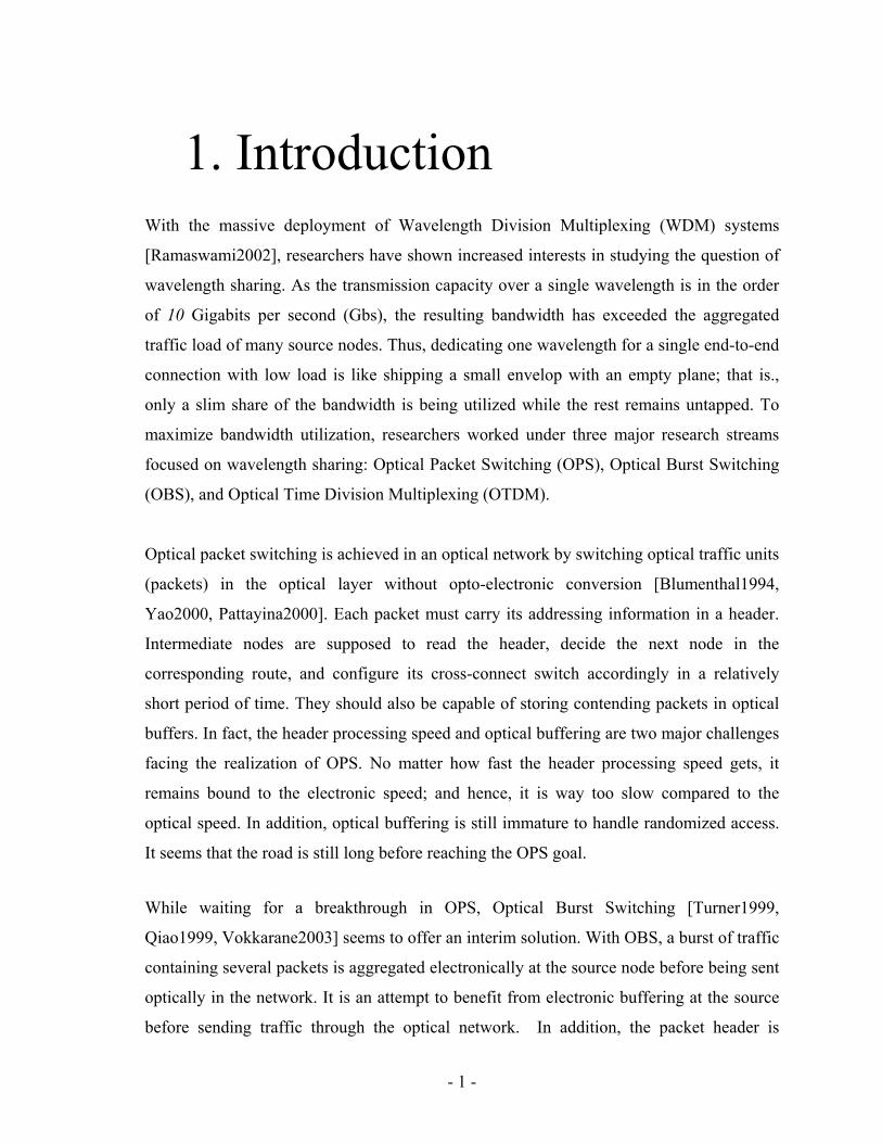
In [Widjaja2004], the Time-domain Wavelength Interleaved Networking (TWIN) was
introduced. The TWIN architecture provides time-shared connectivity using static switches
and dynamic tunable transmitters. Each node is assigned a unique wavelength on which it
would receive incoming traffic. In addition, all nodes are pre-configured to switch every
wavelength to its assigned node. See Figure (2.3) for details. In this case, if a node S has to
send traffic to node D, it tunes its transmitter to the wavelength assigned to D, and starts
transmitting at a given time slot. Dynamic signaling and fast switching are not required to
reconfigure intermediate nodes since all intermediate resources are statically allocated to
lead the traffic to node D. The major limitation with this architecture is scalability. A
network cannot include a number of nodes that exceeds the available number of supported
wavelengths. In addition, a wavelength bandwidth is not efficiently utilized especially
when a destination is not receiving traffic from any source.
- 10 -
Figure 2.3: An optical network based on the TWIN architecture
To support larger networks and make better use of the bandwidth, an enhanced version of
TWIN with wavelength reuse (TWIN-WR) was proposed in [Nuzman2006]. Basically,
TWIN-WR suggests re-using a wavelength in network areas where it is not utilized. The
authors described the basic TWIN connection between two nodes without wavelength
reuse as single hop although these nodes might be interconnected by several links. Their
concept of a hop is a direct line of light between two nodes without opto-electronic or
optical switching. On the other hand, they see a TWIN-WR connection as a sequence of
one or more basic TWIN connections between a source destination pair, i.e. a multi-hop
connection. Nuzman et al. assumed a form of traffic relay is in place at each node to
achieve bridging between hops. With this, they were able to support a network of N nodes
with roughly N wavelengths.
In [Bochmann2004], an OTDM star network was proposed. In this network, the core node
has an active all-optical cross-connect that is configured at each time slot based on a given
schedule. Edge nodes are connected to the core, and equipped with transceivers to send and
receive traffic segments through the core. A graphical example is shown is Figure (2.4). In
Tx Rx
Optical Switch
Bi-directional link
λ1
λ2

- 11 -
this network, accurate clock synchronization is easily attainable by careful coordination
between the edge nodes and the core node. Basically, the edge node clock must be shifted
to complement the propagation delay from the edge to the core so that all traffic segments
reaching the core are aligned at the frame boundaries.
Figure 2.4: All-optical star network architecture
2.2. OTDM Node Architecture The core component in an OTDM node is its optical cross-connect switch. Since the switch
internal architecture is beyond the scope of our thesis, we describe its functionality from a
black box perspective. An M x N optical cross-connect switch has M inputs and N outputs.
It maps inputs to outputs; and the resulting pattern is called the switch state. A switch state
can be fixed (static scheduling) or staggering (dynamic scheduling). Static scheduling is a
by-product of static bandwidth allocation where the same switch state is maintained for an
entire network session. On the other hand, dynamic scheduling is required to achieve
dynamic bandwidth allocation where the switch state must change over the life time of a
network session. State variation is essential in achieving time sharing of a link or
Core switch Edge Node
Traffic Endpoint
Bi-directional Link

- 12 -
wavelength bandwidth. OPS, OBS, and OTDM are applications of time sharing. With OPS
and OBS, the switch state is supposed to change at varying time intervals depending on the
arriving packet and burst sizes. Meanwhile with OTDM, the switch state changes at a
regular time interval equal to the time slot duration.
The switch state is controlled by an electronic management component called Controller.
The controller maintains the scheduling information and clock synchronization, and
handles all the essential signaling with adjacent nodes. It communicates with the cross-
connect and other components through special interface units.
Additional components can be added at the input or output of a cross-connect switch to
maximize network performance such as the Optical Time Slot Interchangers (OTSI) and
the time slot Synchronizer (SYNC). We go through the OTSI architecture in detail in the
following section. For now, we define OTSI as an all-optical device that takes an OTDM
frame as input and permutes the time slot contents within the defined frame. They are
employed to avoid contention resulting from traffic segments arriving from different inputs
and heading to the same output at the same time slot. In the literature, OTSIs have always
been used at the input side [Ramamirtham2003] of the switch until we proposed placing
them at the output side [Maach2004]. Our proposal eliminates the blocking caused by
traffic segments arriving at two consecutive time slots on the same input and that need to
be switched to two different outputs, but at the same time slot.
A Synchronizer is always placed at the input side of a switch and delays an incoming
optical signal by a fraction of a time slot. It aligns the incoming traffic segments to the
switch’s time slot boundaries. The Synchronizer’s delay should vary based on the
incoming link propagation delay. It achieves this functionality by repeatedly switching the
incoming signal to fiber loops of various lengths before outputting that signal to the cross-
connect switch. It is in that sense similar to the OTSI architecture that we review in the
following section. For an example of OTDM switch architecture, see Figure (2.5). Note
that the de-multiplexers at the input side are embedded inside the OTSI devices.

- 13 -
Figure 2.5: An OTDM switch architecture
2.3. Architecture of Optical Time Slot
Interchangers The OTSI was investigated in the literature as a possible solution for time slot contention
[Ramamirtham2003, Maach2004, Wang2006]. An OTSI serves as an optical component
that switches between time slots. The OTSI is made of an optical crossbar and a number of
variable size fiber delay lines (FDL). Each FDL starts from and ends at the optical
crossbar; it delays an optical signal by multiples of time slots. When a traffic segment in a
time slot enters an OTSI, it gets circulated through an appropriate selection of delay lines,
before exiting the interchanger in another time slot.
The three basic characteristics that would affect the cost and performance of an OTSI are
the size of its internal crossbar, the total length of delay lines, and the number of switching
operations to achieve one slot interchanging task. In [Ramamirtham2003], the authors
compared the characteristics of several types of OTSIs based on the crossbar size, fiber
Crossbar
Controller
OTSI Synchronizer
Multiplexer
Input Link
Output Link
λ1, λ2, …, λn

- 14 -
length, and number of switching operations. Table (2.1) features the result of this
comparison.
OTSIs are classified under two categories: blocking and non-blocking. A non-blocking
OTSI, having a crossbar size of N+1×N+1, is made of N delay lines, each of a length
corresponding to one time slot. To delay a traffic segment arriving on time slot j by a
period of d time slots, the traffic at slot j gets re-circulated/switched d times in the jth delay
line before being switched out. To reduce the number of required switching operations to
just 2, an OTSI made of N-1 delay lines of sizes 1, 2, …, N-1, respectively, can be adopted;
see Figure (2.6). A more practical approach, which cuts on fiber length, is to use a set of
delay lines of sizes 1, 2, …, A, with another set of lines of sizes 2A, 3A, …, (B-1)A, where
A and B are integer values. In the last two approaches, the number of switching operations
was reduced to a maximum of three at the expense of a longer fiber length. A re-
arrangeably non-blocking OTSI, made of two sets of fiber lines of size 1, 2, 4, …, N/4, and
a single fiber line of size N/2, minimizes the crossbar size and total fiber length in the non-
blocking category. As a further improvement, a blocking OTSI, made of N/2 fiber lines of
sizes 1, 2, …, N/2, reduces the fiber length and crossbar size to N/2 and log2N×log2N,
respectively. Note that an OTSI device is non-blocking based on the following definition: a
non-blocking interchanger is always capable of delaying two different time slots i and j by
di and dj as long as ji djdi +≠+ .

- 15 -
Figure 2.6: Internal architecture of a 1,2, …, N-1 OTSI
In [Maach2004], we proposed the Passive OTSI (POTSI), which is made of a multi-input
queue of N sequentially connected fiber delay lines, and an optical crossbar connected to
the N inputs of the queue; see Figure (2.7). The delay imposed by every FDL is exactly
equal to one time slot period. To delay a traffic segment by a period of d time slots, the
crossbar directs the traffic to the dth FDL in the multi-input queue; from that point, traffic
flows passively through d FDLs before reaching the output point of the queue. In this case,
a traffic segment experiences a delay in the POTSI equal to d × T, where T is the time slot
period. The total length of the delay lines employed in the passive interchanger is a factor
of N, and the number of needed switching per time slot is one. Furthermore, the size of the
optical crossbar is 1 × N. A major concern with this architecture is the insertion loss
caused by the coupling of the optical signal at each delay unit. To work around such
Crossbar
Multiplexer
Input Link
Output Links to the Switch λ1, λ2, …, λn
Fiber Delay Lines
Controller (external)

- 16 -
limitation, we need to interleave a few amplifiers among the FDLs depending on the loss
ratio of optical couplers and fiber lines.
Figure 2.7: Internal architecture of a Passive OTSI
As shown in Table (2.1), it is evident that the POTSI provides the best number of
switching operations, crossbar size and total fiber length.
OTSI Design described by number and size of FDLs
Crossbar Size Fiber
Length Switching operations
N FDLs of size 1 N+1 × N+1 N N
N-1 FDLs of size 1, 2, . . ., N - 1
N × N N2/2 2
12 −N FDLs of size 1, . . . , A, 2A, . . . , (B - 1)A
1N2 − × 1N2 − 2/NN 3
2 log2 N FDLs of size 2 × (1, 2, 4, ..., N/4), N/2
2 log2 N × 2 log2 N (3N/2) - 2 2(log2 N) - 1
log2 N FDLs of size 1, 2, 4, . . . , N/2
log2 N × log2 N N – 1 Variable (3 for N = 256)
Multiplexer
Input
Fiber Delay Line (FDL)
Crossbar
λ1, λ2, …, λn
Output
Controller

- 17 -
N-1 FDLs of size 1 (POTSI) 1 × N-1 N 1
Table 2.1: Characteristics of various OTSI architectures
2.4 Optical Time Slot Reservation
schemes With the advent of OTDM technology, the question for optimized time slot reservation
schemes emerged as an interesting research topic. The goal is to reduce buffering at
intermediate nodes and improve network performance. Always under the assumption that
time slot reservation is nothing but a fine granularity wavelength allocation, researchers
gave lesser weight to the buffering in favor of network performance. This assumption
holds true when considering either an optical TDM network with opto-electronic interfaces
or an all-optical TDM network synchronized on frame boundaries. With frame boundary
synchronization, each time slot can be treated as a unique wavelength at a finer granularity.
As discussed earlier in section 2.1, careful clock alignment between core and edge nodes
would achieve frame boundary synchronization in a star network. However, this type of
synchronization in a mesh network requires expensive Synchronizers which have lengthy
fiber delay lines at every input. Alternatively, slot boundary synchronization can be more
feasible in mesh networks since it requires shorter delay lines opening the door for
investigating appropriate slot reservation schemes.
2.4.1. Optical Time Slot Reservation Based
on Frame Boundary Synchronization In [Subramaniam2000], Subramaniam et al. studied the problem of assigning time slots
and wavelengths to a given static set of multi-rate sessions in ring topologies. Their
objective was to maximize throughput by minimizing the maximum length of a TDM

- 18 -
frame. They proved that the off-line single-rate session scheduling problem is equivalent to
the off-line wavelength assignment problem, and hence obtained bounds on frame length
similar to the bounds on the number of wavelengths. The authors concluded: “When the
slots of a session have to be contiguous and on a single wavelength, we proved that our
assignment scheme achieves a frame size that is at most three times the optimal size. On
the other hand, when a session’s slots need not be contiguous or on a single wavelength,
then the scheduling algorithm achieves twice the optimal frame size.” [Subramaniam2000]
In [Yates1999], Yates et al. stated that a network of W wavelengths and N time slots per
frame is exactly equivalent to a wavelength routed network of W×N time slots with no
TDM. They utilized the first-fit time slot (FFT) scheme as an enhancement over the
random fit time slot (RFT) scheme. The main purpose of their paper was to examine the
relative importance of wavelength conversion and time-slot interchange in reducing
blocking, or increasing utilization, in the network. The authors relied on simulations and
analysis in investigating these cases. They concluded that a TDM network with OTSI and
WR network with wavelength conversion produce equivalent performance.
In [Huang2000], Huang et al. proposed a RWTA scheme based on a greedy approach. The
algorithm tends to find a path with higher available bandwidth and less hops between a
source destination pairs. It takes as input the list of connection requests, sorts it in
ascending order based on the required bandwidth in terms of time slots, and finds paths for
each slot in every request in the sorted list. A selected path P for a given slot must have the
highest ratio Fp/hp where Fp is the number of available free slots on P, and hp is the number
of hops in P. Afterwards, the first available time slot is chosen along the path. The clear
limitation with this algorithm is its needs to know all connection requests at the start. In
addition, this scheme works when the required bandwidth is known in advance as in time
slotted OBS. The authors compare their work against a plain first-fit wavelength
assignment scheme with no TDM. Obviously, they reported improvement in blocking
probability mainly because of the time sharing of wavelengths.

- 19 -
In [Liu2005a], Liu et al. compared three slot scheduling algorithms in agile all-optical star
networks: Round Robin Allocation, Parallel Iterative Matching (PIM), and Adapted PIM.
The Round robin allocation is based on a simple fixed configuration at the core switch. In a
star network of N nodes, an edge node has the right to send traffic to the other N-1 edge
nodes on different N-1 slots. No signaling is required in this case since the core switch is
set to a predetermined configuration. However, the round robin method is bandwidth
inefficient in the case of non-uniform traffic.
The PIM scheme is based on a random matching of input and output. Each unmatched
input sends a request to every output for which it has traffic. If an unmatched output
receives requests from multiple inputs, it randomly accepts and responds to one of these
requests. If an input receives multiple responses from different outputs, it randomly
chooses one output. PIM suffers from unfair resource allocations since it randomly
allocates resources to arriving requests regardless of the traffic load.
The Adapted PIM scheme [Vinokurov2005] is an approach to mitigate the unfair allocation
of resources. Unlike the regular PIM, an unmatched request is stored in a priority queue at
the central controller instead of being repeatedly sent. This request would have priority
over newly arriving requests in the next scheduling iteration. The longer the request stays
in the priority queue due to repeated denial, the higher its priority gets. As for the delays
associated with this approach, the authors proved by means of simulation that a grant is
delayed for a small duration as compared to the propagation delay.
In [Saberi2004], Saberi and Coates developed the minimum-cost search frame scheduling
algorithm (MCS). The algorithm takes a traffic demand matrix as input where each entry
(i, j) represents the requested number of time slots in the next frame from source node i to
destination node j. It then assigns the appropriate wavelengths and time slots for each
source destination pair in the matrix. To reduce the signaling overhead and switch
reconfiguration overhead when shifting from one frame to another, the algorithm ensures
that scheduling is only modified for new requests and does not alter the mapping of

- 20 -
persistent connections. It also tries to schedule slots in a pattern that reduces the switching
operations, and hence reduces power consumption. It favors the scheduling of most traffic
segments between a given source-destination pair in contiguous time slots. It is noted that
the proposed MCS scheme does not achieve optimal bandwidth utilization since it does not
consider a global allocation approach. Instead, it loops through the traffic demand matrix
entries and tries to allocate one slot per entry; after reaching the last entry, it starts the
round robin allocation all over again. This method achieves fair slot assignment for each
pair.
In [Liu2005b], Liu et al. conducted a comparison between the slot-by-slot scheduling noted
in the Adapted PIM approach and the frame-by-frame scheduling noted in the MCS
approach. They concluded: “For distances larger than this break-even value (approximately
600 km), frame-by-frame scheduling produces marginally smaller end-to-end delay than
slot-by-slot scheduling. Thus frame-by frame is suitable for WANs. The reverse is true for
smaller distances typical of MANs where the slot-by-slot protocol yields smaller delay
values.” [Liu2005b]
In [Peng2006], Peng et al. developed the Quick Birkhoff-von Neumann (QBvN)
Decomposition Algorithm as a time slot allocation scheme in an all-optical star network.
The time complexity of the proposed algorithm is in the order of N×n where N is the
number of nodes and n is the number of time slots in a frame. The authors extend their
scheme to provide guaranteed scheduling with configuration overhead; they called it the
extended work QBvN-cover. They provide a bound on the number of generated switch
configurations to speed up performance of the core switch. Under continuous bit rate
traffic, the authors reported superior delay performance in comparison with other similar
heuristics in the literature.

- 21 -
2.4.2. Optical Time Slot Reservation Based
on Slot Boundary Synchronization In [Wen2005], Wen et al. studied the connection-assignment problem for a TDM
wavelength-routed network. They divided the problem into three independent sub-
problems: routing, wavelength allocation, and time slot assignment. They relied on the
shortest path routing algorithm with a new link cost function called least resistance weight
function, which depends on the wavelength utilization and number of hops, to derive
routes. The authors chose the least loaded wavelength (LLW) scheme to allocate a
wavelength between a source-destination pairs. A wavelength load on a given link is the
number of used time slots in that wavelength. Consequently, the wavelength load on a path
is its maximum load encountered on a link along the derived route. For time slot
assignment on a selected wavelength, the authors also chose the least loaded time slot
(LLT) scheme to assign time slots between a source-destination pairs. A time slot load is
the number of fibers on which the time slot is occupied at a given multi-fibers link.
Consequently, the load of a time slot sequence on a path corresponds to the maximum time
slot load in the sequence. They compared the LLT scheme with the first-fit time slot (FFT)
scheme. FFT assigns the first encountered sequence of slots along a path. It has low
computational overhead and requires no global knowledge of time slot loads in the
network. By means of simulations, Wen et al. concluded that LLT has substantially
outperformed FFT at all load levels. Their justification of this conclusion is that “LLT
tends to spread out the traffic evenly among all slots and efficiently prevents overloading
of individual slots, increasing the chances for the multi-rate sessions to acquire the
requested number of slots.” [Wen2005]
In [Zang1999] and [Zang2000], Zang et al. studied two slot assignment approaches in
photonic slot routed network: Slot Assignment Based on Packet Arrivals (SABPA) and
Slot Assignment Based on Capacity Allocation (SABCA). In SABPA, when a node has
traffic to transmit to a destination D, it chooses a partially filled traffic unit heading to D
during a given time slot and transmits traffic on one of the free wavelengths. If no time slot
- 22 -
scheduled to that destination is found to carry the required traffic load, an empty slot is
reserved based on a first-fit approach. To achieve fairness in bandwidth allocation, the
authors proposed SABCA. With this approach, each source destination pair has a
predefined quota of the bandwidth along the links of the transmission route. The quotas are
derived based on the traffic loads for all source destination pairs. Clearly, SABCA
outperformed SABPA in terms of minimizing contention, maximizing throughput and
maintaining fairness as Zang et al. concluded.
In [Chen2004], Chen et al. studied the problem of routing and time slot assignment in O-
TDM networks. They proposed the expanded shortest-path (ESP) routing scheme that
maximizes the performance of an optical network and minimizes the delay in optical
buffers. For this purpose, they consider the buffer cost along with the link cost when
deriving a path between a source destination pair. The buffer cost is based on the buffer
holding time. It depends actually on the adopted slot assignment scheme which is designed
to minimize the buffer delay time for a given call. The major drawback of ESP over
Dijkstra’s shortest path is its complexity which increases from O(m2) to O(m2n2) where n is
the frame size and m is the number of nodes. To reduce the complexity, they put a limit D
on the buffer size where nD < . Hence they achieved a better complexity figure which is
in the order O(m2D2). They reported improved performance and better delay time when
comparing their approach with the first-fit approach.
In [Siew2006], Siew et al. proposed a simple Conflict Resolution Algorithm (CRA) as a
slot allocation scheme for the TWIN architecture. To allocate a time slot, the CRA
algorithm finds a free time slot at the source node S and a corresponding free time slot at
the destination node D. The time slot at D is derived by referring to the total delay between
S and D. If a free pair of slots is not found, the algorithm moves to the next free slot at the
source and repeats the same process until a match is found. If no match is found, the
allocation attempt fails. The CRA scheme in TWIN networks resembles the first-fit
allocation in a star network; and hence, its worst-case complexity is O(2N).

- 23 -
In [Liew2003], Liew et al. adopted a simple RWTA scheme in their slotted OBS network
simulations based on the First-Fit approach. They concluded that the slotted WDM
achieved high network utilization in comparison to wavelength routing.
2.4.3. Optical Time Slot Reservation with
QoS consideration In [Maach2004], we proposed a slot reservation scheme that depends solely on the
available link capacity regardless of the slot matching problem at intermediate nodes. We
solved the slot matching problem by assuming that every output link and every node has a
full range OTSI. To serve a request of m slots between a source destination pair, the
algorithm starts with the shortest path P0 and reserves k0 available slots where mk0 ≤ . If
mk0 = , the request is considered fully accepted. If mk0 < , the algorithm proceeds to the
second shortest path P1 and reserves k1 available slots where mkk 10 ≤+ . It keeps trying
until it reserves kn slots over path Pn, where mkkk n10 =+++ . If all essential paths are
checked and some of the requested slots are still not served, those slots are considered
blocked and the request is considered partially accepted. After simulating the proposed
approach, we reported better network performance in comparison with the first-fit shortest
path approach. It is worthwhile noting that all the performance gain is attributed to the use
of full-range OTSIs and the alternative path approach.
In [Hafid2005a], Hafid et al. proposed a new advance reservation scheme in slotted optical
networks. In this scheme, a call request must include the start time and duration beside the
required bandwidth (in term of time slots count). If the request cannot be satisfied due to
bandwidth shortage within the required time frame, the source will be offered other
alternatives. After a negotiation session, the source node picks the alternative that best
suites its request. Advance reservation provides the user with more choices than the simple
accept/reject choice. This solution is geared more towards quality of service improvement
than bandwidth efficiency.

- 24 -
2.4.4. Distributed Optical Time Slot
Reservation A time slot reservation scheme can be distributed or centralized. In a centralized scheme,
one node is designated to host a network manager that is responsible for allocating and
releasing bandwidth based on arriving requests. If a node chooses to communicate with
another node in the network, it sends a request to the manager. The manager tries to
allocate free resources on a route between both nodes to satisfy the communication request.
If the attempt is successful, the manager sends to source node a confirmation with the
essential transmission coordinates. Otherwise, it sends a failed response. All the schemes
described above are based on a centralized approach. In this section, we cover the
distribute schemes. In a distribute scheme, every node participates in the reservation
process in one way or another. There is no single node that does it all. The effort and
network knowledge must be split among all network nodes.
In [Yuan1996], Yuan et al. studied two categories of distributed resource reservation
protocols in wavelength-routed and OTDM networks: Forward and Backward Reservation
protocols. With forward reservation protocols, four types of messages are used:
• Reservation Message (RES): It is a reservation request that includes a unique
connection identifier, and a bit map that keeps track of virtual channels (i.e.
wavelengths or time slots) that can be used to satisfy the connection request.
• Acknowledgment Message (ACK): It is a confirmation response that includes the
connection identifier and a channel field reflecting the selected virtual channel.
• Negative Acknowledgment Message (NACK): It is a failure response that includes
the connection identifier
• Release Message (REL): It is a connection release request that includes the
connection identifier.
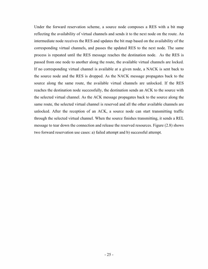
- 25 -
Under the forward reservation scheme, a source node composes a RES with a bit map
reflecting the availability of virtual channels and sends it to the next node on the route. An
intermediate node receives the RES and updates the bit map based on the availability of the
corresponding virtual channels, and passes the updated RES to the next node. The same
process is repeated until the RES message reaches the destination node. As the RES is
passed from one node to another along the route, the available virtual channels are locked.
If no corresponding virtual channel is available at a given node, a NACK is sent back to
the source node and the RES is dropped. As the NACK message propagates back to the
source along the same route, the available virtual channels are unlocked. If the RES
reaches the destination node successfully, the destination sends an ACK to the source with
the selected virtual channel. As the ACK message propagates back to the source along the
same route, the selected virtual channel is reserved and all the other available channels are
unlocked. After the reception of an ACK, a source node can start transmitting traffic
through the selected virtual channel. When the source finishes transmitting, it sends a REL
message to tear down the connection and release the reserved resources. Figure (2.8) shows
two forward reservation use cases: a) failed attempt and b) successful attempt.

- 26 -
Figure 2.8: Forward reservation use cases
The authors describe 4 variations of the forward reservation protocol: aggressive forward
reservation with dropping (AFD), aggressive forward reservation with holding (AFH),
conservative forward reservation with dropping (CFD), conservative forward reservation
with holding (CFH). A scheme with a holding characteristic allows an intermediate node to
hold a failing RES message for a pre-defined period of time; otherwise, it has a dropping
characteristic. If some corresponding virtual channels become available within the pre-
defined holding time, the RES is updated and sent forward; otherwise, a NACK is sent
backward. On the other hand, an aggressive scheme requires that intermediate nodes lock
all the available virtual channels along the path of a RES message. In this case, success is
guaranteed if any virtual channel is identified. Alternatively, the conservative scheme
Source DestinationIntermediate Source Destination
RES
FAIL/NACK
Retransmit time
RES
ACK
REL
send data
(a) (b)
- 27 -
requires that intermediate nodes lock a single virtual channel. In this case, success is
guaranteed only if the designated virtual channel is available on all links.
With backward reservation protocols, five types of messages are used:
• Probe Message (PROB): it is an information gathering message that has a bit map
reflecting the availability of virtual channels (i.e. wavelengths or time slots).
• Reservation Message (RES): It is similar to the RES message described in the
forwarding scheme, except that it travels backward as it is described next.
• Fail message (FAIL): It is used to unlock virtual channels locked by RES in case of
failure in establishing a connection.
• Negative Acknowledgment Message (NACK): It is used to inform the source node
of a reservation failure.
• Release Message (REL): It is a connection release request that includes the
connection identifier.
Under a backward reservation scheme, a source node composes a PROB with a bit map
reflecting the availability of virtual channels and sends it to the next node on the route. An
intermediate node receives the PROB and updates the bit map based on the availability of
the corresponding virtual channels, and passes the updated PROB to the next node. The
same process is repeated until the PROB message reaches the destination node. Unlike the
forward reservation scheme, the available virtual channels are not locked as the PROB is
passed from one node to another along the route. If no corresponding virtual channel is
available at a given node, a NACK is sent back to the source node and the PROB is
dropped. If the PROB reaches the destination successfully, the destination node sends a
RES to the source with a bit map reflecting a selected subset of the PROB bit map. As the
RES message propagates back to the source along the same route, each intermediate node
checks the availability of selected virtual channels, updates the RES bit map accordingly,
and locks the available ones. If no virtual channel is available at a given point, a NACK is
sent to the source and a FAIL is sent to the destination to unlock the already locked
resourced. The same process is repeated until the RES message reaches the source node. If
the RES reaches the source node successfully, the source sends an ACK to the destination
with the selected virtual channel. As the ACK message propagates to the destination along

- 28 -
the same route, the selected virtual channel is reserved and all the other available channels
are unlocked. Note that a source node can start transmitting traffic through the selected
virtual channel right after the reception of an ACK. When the source finishes transmitting,
it sends a REL message to tear down the connection and release the reserved resources.
Figure (2.9) shows three backward reservation use cases: a) failed attempt during a probing
pass, b) failed attempt during a reservation pass and c) successful attempt.

- 29 -
Figure 2.9: Backward reservation use case
Source DestinationIntermediate
PROB
NACK
Retransmit time
(a)
Source Destination
PROB
Source DestinationIntermediate
PROB
NACK
Retransmit time
(b)
PROB
RES
FAIL
PROB
ACK
RES
REL
send data
(c)

- 30 -
Similar to the variation of the forward reservation, the authors describe 4 variations of the
backward reservation protocol: aggressive backward reservation with dropping (ABD),
aggressive backward reservation with holding (ABH), conservative backward reservation
with dropping (CBD), conservative backward reservation with holding (CBH). A
backward scheme with a holding characteristic shares similar functionalities with its
counterpart in the forward reservation side; however, it allows an intermediate node to hold
only a failing RES message, but not a PROB, for a pre-defined period of time; otherwise it
has a dropping characteristic. In addition, in case of failure, a NACK is sent to the source;
and, a FAIL is sent to the destination. Similarly, the aggressive and conservative
approaches resemble their forward reservation counterparts, but in the opposite direction.
Note that if a conservative reservation scheme is adopted, the ACK message is not
necessary.
As a result of their study, Yuan et al. reported that the conservative schemes outperformed
the aggressive scheme; and, the backward schemes outperformed the forward schemes
under the same aggressiveness level. They noted that the conservative forward scheme has
higher throughput than the aggressive backward scheme. In addition, when the wavelength
number is reasonably large, the holding characteristic improves the performance for all
schemes except for the conservative forward scheme. They also found that the message
size has a large effect on the performance of a protocol. The message size reflects the
amount of information loaded on a given message. For example, the size of a RES message
depends on the size of the associated bit map reflecting the virtual channel availabilities;
i.e., the larger the number of virtual channels is, the higher the message size gets. Using
small messages, better performance was noticed with conservative schemes in comparison
with their aggressive counterparts. On the other hand, large messages boosted the
performance of backward schemes in comparison with their forward scheme counterparts.
Generally, a backward scheme always outperformed a forward scheme when all other
characteristics are alike.
In [Yuan1997], Yuan et al. repeated the same study in their previous work [Yuan1996] but
with additional characteristics such as network size, re-transmission rate and control

- 31 -
network speed. They reported that the backward schemes provided better performance
when the message size is small and when the network size is large. When the message size
is large or the network size is small, all the protocols showed similar performance. The
authors added: “The speed of the control network affects the performance of the protocols
greatly.” [Yuan1996] As another variation, the author considered an optimized
conservative approach. They reported that choosing an optimal virtual channel bit map,
covering a subset of the network channels, in the RES message improved performance by
about 100% in the forward reservation schemes and 25% in the backward schemes.
In [Mei1997], Mei and Qiao presented a similar study to what Yuan et al. did in
[Yuan1996], but used different nomenclatures to describe the various schemes. They
reported similar results in general. The major differentiators in their study are the
consideration of Path Multiplexing (PM) versus Link Multiplexing (LM), and primary path
versus alternative paths routing with CBH (CBH-PRIME and CBH-ALT). PM denotes the
usage of the same wavelength across the entire path. LM denotes the possibility of using
different wavelengths across the path (i.e. wavelength conversion) [Qiao1997]. They
showed that CBH-ALT with LM improves the throughput over the best forward
reservation scheme under LM (which is CFD) by 10%; while CBH-PRIME did not provide
a significant improvement. On the other hand, CBH-PRIME with PM improved throughput
over the best forward reservation scheme under PM (which is AFD) by 10%; while CBH-
ALT did not improve the performance further.
In [Hafid2005b], Hafid et al. extended the advance reservation scheme in [Hafid2005a] to
serve inter-domain networks. In their solution, each network has a central Advance
Reservation Manager (ARM) responsible for the internal reservation process. For inter-
domain scheduling, when every network’s ARM handles the internal scheduling task, it
appends its proposal to a list and forwards it to the next ARM on the route. At the
destination ARM, the resulting list of proposals is sent backward to the source ARM. The
source ARM forwards the list to the user in order to select the best proposal. After
selecting a proposal, a confirmation message is propagated forward to the destination in
order to reserve the appropriate resources. The authors did not evaluate the inter-ARM

- 32 -
signaling in terms of bandwidth utilization and efficiency. However, we can easily see that
the proposed signaling scheme is bandwidth inefficient due to its three ways messaging,
and the growing list of proposals appended to the message. Figure (2.10) shows four
ARMs communication scenarios: a) successful reservation, b) negotiation failure, c) failure
due to insufficient resources at the destination, and d) failure due to insufficient resources
at an intermediate ARM.
Figure 2.10: ARM communication use cases
Source ARM
Destination ARM
Transit ARM
Setup
(a) (b)
Setup
Confirm Confirm
Commit
Commit
Source ARM
Destination ARM
Transit ARM
SetupSetup
Confirm
Commit
Commit
Uncommit
Source ARM
Destination ARM
Transit ARM
Setup
(c) (d)
Setup
Reject
Reject
Source ARM
Transit ARM
SetupSetup
Commit
Reject
Destination ARM

- 33 -
In [Yang2007a], Yang et al. compares the performance of four distributed RWTA
algorithms in a bidirectional ring network. In each algorithm, they only vary the
wavelength allocation scheme and use shortest path routing and first-fit time slot
reservation. The four wavelength allocation schemes that they utilized are: the First Fit,
Random, Most Loaded and Least Loaded wavelength. They assume no global knowledge
in the network, where each node only has local knowledge about the resources on its
outgoing links. To achieve bandwidth reservation in this environment, backward
reservation is required. Essential information about resources at every node along the path
must be collected in a forward message travelling from the source to the destination. When
the destination receives this forward travelling message, it chooses the appropriate
resources and sends a backward message towards the source. It is the typical backward
reservation approach described earlier in this section.
In [Yang2007b], Yang et al, investigated the forward reservation scheme assuming global
knowledge at each node. Due to the need for extensive signaling to maintain this global
knowledge, the authors resorted to the well-known technique of periodic resource update
[Shaikh2001, Shen2004, Shen2006]. They studied the effect of varying the update interval
under two different reservation schemes, First Fit and Random. They found that the
Random scheme outperformed the First Fit at all levels of periodic updates. They justify
this observation by saying: “FF tends to pack wavelengths/time slots according to a fixed
order. When traffic load is very light, the stale global information is more likely to cause
FF to make incorrect routing, wavelength and time slot assignment decisions than RR,
which in turn may cause more blocking for FF than RR.”
2.5. Multi-Protocol Label Switching Over the years, Multi-Protocol Label Switching (MPLS) [RFC3031] has evolved to be the
dominant packet-switched protocol in the telecommunication field. From an OSI
perspective, MPLS fits between the layer 2 (Data Link) and layer 3 (Network). An MPLS
network serves as a transparent medium for any traffic type, such as IP, ATM, Frame

- 34 -
Relay and Ethernet. With the insertion of a 4-bytes shim header, which includes a label,
any traffic segment, regardless of its origin and size, can be routed through an MPLS
network towards its destination. In this sense, MPLS wins over ATM when it comes to
bandwidth efficiency and adaptability since ATM uses a 5-bytes header for every 48 bytes
of data. In addition, exhaustive segmentation and assembly are required to adapt to other
protocols. On the other hand, MPLS is a perfect solution for IP-based traffic as it helps in
carrying IP traffic past the IP network boundaries in a feasible way. It just inserts the
relatively small shim header without the need to dissect the routed IP packet.
2.5.1. MPLS Header The MPLS shim header is made of the following parts, as shown in Figure (2.11):
- Label: 20 bits carrying a label value.
- CoS: 3 bits defining Quality of service parameters.
- S (Stack Field): 1 bit defining that the current label is the last in the stack
- TTL: 8 bits reflecting the time to live
Figure 2.11: MPLS Header
2.5.2. Resource Allocation in MPLS An MPLS network is made of Labeled Edge Routers (LER) and Labeled Switch Routers
(LSR). The LER nodes are the first and last nodes through which a traffic segment should
pass when routed in an MPLS network. These are the entry and exit points where the label
Label CoS S TTL
20 bits 3 bits 8 bits
1 bit

- 35 -
is inserted into, and stripped from, the traffic segment. On the other hand, the LSR nodes
forward the segment to its destination based on the carried label. To route traffic over an
MPLS network, a Labeled Switched Path (LSP) must be established between two LER
points, and might pass through several LSR nodes depending on the routing and quality of
service parameters. The ingress LER initiates a label request message and forwards it to the
egress LER through the appropriate route. Upon receipt of the request, the egress LER
returns a label via a label mapping message. Each individual LSR along the reverse route
updates its forwarding table accordingly and redefine the label for the upstream LSR or
LER. Figure (2.12) represents a graphical example of the reservation process. The Label
Distribution Protocol (LDP) [RFC3036, RFC3212] and the Resource Reservation Protocol
(RSVP) [RFC2205, RFC3209] are the most common protocols that are adopted in MPLS
for LSP reservation.
Figure 2.12: MPLS reservation process
2.5.3. Resource Update in MPLS In MPLS, each node has a database keeping track of various network resource information
and status. The nodes exchange resource information via update messages based on the
Open Shortest Path First (OSPF) [RFC2328, RFC3630] or Intermediate System to
Intermediate System (IS-IS) protocols [RFC1629]. Status update in MPLS happens on a
periodic basis rather than immediately after a change, usually at a interval between 5 sec
and 30 min [RFC2328, RFC4316]. Hence, the nodal database might not reflect the true
status of a network in the period between two update sessions. However, the benefits of
saving the bandwidth overhead and the signaling cost associated with exhaustive
Ingress LER - A
Ingress LER - D
LSR - B LSR - C
Label Request
Label Mapping (label 100)
Label Mapping (label 142)
Label Mapping (label 76)
Label Request Label Request

- 36 -
immediate updates justify the inconvenience of having a slightly outdated database.
2.5.4. Generalized MPLS To employ MPLS in an optical network, some enhancements were necessary to the MPLS
protocol suites. The RSVP and LDP protocol were adjusted to support signaling and
creation of optical channels [RFC4974, RFC3472]. In addition, OSPF and IS-IS were
extended to carry updates on optical resources status such as bandwidth availability and
local constraints [RFC4203, RFC4205]. These enhancements were the essence behind the
emergence of the Generalized MPLS (GMPLS) [Banerjee2001, Lang2004, RFC3471],
which is meant to apply MPLS in optical networks. With GMPLS, the label or LSP can be
a time slot, a wavelength, or a full fiber. In addition, hierarchical LSPs are supported in the
context of GMPLS. A hierarchy of LSPs is formed when one LSP is tunneled inside
another existing LSP. For example, a fiber-level LSP could exist between two nodes and
yet could be carrying different wavelength-level LSPs serving various source-destination
node pairs. See Figure (2.13) for a graphical illustration.
Figure 2.13: Hierarchical LSPs in GMPLS
Fiber level LSP
Wavelength level LSP
Timeslot level LSP
LSR

- 37 -
3. Least Constraining Slot Allocation
3.1. Problem Definition As discussed in the review chapter, some research papers [Chen2004, Liew2003,
Siew2006, Wen2005, Zang1999, Zang2000] assumed time slot boundaries synchronization
instead of frame. However, that comes with the price of loosing frame alignment, and
hence the benefit of adopting wavelength allocation schemes as possible solutions for the
time slot reservation problem. Thus, finding an effective time slot reservation scheme in an
optical network, where transmission is synchronized on slot and not frame boundaries,
becomes a vital question.
In this chapter, we propose a novel time slot reservation schemes in all-optical TDM mesh
network without buffers at nodes, where transmission is synchronized on slot boundaries.
With the introduction of this scheme, we aim to reduce call blocking to a close to optimum
rate achieved with buffering. We consider that the reservation of a slot imposes constraint
on the network measured by the number of transmission channels on the fixed routes that
might use the slot at a given point in time. The scheme selects the least constraining slots
on the route, hence the name “least constraining” (LC) slot. We use the FF approach with
full time slot interchanging capability as a benchmark to measure our results. It has been
proven that employing full wavelength interchanging yields optimum results with fixed
routing [Zeineddine1998]. This is true because blocking would not occur unless one of the
links along the fixed route is saturated. In addition, we compare the performance of the LC
approach to the LL approach in a multi-fiber environment. We also investigate how LC
behaves in a star network synchronized on slot boundaries.

- 38 -
3.2. LC Allocation approach
3.2.1. Basic Concepts Before describing the basic steps of the LC approach, we should clarify the nomenclature
used in this chapter to provide a better understanding of the presented concepts. Route,
route-slot and link-slot are essential concepts used in describing the LC approach.
Assuming fixed alternative routing, a network route is a predetermined series of
unidirectional links interconnected through intermediate nodes from a given source node to
a given destination node. We say that two routes intersect if they have at least one link in
common. A node transmits data into a link in the form of repeating frames of N equal time
slots. Due to the link propagation delay, frame alignment is not preserved along the route.
However, slot boundary synchronization is assumed. Considering link AB from node A to
node B, data transmitted during a given time slot at egress node A might be received during
a different time slot at ingress node B. Thus, a time slot is better identified with reference
to a link; we use the term link-slot ABx to describe time slot x on link AB. There is no need
to mention the corresponding wavelength since only one wavelength plane is considered in
this study; basically, the LC approach is designed to operate at a sub-wavelength level and
is independent of the number of employed wavelengths. Formally speaking, a link-slot is a
time slot on a link with reference to the frame of its egress node. In general, a transmitted
data from source node S to destination node D travels through different links along a fixed
route, and hence occupies a series of different link-slots. For instance, if A and B are two
intermediate nodes between S and D, a series of link-slots would be described as SAx ABy
BDz. Knowing the delay of each link, an intermediate link-slot UVj corresponds to a source
link-slot SAi according to the general rule ( ) Nmoddij SU+= , where dSU is the total delay
of all links from node S to node U. Thus, knowing the fixed route between a source-
destination pair and all associated link delays, one can easily derive the entire series of
link-slots when given a starting link-slot. In this case, we can describe the series SAx ABy

- 39 -
BDz in a simple notation xSD , which we call a route-slot. The upper bar is essential to
differentiate between link-slot and route-slot. A route-slot xSD is considered available if all
its constituent link-slots are available; otherwise, xSD is unavailable. In a single fiber
environment, a link-slot is available if it is not reserved. On the other hand, in a multi-fiber
case, a link-slot is available if it is free at least on one of the link fibers. To make our
approach generic enough, we develop it based on a multi-fiber environment, and apply it to
a single-fiber network as a special case.
The exercise of allocating resources, for a communication request, from node S to D is to
find and reserve an available route-slot xSD along a given fixed route.
3.2.2. Basic Definitions
3.2.2.1. Resource Availabilities
If a link-slot XYj is part of a route-slot iSD , we write:
ij SDinXY , which implies that ( ) Nmoddij SX+= . (3.1)
Considering M fibers per link, we define the link-slot availabilityjXYΑ , an integer between
0 and M, to be the number of fibers on which XYj is free. If jXYΑ is equal to zero, then XYj
is unavailable. Furthermore, we define the availability iSD
Α of a route-slot to be equal to
the minimum availabilityjXYΑ among its constituent link-slots,
( )j
iji XY
SDinXYSDMIN ΑΑ = . (3.2)

- 40 -
A route-slot’s availability could be identical to the availabilities of several constituent link-
slots. This could happen when several link-slots have the same minimum availability. We
define the count of link-slots who share the same availability with their container route-slot
as the availability-matching-count:
=≠
== baif,1
baif,0)b,a(Equalwhere),(EqualE
ij
jiiSDinXY
XYSDSDΑΑ (3.3)
3.2.2.2. Intersecting Route-Slot Sets
Knowing the set of fixed alternative routes that can be used for each source-destination
pair, we derive the set Ω of all possible route-slots in the network. We define jXYΩ to be a
subset of Ω consisting of all route-slots that contain link-slot XYj.
ijiXY SDinXY|SDj
ΩΩ ∈= . (3.4)
We further define jXY'Ω to be a subset of
jXYΩ consisting of all route-slots whose
availabilities are equal tojXYΑ .
jijj XYSDXYiXY |SD' ΑΑΩΩ =∈= . (3.5)
The purpose of jXY'Ω is to identify all route-slots whose availabilities are decremented
when the link-slot XYi is reserved.
In addition, we define jXYΩ ′′ to be a subset of
jXY'Ω consisting of all route-slots whose
availability-matching-counts are equal to 1:

- 41 -
1E|SDijj SDXYiXY =′∈=′′ ΩΩ (3.6)
The purpose of jXYΩ ′′ is to identify all route-slots whose availabilities are incremented when
the link-slot XYi is released.
3.2.2.3. Resource Constraint
We designate the constraint of link-slot XYi to be the sum of the availabilities of all route-
slots belonging tojXYΩ .
∈
=jXYi
ij
SDSDXYC
Ω
Α . (3.7)
In a single fiber environment, iSD
Α becomes a binary variable showing whether the route-
slot is available (1) or not (0); and hence, jXYC would reflect the number of available
route-slots containing XYj. In other words, it indicates the number of routes that can
potentially use the designated link-slot.
Last, we define the constraint of a route-slot to be equal to the total constraint of all its
constituent link-slots:
=ij
jiSDinXY
XYSDCC . (3.8)
To clearly understand the relationship between the constraint of a route-slot and the
availabilities of the intersecting route-slots, we expand Equation 3.8 with 3.7:
∈
=ij jXYn
ni
SDinXY ZPZPSD
CΩ
Α (3.9)
- 42 -
In addition, to describe the relationship between the constraint of a route-slot and the link-
slots that define the availabilities of the intersecting route-slots, we expand further with
Equation 3.2, we get:
( ) ∈
=ij jXYn
jnj
i
SDinXY ZPUV
ZPinUVSDMINC
Ω
Α (3.10)
3.2.3. Allocation Principle Equation 3.7 shows that the constraint of a route-slot reflects the total availability of all
route-slots that intersects with it in one of its links. Thus, the route-slot’s constraint is an
indicator of the number of available route-slots that could use one of its constituent link-
slots. It is evident that reserving a route-slot which has the least impact on other available
route-slots keeps more available resources in the network, hence improves the blocking
rate for subsequent communication requests. Here, the impact on other available route-slots
is measured by the constraint. Thus, the route-slot that has the lowest constraint iSD
C would
be the best choice on a given route between S and D. In this case, only a minimal number
of route-slots in the network could become unavailable when serving a given call.
3.2.4. Constraint Update After identifying the best route-slot, all constituent link-slots are reserved. Consequently,
the constraint of each link-slot in each route-slot in iXY'Ω is modified according to the
algorithm, shown in Figure (3.1).

- 43 -
Figure 3.1: Constraint update algorithm
By definition (4), jXY'Ω contains all route-slots whose availabilities are decremented due
to a reservation of XYj. For instance, when reserving XYj in a single fiber environment, all
route-slots in jXY'Ω become unavailable, and accordingly, their availabilities flip from 1 to
0. Therefore, the constraint of their constituent link-slots must be decremented since a link-
slot constraint is the sum of the availability of the intersecting route-slots.
Finally, a similar algorithm is repeated when freeing resources, but the set Ω′′ is used
instead of Ω′ , and the constraints are increased instead of decreased. See Figure (3.2). We
use Ω′′ because we are only interested in the route-slots whose availabilities will be
increased after releasing the corresponding link slot. If a route-slot has multiple link-slots
with the same minimum availability, increasing the availability in one of these link-slots
should not affect the route-slot availability. Route-slot availability should increase only if
the released link-slot is the only constituent link-slot that has the minimum availability.
foreach ij SDinXY do 1C:C
jj XYXY -=
foreach jXYn 'RT Ω∈ do
if in SDRT ≠
foreach nk RTinUV do
1C:Ckk UVUV -=
ReserveLinkSlot(XYj)

- 44 -
Figure 3.2: Constraint update algorithm
3.2.5. Illustrative Example In the network of Figure (3.3), a circle defines a node, and an arrow represents a
unidirectional single fiber link during a particular link-slot. Next to each arrow is an
underlined delay value in slot unit. The dashed area represents network segments where no
communication is possible from/to EG10 and GF5 due to unavailability of matching link-
slots.
Considering a transmission request from node E to node F, we should find an available
route-slot that has the lowest constraint on route EGF. We assume 3 available route-slots
were identified, 1082 EFand,EF,EF . Let us start with measuring the constraint of 10EF
based on the logistics of Figure (3.3). By definition (6), the constraint of a route-slot is
equal to the total constraint of all its constituent slots, 51010
GFEGEF CCC += . Assuming a
single fiber environment, we would benefit from identifying 10EG'Ω to get the constraint of
EG10; 101066447733EG EG,EF,DG,DF,CG,CF,BG,BF,AG,AF'10
=Ω . Since the
availabilities are either 0 or 1 in a single fiber network, a route-slot being in 10EG'Ω means
that its availability is 1. Thus, 10EGC is given by ( )
10EG'Size Ω , which is 10. Similarly for
foreach ij SDinXY do 1C:C
kk UVUV +=
foreach jXYnRT Ω ′′∈ do
if in SDRT ≠
foreach nk RTinUV do
1C:Ckk UVUV +=
FreeLinkSlot(XYj)

- 45 -
GF5, we find 95106473GF HF,GF,EF,DF,CF,BF,AF'5
=Ω and 7C5GF = ;
and hence, 17710C10EF =+= . Repeating the same process for
2EF and8EF , which have
different logistics not shown in Figure (3.3), we may find 21C2EF = and 19C
8EF = . As a
result, 10EF has the lowest constraint and is chosen for reservation. We reserve the
constituent link-slots EG10 and GF5, and decrement the constraint of each link-slot found in
each route-slot in 10EG'Ω and
5GF'Ω , except for 10EF .
Figure 3.3: A route-slot (10EF ) and its related link-slots
4
5
4
3
4
3
C
A
B
E
G
D
H
F
AB3
CB4
BE7
DE6
EG10
GF5
6
HG9

- 46 -
3.3. Simulation Results In this section, we compare the performance of the LC approach against the FF scheme and
FF with OTSI in a single fibre network, and also with LL in a multi-fibre network. In
addition, we determine its effectiveness in ring and star topologies.
3.3.1. Simulation The simulation experiments are based on the 14-node 21-link NSFNET network topology
shown in Figure (3.4). We also used a 14-node ring and star topologies as shown in Figures
(3.5) and (3.6). A link between two nodes consists of dual unidirectional fibres with a fixed
capacity of 10 time slot channels per fibre. Fixed k-alternative paths routing is used to
derive paths between all source destination pairs [Sukhni2008], where k in our simulation
was defaulted to 1 unless noted otherwise. The first path between a source destination pair
is the shortest; the nth one is the shortest path that does not have any link-intersection with
the other n-1 paths. Each path serves up to 10 concurrent connections at the granularity of a
transmission channel, i.e. one time slot per link along the path. Each simulation is repeated
for 30 runs; each run goes until 100,000 calls are attempted. Calls arrive according to a
Poisson process, and lasts for an exponentially distributed period. The simulation results
concerning blocking probabilities have confidence intervals similar to those shown in
Figure 3.7 where the 95% confidence intervals are plotted.

- 47 -
Figure 3.4: NSFNET topology
Figure 3.5: A 14-node ring topology
1
2
3
4 5
7
8
6 10
11
9 12
14
13
1
2
3 4 5
7
8
6
10
11
9
12
14
13

- 48 -
Figure 3.6: A 14-node star topology
We study our scheme under two different traffic distributions among source-destination
pairs, uniform and non-uniform. In the uniform traffic case, every pair is chosen at random
with equal constraint and hence having the same traffic load in Erlang (mean arrival rate ×
mean holding time). In the non-uniform case, source-destination pairs have different
constraints to achieve non-uniform traffic distribution. Traffic quotas are non-uniformly
distributed among 8 random groups of source-destination pairs. Each one of these groups is
assigned a different percentage of the network traffic load. For example, assume that 3% of
random SD pairs are assigned 30% of the load; this translates, in a network of 200 SD node
pairs, to 6 random SD pairs each having 5 percent chance of generating traffic calls. Here
is the table that the simulation follows in randomly distributing the traffic load in the
network:
SD Node Group
(% of total SD pairs)
Traffic Load
(% of network load)
3 30
3 20
5 15
10 10
1
2
3
4 5
7
8
6
10
11
9
12
14
13
X

- 49 -
10 08
20 07
20 06
29 04
Tab. 3.1: Non-Uniform Traffic Distribution Map
3.3.2. Observations Figure (3.7) shows the improvement in blocking probability that the LC approach achieves
in comparison to the FF approach. The LC approach, under uniform traffic distribution,
provides a performance gain almost identical to the case of using optical time slot
interchangers with the FF approach. It is worthwhile noting that with the use of
interchangers all blocked calls, in our simulation, happened due to link saturation along the
fixed route. Hence, the performance results of employing OTSIs are the optimum any
reservation scheme can achieve under a fixed routing approach. Thus, the LC approach
achieves close to optimum performance.

- 50 -
1.E-06
1.E-05
1.E-04
1.E-03
1.E-02
1.E-01
1.E+00
30.0 35.0 40.0 45.0 50.0
load (Erlang)B
lock
ing
prob
abilit
y
FF FF+OTSI LC
Figure 3.7: LC vs. FF with uniform traffic
Figure (3.8) reflects the results of applying non-uniform traffic distribution among source
destination node pairs. The blocking rate in all cases was higher than what was achieved
under uniform traffic distribution. However, the LC approach maintained its optimal
performance as compared to the FF approach with OTSI. The charts show that LC and FF
with OTSI yielded identical performance. The reason for this is the randomness in
distributing calls among source destination pairs at each simulation run. Considering two
routes under similar loads, the route that intersects with more other routes would make
more impact on network performance. This route is considered more critical than the other.
Take for example one simulation run for the FF approach with OTSI. If a large number of
critical routes get a high percentage of the load, the performance tends to go below
average. Now, consider a simulation run with the LC approach. If a similar number of less
critical routes get the same high load percentage, performance tends to be above average.

- 51 -
Due to random load distributions, simulation runs produced numbers below and above
average in both cases, LC and FF with OTSI. However, after 30 runs of each case,
performance averages out to the same level as shown in Figure (3.8).
1.E-06
1.E-05
1.E-04
1.E-03
1.E-02
1.E-01
1.E+00
25.0 30.0 35.0 40.0 45.0
load (Erlang)
Blo
ckin
g pr
obab
ility
FF FF+OTSI LC
Figure 3.8: LC vs FF with non-uniform traffic
Figure (3.9) shows that the LC approach provided better performance results than the LL
approach when applied to a multi-fibers network consisting of 3 fibers per link. It
outperformed LL at every load level. In addition, the LC approach can be applied to single
and multi-fiber environments; on the other hand, the LL approach collapses to an FF
approach in single fiber networks, and hence loses its benefit.

- 52 -
1.E-06
1.E-05
1.E-04
1.E-03
1.E-02
1.E-01
1.E+00
150.0 200.0 250.0 300.0 350.0
load (Erlang)B
lock
ing
prob
abili
ty
FF LL LC
Figure 3.9: Comparing LC to LL in multi-fiber networks (3 fibers per link)
In all the simulation runs, the default number of routes per source-destination pairs was
always 1. Figure (3.10) represents the performance of the LC approach when 2 alternative
routes are employed. It shows that the same performance trend is achieved regardless of
the number of alternative routes adopted between a source-destination pair. In fact,
incrementing the number of routes has no effect other than increasing the size of Ω, and
hence having larger resource constraints.

- 53 -
1.E-06
1.E-05
1.E-04
1.E-03
1.E-02
1.E-01
1.E+00
50.0 60.0 70.0 80.0 90.0 110.0
load (Erlang)
Blo
ckin
g pr
obab
ility
FF FF+OTSI LC
Figure 3.10: LC vs FF with 2 alternative-paths routing
Figure (3.11) shows the performance of the LC approach in a 14-node ring network
topology. The performance trend resembles the results of the mesh network shown in
Figure (3.7). The difference in blocking rate between Figure (3.11) and (3.7) for the same
load level is due to the reduced number of links between the ring and mesh topologies. A
14-node ring has 13 links compared to the 21-link NSFNET topology. In addition, the
average hop count is 3.8 in the 14-node ring compared to 2.3 in the NSFNET topology.

- 54 -
1.E-06
1.E-05
1.E-04
1.E-03
1.E-02
1.E-01
1.E+00
15.0 20.0 25.0 30.0 35.0 40.0
load (Erlang)
Blo
ckin
g pr
obab
ility
FF FF+OTSI LC
Figure 3.11: LC performance in 14-node ring network
Figure (3.12) shows the performance of the LC approach in a star network topology. It
provides identical results to the FF approach. This result is expected since all links in a star
have the same number of intersecting 2-hops routes; hence, all link-slot constraints were
initially equal. In addition, when a reservation is made on a link-slot, corresponding link-
slots in all other links get equally updated. Thus, the LC approach collapses to an FF
approach in a star topology since the constraint scheme would have no impact.

- 55 -
1.E-06
1.E-05
1.E-04
1.E-03
1.E-02
1.E-01
1.E+00
30.0 35.0 40.0 45.0 50.0
load (Erlang)B
lock
ing
prob
abili
ty
FF LC
Figure 3.12: Measuring LC in a star network
Figure (3.13) shows two charts of the LC approach performance with non-uniform traffic
distribution in NSF network. One of the charts represents the normal LC approach; and, the
other shows the results of a modified version of the LC approach where the constraint of a
link-slot is based on the intersecting route-slots availabilities multiplied by their
corresponding routes load percentage ρSD according to the following Equation:
( )∈
×=jXYi
ij
SDSDSDXYC
Ω
ρΑ . For example with a non-uniform traffic distribution, if route
SD serves 5 percent of the network traffic load, ρSD is then equal to 5. The charts clearly
shows that considering the traffic loads of interesting routes when calculating resource
constraints has no impact on the performance of the LC approach. In that sense, we say
that the resource constraint in LC approach is load independent. As an elaboration, all link-

- 56 -
slots on a given link are equally loaded although the load distribution in the network is not
uniform. The average load for a link-slot XYj is XY
SDSD
XY NXY
j Λ×=
Λ∈
ρρ , where ΛXY is the set of
routes passing through link XY. Therefore, including the load in the link-slot constraint
calculation does not add any value.
1.E-06
1.E-05
1.E-04
1.E-03
1.E-02
1.E-01
1.E+00
25.0 30.0 35.0 40.0 45.0 50.0
load (Erlang)
Blo
ckin
g pr
obab
ility
FF LC with load factor LC
Figure 3.13: LC performance after factoring the load in the resource constraints
3.4. Analytical Discussion In this section, we develop an equation for the blocking probability of the LC approach as a
factor of the blocking probability of the FF approach. Our intention behind this informal

- 57 -
analysis is to add some clarity and assurance to the simulation results. It is imperative to
say that this analysis is approximate. Most of the derived equations are approximations
based on the assumption of uniform traffic distributions between all pairs of nodes and of a
network architecture where all links are equally loaded. Over the course of our analytical
discussion, we rely on the following basic definitions:
Symbol Description
n Number of nodes
l Number of links
f Number of fibers per link
t Number of time slots per frame
λ Poisson arrival mean
σ Average holding time
n
ld =
Average nodal degree
(number of links / number of nodes)
d2
nh =
Average hops count
(max hops count / 2)
( )l
h1nnr
×−×= Average number of intersecting routes per link
(sum of link counts in all routes / number of links)
λ
σ=e Average number of active connections
(average holding / mean arrival)
ftl
he
××
×=μ
Load factor
(number of used time slots / total number of time slots)
Tab. 3.1: Analysis Symbols
Knowing the number of reserved connections (given by e) in the network, the average link-
slot constraint can be calculated as follows:

- 58 -
updmaxXY CCCj
−= (3.11)
where Cmax is the maximum constraint value a link-slot can have:
frCmax ×= (3.12)
and Cupd is the average reduction of the constraint due to updates resulting from the
reservation of e connections:
tl
KrheC
2
upd ××××= (3.13)
The parameter K represents the probability of a route-slot’s availability being equal to the
reserved link-slot’s availability. Note that a link-slot reservation should affect an
intersecting route-slot’s availability only if they have the same availability. In this case, the
constraints of the constituent link-slots should be updated. A route-slot’s availability is
equal to a link-slot’s availability if this link-slot has the lowest availability among all
constituent link-slots. Thus, K is equal to the probability of a link-slot’s availability being
less than or equal to all link-slot’s availabilities in a route of h hops.
( )[ ] 1hAA
xUVjXYPK −
≤= (3.14)
Knowing the availability range [0. .f] and assuming that the availability of a link-slot can
be any value in that range with equal probability, the probability that a link-slot’s
availability is less or equal than the availability of another link-slot can be approximated
as:

- 59 -
( ) ( ) ( )1f2
2f
1f
zP
2
1f
1zAA
xUVjXY +×+=
+=
+
=≤ (3.15)
By definition, the link-slot constraint is the sum of the availabilities of all route-slots that
intersect in it. Therefore, it indicates the number of possible connections that get blocked
should the link-slot become unavailable. In other words, reserving a link-slot XYi, having
1AjXY = , would consequently block an average of
jXYC possible connections. Thus, the
number of blocked connections, when the link-slot gets unavailable, is equal to the link-
slot’s constraint at the reservation time. Let jXYB be the average number of blocked
connections as a result of consuming the last availability on a link-slot. If υ is the average
number of link-slots that are unavailable in a uniformly loaded network, the network
blocking probability can be described as follows:
ftl
BP jXY
××
×=
υ (3.16)
If ( )FFP and ( )LCP are the blocking probabilities related to the FF and LC approaches,
respectively, we derive:
( ) ( )FFFFXY
LCXY
LC PB
BP
j
j ×= (3.17)
With the FF approach, there is no mandate to select the least constraining route-slot during
the allocation process, as in the LC case; selection is rather arbitrary. Thus, the average
number of blocked connections when reserving XYj FFXY j
B tends to be equal to the average
link-slot constraint described in Equation (3.11). On the other hand, the LC approach

- 60 -
always favors the least constraining route-slots; and hence, LCXY j
B tends to be below average
according to the following formula:
10where,CBjj
XYLCXY ≤<×= δδ (3.18)
and, consequently
( ) ( ) 10where,PP FFLC ≤<×= δδ (3.19)
To get an approximation of LCXY j
B , we need to understand the distribution of the constraint
values in the network. A link-slot constraint can be between 0 and maxC . Figure (3.14)
shows the distribution trend of constraint values amongst the link-slots in the network.
Each chart represents the percentage trend of link-slots that have low, medium, and high
constraints under a specific load level. In a non-loaded network, all link-slot constraints are
equal to maxC ; i.e. 100% of link-slots have high constraints. We know that the constraint
of a reserved link-slots is reduced by Kr × ; and consequently, the constraint of
( ) Kr1h ××− updated link-slots is reduced by 1. Thus, the constraint of a reserved link-
slot is reduced at a much greater rate than an updated link-slot. In a low loaded multi-fiber
network, the number of reserved link-slots given by he × is low; however, the number of
updated link-slots given by ( ) Kr1he ××−× is relatively high. Thus, the percentage of
link-slots having low constraints is low, and the percentage of link-slots having medium
constraints is relatively higher. This trend is different in a single-fiber network due to the
narrower range of constraint values, where rCmax = . The average reduction rate in a
single-fiber network is updC
r; while this rate is
updC
fr × in the multi-fiber case. In addition,
a reserved link-slot in a single-fiber network has zero-constraint since it has zero-
availability which eventually blocks all intersecting route-slots. Thus, the percentage of
link-slots having low constraints is much higher than those with medium constraints in a

- 61 -
low loaded single-fiber network. At average load, the percentages of link-slots with low,
medium and high constraints are comparatively close in a multi-fiber network. However in
an average loaded single-fiber network, the percentage of link-slots having low constraints
gets relatively higher than those with medium constraints due to the higher reduction rate
as compared to the multi-fiber case. At high load, the trend is similar in single and multi-
fiber cases where the percentage of link-slots with low constraints is relatively high.
Figure 3.14: Percentage of link-slots having low, average, and high constraints
A B C
A B C
A B C
A B C
A B C
A B C
A B C
A B C
No Load
Low Load
Avg. Load
High Load
Single Fiber Multi-Fibers
A = % link-slots having low constraints B = % link-slots having medium constraints C = % link-slots having high constraints

- 62 -
Based on the charted trends, we deduce that the value of LCXY j
B is within a range between
low and average constraints. It tends towards low constraints with high loads, and towards
average constraints jXYC with low loads. In an average loaded multi-fibers network where
the constraint values are uniformly distributed amongst link-slots, the average constraint is
2
CC max
XY j= , and the average constraint below
jXYC is 2
CjXY
. Link-slots with
constraints between 1 and 2
CjXY
are the least constraining and their average is 4
CjXY
.
Thus, jj
XYLCXY C
4
1B = (i.e.
4
1=δ ). At low load, jXYC is greater than
2
Cmax ; in this case, δ
needs to be slightly decreased to keep LCXY j
B close to the low constraint values. On the
other hand, jXYC is less than
2
Cmax at high load; in this case, δ needs to be slightly
increased to keep LCXY j
B away from zero and close to the low constraint values. δ is adjusted
by φ, where 75.025.0 +≤≤− φ . To generalize, we assume that 75.0C
C
max
XY j ≤ since the
opposite is only possible at extremely low loads where virtually no blocking is noticed
regardless of the allocation scheme. Based on these assumptions, we approximately define
φ as follows:
max
XY
C
C5.0 j−=φ (3.20)
and hence, δ for the multi-fibers case is defined as follows:
( ) 1fwhere,25.01f2
2fh
4
11h
>−
+
+××=+=−
μφδ (3.21)

- 63 -
In a single-fiber network, δ is slightly different due to the constraint’s higher reduction rate
as compared to the multi-fiber case. Thus, we should redefine it as a special case. Starting
with an average loaded single-fiber network, the average link-slot constraint jXYC is less
than 2
Cmax since the percentage of low constraint link-slots is higher than the medium
constraint ones. In addition, we know that a substantial portion of the low constraint single-
fiber network’s link-slots have actually zero-constraints. Thus, LCXY j
B cannot be between 0
and 2
CjXY
as is the case of an average loaded multi-fiber networks. It should rather be
between 2
CjXY
and jXYC . As an approximation, we write
jjXY
LCXY C
4
3B = (i.e.
4
3=δ ). As
with the multi-fiber case, δ needs to be shifted by φ’ with lower and higher loads as
described in the multi-fiber case, where 25.075.0 +≤′≤− φ . As a generalization, we write
φ’ = 2φ, assuming that 125.0≤φ . In fact, φ is greater than 0.125 only at extremely high
loads, where the performance of the optimum allocation approach (FF+OTSI) converges to
the performance of the FF approach. Knowing the initial value for δ and the scale φ, we
derive δ ( )LCP for the single fiber case:
( ) 1fwhere,25.01f2
2fh22
4
31h
=−
+
+×××=+=−
μφδ (3.22)
Note that Equations (3.21) and (3.22) are approximations since they are based on the
assumption of uniform traffic and equal traffic load for all links. In addition, the constraint
values are assumed to be distributed based on the heuristic described in Figure (3.14).
Thus, subsequent equations that include δ are informal approximation rather than formal
equations.
As a unified definition for both single and multi-fiber cases, ( )LCP can be described as
follows:

- 64 -
( ) ( ) ( )FF
1h
LC P25.01f2
2fh
f
1fP ×
−
+
+×××
+=−
μ (3.23)
Figure (3.15) shows a comparison between the analytical results and their simulation
counterparts, relying on the same parameters adopted in the simulation of a multi-fiber
network. In addition, Figure (3.16) represents the same comparison for the single-fiber
case. Note that we used the simulation results for ( )FFP instead of deriving them
analytically for the sake of accurate comparison between the simulation and analytical
results. In both graphs, the analytical results are close to the simulation’s outputs, and
reflect the same trend. The slight difference in performance results is attributed to the
approximations we have made at various steps of this analytical study.

- 65 -
1.E-06
1.E-05
1.E-04
1.E-03
1.E-02
1.E-01
1.E+00
150.0 200.0 250.0 300.0 350.0 400.0
load (Erlang)B
lock
ing
prob
abili
ty
FF LC-Analytical LC-Simulation
Figure 3.15: Analytical results of the LC approach in a multi-fiber network

- 66 -
1.E-06
1.E-05
1.E-04
1.E-03
1.E-02
1.E-01
1.E+00
30.0 35.0 40.0 45.0 50.0
load (Erlang)B
lock
ing
prob
abili
ty
FF LC-Analytical LC-Simulation
Figure 3.16: Analytical results of the LC approach in a single-fiber network
3.5. Conclusion After proposing the least constraining slot reservation approach (LC) in all-optical TDM
networks, we compared its performance to the first-fit (FF) approach, and FF with optical
time slot interchangers (OTSI). The LC approach provides a performance gain close to the
FF approach with OTSI. The result is consistent under uniform and non-uniform traffic
distribution. In addition, we found that the LC approach outperformed the least loaded
(LL) approach in multi-fiber environments. Thus, LC has an edge over LL, since the

- 67 -
former is not restricted to multi-fiber networks as is the latter. On the other hand, the LC
approach did not show any performance improvement over the FF approach when
considering a star topology synchronized on slot boundaries. The reason for this result can
be attributed to equal slot constraints and fixed hop counts in the star topology. Finally, we
tried a variation of the LC approach in which we included the load as a factor in the
constraint calculation. We found that the load factor has no impact on the network
performance. As an analytical elaboration, we defined the blocking probability of the LC
approach as a ratio of blocking in the FF approach. These analytical results are close to the
simulations. As a conclusion of this chapter, we say that the LC approach provides close to
optimum performance in optical TDM networks with no buffering regardless of the load
distribution or the number of employed fibers per link.

- 68 -
4. Distributed Algorithm for the Least Constraining Slot Allocation Scheme in a GMPLS Context
4.1. Introduction In this chapter, we propose a distributed solution for the least constraining slot reservation
scheme. Our aim is to employ LC in the context of Generalized MPLS [RFC3945]. The
key components of a distributed bandwidth allocation scheme are the nodal database
containing information about the status of the network, the reservation protocol, and the
status update mechanism. A nodal database contains a subset of the centralized view
having minimum information required to participate in a distributed bandwidth allocation
process. The outcome of the distributed process should be identical to the output of the
centralized scheme. Therefore, the data stored at each node must be carefully defined,
exchanged and updated during the network life time. Exchanging minimum and adequate
information among nodes during an allocation process is essential in making the right
allocation decision with a low bandwidth overhead. Information exchange is required
during the reservation and status update phases. During the reservation phase, the exchange
is confined among the nodes existing along the considered route. On the other hand, status
update information should be broadcast to a large group of nodes that should know about a
particular status change. This group usually contains all nodes whose database should be
updated as a result of a status change along a network route. Usually, the group of updated
nodes is the entire network as with the OSPF link state update protocol employed in
GMPLS.

- 69 -
Aiming to make the LC scheme applicable in the context of GMPLS, we should define a
distributed algorithm that blends well with the GMPLS protocols. In GMPLS, each node
has a database and exchanges link state information via update messages based on the
Open Shortest Path First (OSPF) [RFC2328] or Intermediate System to Intermediate
System (IS-IS) routing protocols [RFC1629]. For connection reservation, GMPLS uses the
Resource Reservation Protocol with Traffic Engineering (RSVP-TE) [RFC3209] or the
Constraint-Based Routing Label Distribution Protocol (CR-LDP) [RFC3212]. Both
reservation protocols require two phases: the label request phase issued by the source node
which is followed by the label response phase issued by the destination.
In this chapter, we define the nodal database and the basic parameters to be added to
GMPLS’ reservation and status update messages. Ideally, resource update should occur
after each reservation. However, to comply with GMPLS periodic link state updates, we
intend to reduce the LC resource status update rate to a level that matches GMPLS
standards while maintaining close to optimum performance. In the following sections, we
describe the elements of our distributed scheme and how it complies with GMPLS. Before
concluding this chapter, we discuss the effect of reducing the rate of resource status
updates on the network performance.
4.2. Distributed Approach
4.2.1. Node Database Each node in a network employing the distributed LC approach maintains a database
containing basic information essential for the decentralized reservation process. Basically,
for each outgoing link XY at a node X, two lists must be maintained: Links Info List (LIL)
and Link-Slots Info List (LSIL). LIL has entries for each link in the network that shares a
route with XY. A LIL’s entry corresponding to link UV has the following structure:
Total delay d in time slot units between nodes U and X. If U is upstream from X, the
delay is a positive integer; otherwise, the delay is negative.

- 70 -
Common Route-Slots List (CRSL) containing entries for all route-slots that have link
XY and UV in their paths. Each CRSL entry stores the following data:
o Link-slot availability list (LSAL) indexed by link-slot. In general, the LSAL
contains the availabilities for a selection of link-slots. In this context, it
should contain the availabilities for the constituent link-slots
LSIL has an entry for each link-slot on XY, which contains the following data:
Availability
Constraint
As a graphical elaboration, Figure (4.1) represents the described nodal database in a
hierarchical model.
Figure 4.1: Nodal database hierarchy
LIL
- Link Id
- Delay
- CRSL
CRSL
- LSAL
LSAL
- Availability
LSIL
- Availability
- Constraint
List of Outgoing
Links
- LIL
- LSIL

- 71 -
4.2.2. Reservation process Although the aim is to extend the existing RSVP-TE or CR-LDP protocols, we define a
new set of messages that can be integrated later with the corresponding messages in these
protocols just to avoid lengthy technical discussions that go beyond the scope of this work.
The distributed LC approach uses the following messages during the slots reservation
process:
Request (REQ): it contains source and destination node ids, the cumulative delay, and a
route-slot constraint list (RSCL) reflecting the constraints of all available route-slots.
The content of the REQ can be integrated with the RSVP Path message.
Response (REP): it contains source and destination node ids, a selected route-slot, the
cumulative delay, and an LSAL. The LSAL in this context contains the availabilities of
the constituent link-slots. These parameters can be integrated with RSVP Resv
message.
Release (REL): it contains the destination node id, and a link-slot. It can be integrated
with the RSVP Resv Teardown message.
Negative Acknowledgment (NACK): it is used to inform the source of a denied request.
This acknowledgment can be realized by using an RSVP Path Error message.
During a reservation process, the following steps are performed:
1. The source node sends a REQ to the destination on a predetermined route. It initially
sets the REQ RSCL parameters to the constraint values stored in the outgoing link’s
LSIL.
2. An intermediate node receives the request message, and performs the following steps
before forwarding the received message to the next node on the route:
i. Identify matching link-slots on the outgoing link by using the cumulative delay in
the REQ.
ii. Add the link-slot constraints in the outgoing link’s LSIL to the corresponding route-
slot constraints in the REQ RSCL.
iii. Set the availability in each entry of the RSCL to the availability of its corresponding
link-slot only if the latter value is less than the former.

- 72 -
iv. Add the corresponding delay d in the LIL to the cumulative delay in the REQ.
3. When a destination node receives the REQ, it sends a REP to the source node after
setting the REP’s route-slot field to the lowest weighed route-slot in the received REQ
RSCL. It also sets the REP’s cumulative delay to the REQ’s cumulative delay.
4. When an intermediate node receives the REP, it does the following before forwarding
the received REP to the next node on the reverse route to the source.
i. Deduct the corresponding delay d in the LIL from the REP’s cumulative delay.
ii. Identify and lock the link-slot that matches the selected route-slot by referring to the
cumulative delay.
iii. Insert the availability of the corresponding link-slot into the REP LSAL
When the REP message reaches the source node, the node starts transmitting on the
reserved route-slot. After completing the communication process, the source sends a REL
message towards the destination to free all resources, which were locked for serving the
communication request. The diagram in Figure (4.2) shows a use case of a reservation
operation on a 3-hop route.

- 73 -
Figure 4.2: reservation use case
A request for communication can be rejected either during the REQ phase or the REP
phase. If no matching resource is available during a REQ phase, the REQ message is
dropped and a NACK is sent back to the source. In this case, the connection is considered
blocked. On the other hand, if two REPs on two intersecting routes require the same
available link-slot on the intersection link, the corresponding intermediate node locks this
link-slot to the first arriving REP and drops the later one. It sends a NACK to the source of
the dropped REP and a REL to its destination in order to free the locked resources. In this
case, the connection is not considered blocked since the source node can retry with another
REQ. Further details on the rejection scenarios during the REQ and REP phases can be
found in [Yuan1996].
DS YX
DS 3 10 15 7 DS 6 23 ∞ 25 DS 9 43 ∞ 37
DS 9 3 .. .
Source Destination
Delay
Rt-slot
LSAL
DS 3 3 2. 3 DS 6 3 2. .REP
Source Destination
Delay RSWL
A W3 10 1 15 1 07
A W1 130 003 18
A W 3 20 1 17 2 12
DS 3 3 213
REQ
Number of Fibers: 3 Number of Time slots: 3 Fixed delay on each link: 3
LSIL LSIL LSIL

- 74 -
4.2.3. Resource Status Update With every established or released connection, the constraints and availabilities of
corresponding resources change across the network. Therefore, a resource status update
scheme is required to keep the databases of all nodes up to date. An update scheme can be
immediate or periodic. An immediate update is broadcasted by the source node when a
route-slot is reserved or released. On the other hand, a periodic update is broadcast by all
nodes at regular time intervals like the OSPF link state update mechanism. In both
schemes, we employ an update message (UPD) similar to the OSPF Update message.
However, we append an LSAL as an extra parameter.
During our work to simulate irregularities and errors in the centralized scheme, we
explicitly forced our simulation algorithm to skip the immediate update for n successive
calls and then to execute a periodic update operation before the (n – 1)th call. We noticed
that network performance remained close to optimum for relatively large n. It basically
means that one resource status update every t period of time could maintain close to
optimum performance and significantly reduce the associated signaling cost. In addition, if
t is greater or equal to 30 min, the update process can be integrated with the link state
procedure of GMPLS.
4.2.3.1. Immediate Resource Status Update
The following steps occur during an immediate resource status update:
1. The source node notifies all nodes in the network about the reservation or release of
link-slots by broadcasting a UPD message containing the LSAL that was contained in
the received REP.
2. Each node receiving the notification performs the following steps for each reserved or
released link-slot XYi in the LSAL:
i. Identify the outgoing link UV that shares a common route with link-slot XYi if any,
by referring to the locally stored LIL.

- 75 -
ii. Identify the corresponding local link-slot UVj by using the total delay from the
reserved link’s upstream node X to this local node U.
iii. Identify the route-slot kSD joining link-slot XYi with the corresponding local link-
slot UVj. This can be achieved by referring to the locally stored CRSL.
iv. Depending on the notification type, update the constraint and availability as
follows:
a. Reservation Notification: Indentify the route-slot availability kSDΑ which
would be the minimum availability in the LSAL of the corresponding CRSL
entry. First, if kSDΑ is equal to
iXYΑ , deduct 1 from the constraint of the
corresponding local link-slot UVj. Second, deduct 1 from the availability of XYi
in the CRSL LSAL.
b. Release Notification: Indentify the route-slot availability kSDΑ which would be
the minimum availability in the LSAL of the corresponding CRSL entry. If
kSDΑ is equal to iXYΑ , check the CRSL LSAL for other slots that has the same
availability. If no slots other than XYi are identified, then add 1 to the constraint
of the corresponding local link-slot UVj.
4.2.3.2. Periodic Resource Status Update
In order to implement a periodic resource status update, the following steps are essential:
1. At a fixed time interval t, every node in the network compiles an LSAL and appends it
to a UPD message before broadcasting it to the network. A compiled LSAL contains
only link-slots availabilities whose values have changed since the previous notification.
3. Each node receiving the notification performs the following steps for each link-slot XYi
in the LSAL:
i. Process the first 3 steps of the immediate update case.
ii. Set the corresponding link-slot availability in the CRSL LSAL to the availability of
the considered link-slot XYi. Identify the new route-slot availability kSDΑ which

- 76 -
would be the minimum availability in the LSAL of the corresponding CRSL entry.
Depending on the resulting change Δ between the old and new route-slot
availability, the constraint of the corresponding local link-slot should change
accordingly. If Δ is positive, increase the link-slot constraint by Δ; otherwise,
decrease it by |Δ|.
4.2.4. Backward vs. Forward Reservation The described reservation protocol is a backward reservation scheme according to the
criteria described in [Yuan1996]. We chose the backward approach because it is proven in
[Yuan1996] that the backward scheme outperforms the forward scheme. In addition, it
matches with the GMPLS backward reservation protocols. If we adopt the forward
approach, all available resources should be locked during the REQ phase. They would be
unlocked except for the reserved resources during the REP phase. Although, this
mechanism would eliminate the problem of blocking during the REP phase, it increases
blocking during the REQ phase as the locked resources on a given link would block any
communication request on that link. On the other hand, a response might be blocked in the
backward scheme only when another REP is quicker to reach a contended resource.
4.3. Simulation Results In this section, we discuss the performance of the distributed LC approach under various
status update rates. Our observations are based on simulation results following the same
simulation guidelines as in Chapter 3.
Figure (4.3) shows the performance of the LC approach for different status update
frequencies. Best performance is obtained for immediate updates, that is, an update after
each call accepted or terminated. In the case that an update is only done after 100 000 new
calls have been accepted by the network, we obtain what we call “degraded performance”;
this performance is approximately one half of the best-performance level that is attained

- 77 -
with immediate updates. Performance remains at that degraded level even if we increase
the update rate to once per 100 calls (arriving to the network). However, if the update rate
is increased to once per 10 calls, we obtain best performance as in the case of immediate
updates. Figure (4.4) shows similar results for non-uniform traffic.
1.E-06
1.E-05
1.E-04
1.E-03
1.E-02
1.E-01
1.E+00
30 35 40 45 50 80 120
Load (Erlang)
Blo
ckin
g pr
obab
ility
1.E+02 1.E+01 1.E+00 FF 1.00E+05
Figure 4.3: LC performance for different update rates (once per 1E+x calls) – with uniform
traffic

- 78 -
1.E-06
1.E-05
1.E-04
1.E-03
1.E-02
1.E-01
1.E+00
30 35 40 45 50
Load
Blo
ckin
g pr
obab
ility
1.E+04 1.E+03 1.E+02 1.E+01 1.E+00 FF
Figure 4.4: LC performance for different update rates (once per 1E+x calls) – with non-uniform traffic
Figure (4.5) is a chart that shows samples of blocking probability collected over several
short periods of 10 calls each. To reduce statistical variations caused by sampling over
short periods, the same simulation is repeated 10000 times with a high load of 120 Erlang.
The employed status update rate is once per 500 calls after an initial period (not shown in
the diagram) of immediate updates. We notice an initial transition period of gradual
performance degradation reflected in the early samples. The transition is from the best-
performance level to the degraded performance level. The first couple of samplings are
close to the best performance rate of 0.027. If we average out the statistical variations after
the transition period, the worst performance rate seems to stabilize at a fixed level of 0.035
on average. The chart also shows that subsequent (single) status updates (see vertical
dotted lines) do not reproduce the best performance rate observed earlier.

- 79 -
0.025
0.03
0.035
0.04
0.045
1 11 21 31 41 51 61 71 81 91 101 111 121 131 141
Time (unit of 10 calls)
Blo
ckin
g P
roba
bilit
y
Figure 4.5: LC performance measured every 10 calls – load is 120 Erlang – (update rate is
once every 500 calls)
To discuss these results further, we define the following:
- ωτ: is the list of all recorded route-slots constraints in the network. The constraint values
are based on link-slot constraints that are recorded in nodal databases.
- ώτ: is the list of all actual route-slots constraints in the network. The constraint values
are based on actual link-slot constraints which are not recorded in nodal databases.
- Low(SD, ωτ): is a function that returns the available route-slot on route SD that has the
lowest constraint according to ωτ.
In the case of immediate updates, ωτ should always be equal to ώτ at any time t; i.e. ωτ =
ώτ, and hence Low(SD, ωτ) = Low(SD, ώτ) for all routes at any point in time. This equation
is essential for a perfect route-slot allocation pattern and best network performance.
Starting from a perfect LC allocation pattern and stopping all further updates, ωτ and ώτ

- 80 -
would break ties after the first allocated or de-allocated call; and ωτ is said to be outdated.
However, the equation Low(SD, ωτ) = Low(SD, ώτ) might still hold for a majority of routes
during the first few allocated or de-allocated calls. As long as this equation holds for the
routes at which all subsequent calls arrive, the system would allocate the same route-slots
that would be chosen in the case of immediate updates. Thus, the perfect LC route-slots
allocation pattern in the network is maintained, and hence best performance is preserved.
As soon as a call arrives at a route SD where Low(SD, ωτ) ≠ Low(SD, ώτ), the resulting
allocation pattern becomes imperfect; and hence performance starts to degrade. The length
of the best performance period preceding the degraded performance is analyzed in Section
4.4. During the best performance period, the constraints in ώτ will always be based on a
perfect LC allocation pattern. As a result, if (single) updates occur at a period shorter than
or equal to the best performance period, ωτ will always be based on a perfect LC pattern;
best performance is continually maintained. On the other hand, if (single) updates occur at
a longer period, ωτ will most likely be based on an imperfect allocation pattern leading to
degradation of performance.
Regardless of the update rate, network performance is at the degraded level as long as the
update interval is longer than the best-performance period. Note that if the route-slot
allocation pattern becomes imperfect it reflects an imperfect ώτ. After an update, ώτ gets
copied to ωt which would emphasize the pattern’s imperfection. Thus, further updates
emphasize rather than fix imperfection; and hence, the irrelevance of update rates to the
performance degradation level is now clear.
Although the route-slot allocation pattern is imperfect, the performance level is still better
than the performance level of the FF approach. Note that an outdated ωτ still imposes an
order that the system follows when allocating route-slots. This order is the result of the
most recent LC update. It actually gives different priorities to the route-slots in all routes
according to the constraints collected by the last update. Note that the resulting priority
order for different routes is not arbitrary but rather synchronized based on the LC update.
This synchronization between different routes is the essence behind the degraded
performance level which is better than the worst case scenario of the FF approach. As an

- 81 -
analogy, a synchronized traffic light system based on an outdated traffic pattern would still
manage traffic better than a chaotic arbitrary system.
Figure (4.6) shows the performance trend when moving from a period of no update to
immediate updates. It is the opposite of what is shown in Figure (4.5) in order to
understand the transition from degraded to best performance when re-invoking the
immediate update scheme after a relatively long period of no updates. The results are based
on the same test used for Figure (4.3), but we interleave a period of immediate updates
equal to 500 arrivals starting after the 500th arrived call. It clearly shows that network
performance returns to best performance after a short transition period equal to the
transition time between best and degraded performance level (~30 arrived calls).
0.025
0.03
0.035
0.04
0.045
1 11 21 31 41 51 61 71 81 91 101 111 121 131 141
Time (unit of 10 calls)
Blo
ckin
g P
roba
bilit
y
Figure 4.6: LC performance measured every 10 calls – load is 120 Erlang –(update rate is
none for the first and last 500 calls, and immediate updates for the middle 500 calls)
- 82 -
Going back to Figure (4.5), the same performance trend is achieved under uniform and
non-uniform traffic. However, in real life, the non-uniform traffic patterns may change
over time throughout the network life time. For instance, the traffic pattern might differ
between day and night, or winter and summer, in a given network. Therefore, we need to
test the distributed LC approach in a network with non-uniform traffic distribution among
source destination pairs, where the distribution pattern changes at a certain point in time.
Figure (4.7.a) shows the results of a test, in which there is a shift from non-uniform traffic
distribution pattern X to Y in the middle of the test during a period of no updates. The
grayed area highlights the results under traffic pattern Y. The chart shows a severe
deterioration in performance after a short period of brisk improvement right after the
pattern’s shift. When immediate updates are employed again after a period of 500 arrived
calls, performance improves slightly. In addition, when updates stop after another period of
500 arrivals, performance deteriorates again to the same level just before the most recent
immediate update phase. In fact, the severe performance deterioration is intrinsic to the
new adopted traffic distribution pattern. Figure (4.7.c) shows the network performance
when traffic pattern Y is adopted from start to finish using the same traffic load used in the
test of Figure (4.7.a). It clearly shows that the blocking rate with the LC approach with no
status update is equal to the performance level shown in section Y1 and Y3. Similarly, the
blocking rate during immediate updates is equal to the performance level shown in sections
Y2. Figure (4.7.b) also shows the related results for traffic pattern X. The spiky
performance improvement, right at the cusp between the periods of the two traffic
allocation patterns, exists because both patterns fill different areas of the network with
different loads. When pattern Y takes over, it loads areas that aren’t heavily used by pattern
X; and hence, performance improves for a short period until these areas are loaded
according to the new pattern. Therefore, changing the non-uniform traffic allocation
pattern over the course of network operation has no impact on the performance level
individually achieved by each traffic distribution pattern. This confirms our observation
that the LC approach is load independent as we show in Figure (3.13) in Chapter 3.

- 83 -
Figure 4.7: LC performance measured every 10 calls – load is 120 Erlang –(with two different traffic patterns)
Period of instant updates Period of no updates
Distribution Pattern X Distribution Pattern Y
X1 X2 Y1 Y2 Y3
a) Performance under distribution pattern X followed by pattern Y
c) Distribution Pattern Y
0
0.002
0.004
0.006
0.008
0.01
0.012
0.014
FF LC no updates LC FF+OTSI
Reservation Scheme
Blo
ckin
g Pr
obab
ilit
y
b) Distribution Pattern X
0
0.002
0.004
0.006
0.008
0.01
0.012
0.014
FF LC no updates LC FF+OTSI
Reservation Scheme
Blo
ckin
g Pr
obab
ilit
y
0.001
0.002
0.003
0.004
0.005
0.006
0.007
0.008
0.009
0.01
0.011
0.012
1 26 51 76 101 126 151 176 201 226
Time (unit of 10 calls)
Blo
ckin
g P
roba
bilit
y

- 84 -
In a multi-fibers environment, an imperfect route-slot allocations pattern can still produce a
performance similar to what is obtained with a perfect pattern (see Figure 4.8). The
improved performance of an imperfect pattern in a multi-fibers environment is mainly due
to the additional number of fibers. Although P in a multi-fibers environment is smaller than
in the single fiber case, it does not justify the difference in performance. Its effect will be
limited to slightly increasing the perfection period. Regardless of this period, the pattern
would eventually become imperfect after few calls without updates. However, the priority
order that remains in effect still produces close to optimal performance as shown in Figure
(4.8). Therefore, we conclude that network performance metrics resulting from imperfect
and perfect allocation patterns converge as an effect of extra fibers.
1.E-06
1.E-05
1.E-04
1.E-03
1.E-02
1.E-01
1.E+00
100 150 200 250 300 350
Load (Erlang)
Blo
ckin
g pr
obab
ility
1.E+05 1.E+01 1.E+00 FF
Figure 4.8: LC performance for different update rates (once per 1E+x calls) in a 3-fibers
network

- 85 -
4.4. Analytical Discussion In this section, we analyze the effect of stopping the resource updates, and understand the
transition period shown in Figure (4.3). Based on this analysis, we gain a better insight on
the discrepancy in performance trend between the single and multi-fiber cases. The
transition period from best to degraded performance is related to the probability of
changing the output of function Low(SD, ωt) on a given route SD; we refer to this
probability as ( ) ( )( )P1tt ,SDLow,SDLow +≠ ωω
.
With any arrival in the network, ( ) ( )( )P1tt ,SDLow,SDLow +≠ ωω
can be described as a product
of several probabilities listed in Table (4.1):
Probability Symbol Description
( ) ( )( )Pt,iSD1,iSD
CC <+τ
Probability that a route-slot constraint is reduced
after an arrival at time τ
( )P 0iSD>Α
Probability that route-slot iSD is available
( )( )P iSD,SDLow ≠τω Probability that route-slot iSD does not have the
lowest constraint at the arrival time τ
( )( )P i1 SD,SDLow =+τω Probability that route-slot iSD has lowest constraint
as a result of the arrival at time τ
Table 4.1: Probability Symbols
( ) ( )( ) ( ) ( )( ) ( )
( )( ) ( )( )PP
PPP
i1i
iSDiSD1,iSD1
SD,SDLowSD,SDLow
0CC,SDLow,SDLowt
=≠
><≠
+
++
××
××=
ττ
ττττ
ωω
Αωω (4.1)

- 86 -
The probability ( ) ( )( )P
,iSD1,iSDCC
ττ<+
can be described as the probability that at least one
constituent link-slot constraint is reduced as a result of an arrival at time τ. The probability
that a link-slot constraint is reduced as a result of an arrival is derived as follows:
( ) ( )( ) tl
Krh2
CCP,jXY1,jXY ×
××=<+ ττ
(4.2)
Thus,
( ) ( )( ) tl
Krh3
CCP,iSD1,iSD ×
××=<+ ττ
(4.3)
The probability ( )P 0iSD>Α
that a route slot iSD is available is actually equal to the odd of
having all constituent link-slots available, and can be derived by:
( ) ( )h0
1PiSD
μΑ
−=>
(4.4)
To measure the probability ( )( )P iSD,SDLow ≠τω and ( )( )P i1 SD,SDLow =+τω
, we derive the
probability that a route-slot has the lowest constraint among all available route-slots on the
same route as follows:
( )( ) ( )α
ωτ
=≤= PP
aSDiSDi CCSD,SDLow (4.5)
where,

- 87 -
( ) ( )( ) 1t11t h0AP
iSD
−×−=−
×=>
μα (4.6)
The probability ( )PaSDiSD
CC ≤ depends on the number of values that a route-slot constraint
(iSDC ) can have. In general, it is equal to frh ×× . Assuming that a route-slot constraint
can be an integer value between 0 and frh ×× with equal probability, we derive the
following equation as an approximation:
( ) ( )( )
( )frh2
1frh
frh
z
2
frh
1zCCP
aSDiSD ××+××=
××=
××
=≤
(4.7)
Consequently, the probability that one route-slot’s constraint is not the lowest during an
arrival at time τ is approximately given by:
( )( )( )
( )α
ωτ
××
+××−=≠ frh2
1frh1P iSD,SDLow
(4.8)
Similarly, the probability that one route-slot’s constraint is the lowest after an arrival time τ
is approximately:
( )( )
( )
( )
α
α
θω
ε
θ
τ
+×××+××=
××
×××+
=
××
==+ frh2
1frh
frh
frhz
2
frh
zSD,SDLowP i1
(4.9)

- 88 -
ε is the average increase on the probability ( )PaSDiSD
CC ≤ after reducing a route-slot
constraint due to a reservation
( )( )2frh2
1frh2
××−−××××= θθ
ε (4.10)
θ is the average reduction on a route-slot constraint
( ) ( )( ) l
Krht
3
CCP,iSD1,iSD
××=×=<+ ττ
θ (4.11)
Summing it all together, we get the following approximate equation:
( ) ( )( )
( ) ( )( )( )
( )( )
+×××+×××
××
+××−×+××
−×+××
=
−
−
≠ +
αα
ωω
εμ
ττ
frh2
1frh
frh2
1frh1
1f2l
12frh1h
h1h3
,SDLow,SDLowP1
(4.12)

- 89 -
Considering the same network adopted during our simulation with the tabulated parameters
in the next table (4.2), we get the following probability values based on Equation (4.12)
Mean arrival
time (λ)
Average holding
time (τ)
Number of
fibers (f) ( ) ( )( )P
1tt ,SDLow,SDLow +≠ ωω
5 240 1 0.09
6 240 1 0.07
7 240 1 0.06
8 240 1 0.05
9 240 1 0.04
10 240 1 0.04
5 1750 3 0.03
6 1750 3 0.08
7 1750 3 0.09
8 1750 3 0.08
9 1750 3 0.06
10 1750 3 0.05
Table 4.2: Analytical results
An average of “ ( ) ( ) ( )( )P1tt ,SDLow,SDLow
1nn+≠
×−×ωω
” routes are affected per accepted
arrival. It takes about
( ) ( )( )P1tt ,SDLow,SDLow
1
+≠ ωω
accepted arrivals to have a call on one
of these impacted routes. According to Table (4.2), this number is between 10 and 25
arrivals. That coincides with the transition period between best and degraded performance
plotted in Figure (4.5). In addition, the numbers confirm that the same phenomenon is
happening in the multi-fiber case; however, there was no significant transition in
performance as shown in Figure (4.8). The reason can be attributed to the multi-fiber
network’s ability to tolerate slight changes in the global order of route-slot constraints.
Deducting couple points from a constraint value whose range is between 0 and frh ×× ,

- 90 -
in a network of f fibers, has little impact as compared to the same deduction in a single
fiber network, with a constraint range between 0 and rh × .
4.5. Conclusion In this chapter, we designed a distributed LC scheme in an attempt to make it applicable to
GMPLS networks. After specifying the node database, we defined new parameters that
need to be added to the RSVP-TE or CR-LDP messages. In addition, we developed two
different resource status update schemes: immediate and periodic. The major challenge
was to incorporate the LC resource status update into GMPLS, which relies on OSPF or
IS-IS link state update mechanisms. Since GMPLS’ updates happen once every 30 min for
each link in the network, we have to skip a number of calls before invoking the LC
resource updates. We showed by simulation and analytical methods that an update rate
greater than or equal to
( ) ( )( )P1tt ,SDLow,SDLow
1
+≠ ωω
maintains close to optimal
performance; where ( ) ( )( )P1tt ,SDLow,SDLow +≠ ωω
is the probability that the least-
constraining route-slot on route SD changes after an accepted call arrival. For lower update
rates, performance degrades to a fixed level but does not converge to the worst
performance level reported with the First Fit (FF) approach; hence, stopping all subsequent
updates throughout the network lifetime after a brief period of immediate updates produces
a performance level as good as any update rate less than
( ) ( )( )P1tt ,SDLow,SDLow
1
+≠ ωω
. In
multi-fiber environments, the update reduction has no significant effect on performance
regardless of the rate. In this case, stopping the immediate updates at an early stage of the
network operation does not affect performance, and hence the associated signaling
bandwidth is spared. As a general conclusion, the distributed LC scheme produces a close
to optimal performance in a GMPLS optical TDM network. It requires a slightly extended
reservation protocol and need not change the rate of link state updates.
- 91 -
5. Variations of the Least Constraining Slot Allocation Scheme
5.1. Problem Definition In the previous chapter, we showed that the least constraining slot allocation scheme
enhanced performance to a close to optimum level in single and multi-fiber networks. In
this chapter, we study some variations of the LC scheme aiming to find a solution that
achieve a closer to optimum performance. In addition, we investigate the effect of these
variations to obtain a clear understanding on their merits and demerits.
In a single fiber environment, the availability of a link-slot, defined in Equation (3.2)
becomes a binary variable showing whether the link-slot is available (1) or not (0); and
hence, jXYC defined in Equation (3.8) would reflect the number of available route-slots
containing XYj. In other words, jXYC indicates the number of routes that will be blocked if
the designated link-slot is entirely used. In addition, if the Availability jXYΑ is equal to 1,
then the set jXY'Ω defined in (3.5) includes all available route-slots that contain XYj. Hence
the constraint jXYC is nothing but the cardinality of
jXY'Ω . This observation does not apply
in a multi-fiber environment since the availability is not binary but has values ranging from
zero to f where f is the number of fibers per link. We believe that if the definition of a
resource constraint is modified to be equal to the cardinality of setjXY'Ω , we might see
different results in the multi-fiber case. With this variation, the constraint is a count of

- 92 -
intersecting route-slots rather than a sum of intersecting route-slot availabilities as in the
original LC approach. Thus, we will refer to this variation as the LC slot allocation
approach based on route-slot count, or LC variation 1 (LCv1).
In addition, the link-slot constraint defined in Equation (3.8) also reflects the number of
available transmission channels on intersecting route-slots that could use the link-slot at
any point in time. We believe if we change the constraint definition to be the ratio of
available transmission channels on intersecting route-slots with respect to the link-slot
availability, we could achieve better performance. For instance, a link-slot whose sum of
available transmission channels on intersecting route-slots and availability are 20 and 5,
respectively, is less constraining than a link-slot whose sum of intersecting available route-
slots and availability are 10 and 1. Hence, dividing the sum of available transmission
channels on intersecting route-slots by the link-slot availability produces a better indication
of the actual constraint. If the availability is zero, the constraint is set to infinity. Note that
in the single fiber case, this division is not necessary since the availability cannot be higher
than 1. However, if this division is applied in the multi-fiber case, we could see improved
results. With this variation, the constraint is rather a ratio than a sum of route-slots
availability. Thus, we will refer to this variation as the LC slot allocation approach based
on availability ratio, or LC variation 2 (LCv2).
As noted above, the minimal difference between the new variations and the original LC
approach is just the definition of the resource constraint. All the other original LC basic
concepts and definitions apply under these variations. As the constraint definition changes,
the centralized and distributed constraint update schemes must change accordingly. In the
following sections, we explain the slight modifications required to adjust the original
update scheme to work with the new variations. In addition, we compare the performance
of the LC approach with the new variations.

- 93 -
5.2. Resource Constraint Definition
Variations
5.2.1. Constraint Definition for LC Based
on Route-Slot Count (LCv1) As discussed earlier, we designate the constraint of link-slot XYi to be the cardinality of the
setjXY'Ω , denoted by
jXY'Ω . In this case, the constraint of a link-slot would consistently
reflect the number of route-slots whose availabilities decrease when reserving XYj. In other
words, it indicates the number of routes whose capacity is reduced if the designated link-
slot is reserved regardless of the number of fibers per link.
jj XYXY 'C Ω= . (5.1)
Consequently, we redefine the constraint of a route-slot as follows:
=ij
jiSDinXY
XYSD'C Ω . (5.2)
Equation 5.2 shows that the constraint of a route-slot reflects the number of routes whose
availabilities are reduced if the designated link-slot is reserved. It is evident that reserving a
route-slot which impacts the availabilities of the least number of available route-slots keeps
the highest number of resources available for subsequent communication requests, hence
improving the blocking rate. Thus, the route-slot that has the lowest constraint iSDC would
be the best choice on a given route between S and D. In this case, the minimum number of
route-slots in the network would become unavailable when serving a given call. As a

- 94 -
comparison, the allocation principle of the original LC approach only guarantees that a
close to minimum number of routes-slots in the network could become unavailable when
serving a call.
5.2.2. Constraint Definition for LC Based
on Availability Ratio (LCv2) To realize the second variation of the LC approach, we designate the constraint of link-slot
XYi to be a ratio equal to the sum of the availabilities of all route-slots belonging tojXYΩ
divided by the availability of XYi:
j
jXYi
i
j
XY
SDSD
XYCΑ
ΑΩ∈
= . (5.3)
Consequently, the constraint of a route-slot becomes a sum of ratios defined as follows:
∈
=ij j
jXYi
i
iSDinXY XY
SDSD
SDC
Α
ΑΩ
. (5.4)
With the original LC approach, the constraint of a route-slot reflects the total availability of
all route-slots that intersects with it in one of its links as shown in Equation (3.7). Based on
this proposed variation, we have a paradigm shift in the allocation principle. The number
of available route-slots intersecting in a link-slot is not the sole factor in defining the
constraint. The link-slot availability is now a decisive factor. Thus, in principle, the
reservation procedure would reserve a route-slot that has the lowest sum of availability
ratios rather than the lowest number of available transmission channels on intersecting
route-slots. I.e., the route-slot’s constraint is not anymore an indicator of the number of

- 95 -
available transmission channels on intersecting route-slots that could use one of the
constituent link-slots.
5.2.3. Illustrative Example In Figure (5.1), we show one link-slot and the containment relationship with its 5
intersected route-slots. Each route-slot is represented with a diamond box labeled by its
availability; and, the intersection link-slot is shown as a circle also labeled by its
availability. The same figure is sketched in two different scenarios, a) multi-fibers and b)
single fiber. Based on the resource availabilities shown in the multi-fiber case (Figure
5.1.a), the constraint of the link-slot is 11 based on the original LC approach, and 2 based
on the LC approach with variation 1 (LCv1). On the other hand, the constraint is
consistently equal to 2 in the single fiber case (Figure 5.1.b) regardless of the variation.
Referring to the same figure, we calculate the link-slot constraints using the definition in
variation 2. The results are shown in the following table:
Constraint of the intersection link-slot 3 fibers 1 fiber
LC 12 2
LCv1 2 2
LCv2 4 2
Table 5.1: Results from Figure 5.1
Based on the resource availabilities shown in the multi-fiber case (Figure 5.1.a), the
constraint of the link-slot is 12/3 = 4 based the LC approach with variation 2 (LCv2). On
the other hand, the constraint is consistently equal to 2 in the single fiber case (Figure
5.1.b) regardless of the variation.

- 96 -
Figure 5.1: Example of the constraint calculation for LCv1 and LCv2
5.2. Essential Changes to the Resource
Constraint Update Module Two resource constraint update procedures were defined for the original LC approach,
centralized and distributed. These procedures need to be slightly modified to conform to
the new constraint definition in each variation.
3
2
2
3
2
3
Route-slot labeled by its Availability
Link-slot labeled by its Availability
Route-slot to link-slot containment relationship
a) Relationship of five route-slots intersecting in a common link-slot in a 3 fibers network
1
1
0
0
0
1
b) Relationship of five route-slots intersecting in a common link-slot in a single fiber network
Constraint of the intersection link-slot
3 fibers
1 fiber
LC 12 2
LCv1 2 2

- 97 -
5.2.1. Constraint Update Change for LCv1
5.2.1.1. Centralized Approach
Based on the new definition of the link-slot constraint in Equation (5.1), we need to
slightly modify the associated constraint update algorithm. During the reservation phase
for each link-slot XYj in route-slot iSD , the following algorithm is used to update the
constraint of each link-slot in each route-slot in iXY'Ω :
Figure 5.2: Constraint update algorithm after reservation of a call
By definition, jXY'Ω contains all route-slots whose availabilities are decremented due to a
reservation of XYj. Consequently, the constraints of some constituent link-slots in these
route-slots need to be updated accordingly. Only the constraint of the link-slots whose
availabilities match the availability of the containing route-slot should be decreased by 1.
That is because they lost one route-slot from jXY'Ω . In the release phase, the following
algorithm is used:
foreach ij SDinXY do foreach
jXYnRT Ω′∈ do
foreach nk RTinUV do
if nk RTUV Α=Α do
1C:Ckk UVUV -=
ReserveLinkSlot(XYj)
jj XYXY :C Ω′=
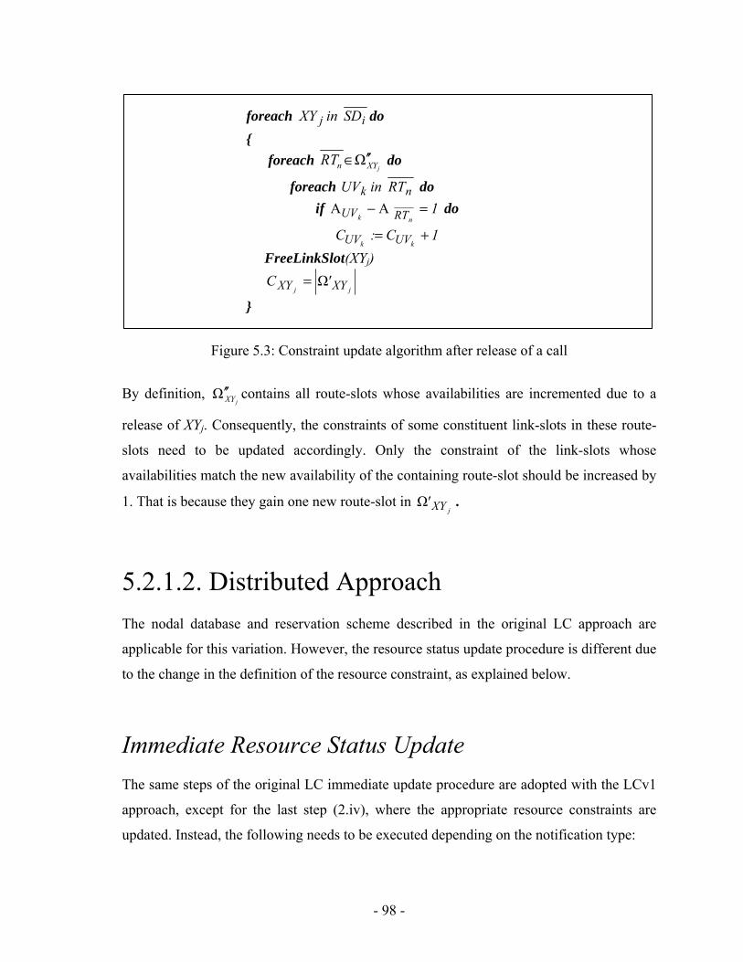
- 98 -
Figure 5.3: Constraint update algorithm after release of a call
By definition, jXYΩ ′′ contains all route-slots whose availabilities are incremented due to a
release of XYj. Consequently, the constraints of some constituent link-slots in these route-
slots need to be updated accordingly. Only the constraint of the link-slots whose
availabilities match the new availability of the containing route-slot should be increased by
1. That is because they gain one new route-slot in jXY'Ω .
5.2.1.2. Distributed Approach
The nodal database and reservation scheme described in the original LC approach are
applicable for this variation. However, the resource status update procedure is different due
to the change in the definition of the resource constraint, as explained below.
Immediate Resource Status Update
The same steps of the original LC immediate update procedure are adopted with the LCv1
approach, except for the last step (2.iv), where the appropriate resource constraints are
updated. Instead, the following needs to be executed depending on the notification type:
foreach ij SDinXY do foreach
jXYnRT Ω ′′∈ do
foreach nk RTinUV do
if 1nk RTUV =− ΑΑ do
1C:Ckk UVUV +=
FreeLinkSlot(XYj)
jj XYXY 'C Ω=

- 99 -
a. Reservation Notification: Indentify the route-slot availability kSDΑ which would be
the minimum availability in the LSAL of the corresponding CRSL entry. First, if
kSDΑ is equal to iXYΑ and also equal to
jUVΑ , deduct 1 from the constraint of the
corresponding local link-slot UVj. Second, deduct 1 from the availability of XYi in the
CRSL LSAL. Note that the source node that sends the notification should update the
availability of XYi, and its constraint by counting the number of intersecting route-
slots that matches its new availability.
b. Release Notification: Indentify the route-slot availability kSDΑ which would be the
minimum availability in the LSAL of the corresponding CRSL entry. If kSDΑ is
equal to iXYΑ , check the CRSL LSAL for other link-slots that has the same
availability. First, if no link-slots other than XYi are identified and ji UVXY 1 Α=+Α ,
then add 1 to the constraint of the corresponding local link-slot UVj. Second, add 1 to
the availability of XYi in the CRSL LSAL. Note that the source node that sends the
notification should update the availability of XYi, and its constraint by counting the
number of intersecting route-slots that matches its new availability.
Periodic Resource Status Update
The same steps of the original LC periodic update procedure are adopted with the LCv1
approach, except for the last step (3.ii), where the appropriate resource constraints are
updated. Instead, the following step needs to be processed for every link-slot that is
included in the received notification:
- Set the corresponding link-slot availability in the CRSL LSAL to the availability of the
considered link-slot XYi. Identify the new route-slot availability kSDΑ which would be
the minimum availability in the LSAL of the corresponding CRSL entry. Calculate the
constraint of the corresponding local link-slot UVj by counting the number of
intersecting route-slots that have the same availability.
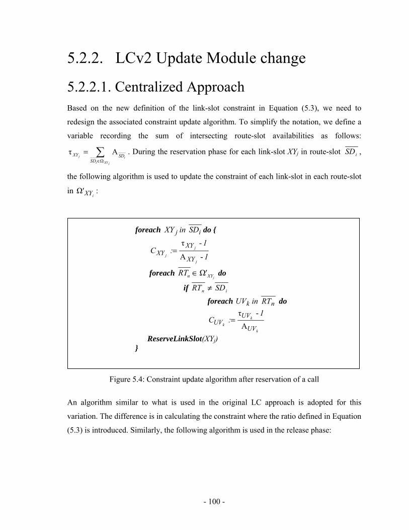
- 100 -
5.2.2. LCv2 Update Module change
5.2.2.1. Centralized Approach
Based on the new definition of the link-slot constraint in Equation (5.3), we need to
redesign the associated constraint update algorithm. To simplify the notation, we define a
variable recording the sum of intersecting route-slot availabilities as follows:
∈
=jXYi
ij
SDSDXY
Ω
Ατ . During the reservation phase for each link-slot XYj in route-slot iSD ,
the following algorithm is used to update the constraint of each link-slot in each route-slot
in iXY'Ω :
Figure 5.4: Constraint update algorithm after reservation of a call
An algorithm similar to what is used in the original LC approach is adopted for this
variation. The difference is in calculating the constraint where the ratio defined in Equation
(5.3) is introduced. Similarly, the following algorithm is used in the release phase:
foreach ij SDinXY do
1
1:C
j
j
jXY
XYXY -Α
-τ=
foreach jXYn 'RT Ω∈ do
if in SDRT ≠
foreach nk RTinUV do
k
k
kUV
UVUV
1:C
Α
-τ=
ReserveLinkSlot(XYj)

- 101 -
Figure 5.5: Constraint update algorithm
5.2.2.2. Distributed Approach
The same concepts described in the original distributed LC approach are applicable with
variation 2. The only difference is in the method used at each node in calculating the
constraints of its local link-slots according to Equation (5.3). The constraint here is equal
to the recorded number of available intersecting route-slots divided by the link-slot
availability. Note that the link-slot availability here is always up to date since it is a local
variable that does not depend on external parameters. However, the recorded number of
available intersecting route-slots would most likely be outdated since it depends on
external parameters that get reconciled at every update.
5.3. Simulation Results In this section, we compare the performance of the LC approach variations in single and
multi-fibre environments. Our observations are based on simulations using the simulation
parameters described in Chapter 3. We focus on the multi-fibre case since all the described
variations become identical when calculating the constraint of a resource in a single-fibre
foreach ij SDinXY do
1
1:C
j
j
jXY
XYXY +
+=Α
τ
foreach jXYnRT Ω ′′∈ do
if in SDRT ≠
foreach nk RTinUV do
k
k
kUV
UVUV
1:C
Α
τ +=
FreeLinkSlot(XYj)

- 102 -
network. In a single fibre network,
∈
=′∈∀==jXYi
ijjij
SDSDXYXYiSDXY 'SD11
Ω
ΑΩΩΑΑ . Thus, the behavior of
LCv1 approach is identical to the original LC approach in a single fiber environment.
Similarly,
∈
∈==
jXYi
i
j
jXYi
i
j
SDSD
XY
SDSD
XY 1Ω
ΩΑ
Α
Α
Α confirming that the behavior of LCv2
approach and the original LC approach are identical in a single fiber environment. Thus,
the performance of original LC, LCv1, and LCv2 approaches should converge in single
fiber networks. Figure (5.6) showing the performance of all LC approach variations in a
single-fibre environment confirms this observation.
1.E-06
1.E-05
1.E-04
1.E-03
1.E-02
1.E-01
1.E+00
30 35 40 45 50 80 120
Load (Erlang)
Blo
ckin
g pr
obab
ility
LCv1 LC FF LCv2
Figure 5.6: Performance of all LC approach variations in a single-fibre environment

- 103 -
Figure (5.7) compares the performance of the LC approach variations in a multi-fiber
network. It shows that the different variations of the LC approach produced a slightly
better performance which is closer to the optimum level than the original LC approach.
Note that the optimum performance level is achieved by the First Fit approach with OTSI.
1.E-06
1.E-05
1.E-04
1.E-03
1.E-02
1.E-01
1.E+00
100 150 200 250 300 350 400
Load (Erlang)
Blo
ckin
g pr
obab
ility
LCv1 LC FF LCv2 FF+OTSI
Figure 5.7: Performance of the LC approach variations in a multi-fiber network
Figure (5.8) compares the performance of the distributed LC approach with different
variations in a multi-fiber network where no status update is applied after a brief initial
period (not included in the chart). It shows that the variation of the LCv2 approach
produces the closest performance to the optimal case of the FF approach with OTSI. The
resulting performance is slightly better than what is achieved with the original LC
approach. The LCv1 approach produces the worst performance which is close to the worst
case scenario of the FF approach without OTSI. The results are slightly better at low loads

- 104 -
and converge to the results of the FF approach without OTSI at medium and high loads.
Figure (5.9) shows the same performance trend when the status update rate is 1 per 103
calls.
The difference in performance stems from the resource constraint definitions of the LCv1
approaches. In a multi-fiber network, a link-slot constraint based on the LCv1 approach
tends to be significantly less than its constraint based on the original LC approach. In
principle, ∈
≤jXYi
ij
SDSDXY'
Ω
ΑΩ since jj XYXY' ΩΩ ⊆ . However, the inequality is more
likely than the equality. Equality is possible only when jj XYXY' Ω=Ω and
ji XYiSD SD1 ΩΑ ∈∀= which is a rare case in a multi fibers system. Thus, the constraint
is a route-slots counter with a range between 0 and r, where r is the average number of
routes intersecting on a given link; it reflects the number of route-slots whose availabilities
are reduced when the link-slot is reserved. It does not reflect the total number of available
route-slots that could use the link-slot as defined in the original LC approach. Therefore,
the resulting order from the outdated ωt (defined in Chapter 4) is not based on the status of
all route-slots in the network. It is rather a partial order based on route-slot counters rather
than the availabilities of all route-slots. The resulting priorities of the route-slots in all
routes according to the constraints collected by the last update are not accurately
synchronized. Back to the traffic lights system analogy, an order organizing traffic based
on a very limited view of the map cannot reduce traffic jams.

- 105 -
1.E-06
1.E-05
1.E-04
1.E-03
1.E-02
1.E-01
1.E+00
100 150 200 250 300 350 400
Load (Erlang)
Blo
ckin
g pr
obab
ility
LCv1 LC FF LCv2 FF+OTSI
Figure 5.8: Performance of the distributed LC approach with different variations in a multi-
fiber network (with no updates)

- 106 -
1.E-06
1.E-05
1.E-04
1.E-03
1.E-02
1.E-01
1.E+00
100 150 200 250 300 350 400
Load (Erlang)
Blo
ckin
g pr
obab
ility
LCv1 LC FF LCv2 FF+OTSI
Figure 5.9: Performance of the distributed LC approach with different variations in a multi-fiber network (with update rate of 1 per 103 calls)
5.4. Conclusion In this chapter, we identified two variations of the original LC approach, LC Approach
based on Route-Slot Count (LCv1), and LC Approach based on Availability Ratio (LCv2).
Both variations slightly enhance network performance in the multi-fiber case reaching the
optimum performance level of the FF approach with OTSI. However, the performance of
all considered LC approaches converge in the single-fiber case as it is expected. The LCv2
approach produced the best results in the case of periodic or no status updates as compared
to the LCv1 and the original LC approaches. On the other hand, the performance of the
LCv1 approach exceeded the worst performance level of the FF approach in the cases of

- 107 -
periodic or no status updates. As a conclusion, the LCv2 approach outperformed the LCv1
and the original LC approaches and should be adopted as the standard LC approach.

- 108 -
6. Optimized Passive Optical Time-Slot Interchanger
6.1. Introduction A major concern with the POTSI architecture that we proposed in [Maach2004] is its bulky
size and the insertion loss caused by the coupling of optical signals at each delay unit.
Although a POTSI has the smallest size in terms of fiber length as compared to other OTSI
architectures which we described in the background chapter, it is still considered bulky. It
takes about 2 km of fiber lines to delay a traffic segment by 10 µs. If an OTDM frame of
64 time slots (10 µs each) is adopted, we need 128 km of fiber lines to build a POTSI. In
addition, the passive signal flow inside a POTSI comes at the cost of insertion loss. As the
signal propagates from one FDL to another, it loses some of its power at the joint point. To
mitigate the insertion loss factor, we need to interleave a few amplifiers among the FDLs
depending on the loss ratio of employed optical couplers and fiber lines inside the POTSI.
The more and longer the FDLs used inside a POTSI, the more amplifiers are required to
restore the fading signal, which increases the overall equipment cost. Based on these
limitations, we propose in this chapter a new optimized form of POTSI, the Limited Range
POTSI (POTSI-LR). We reduce the number of FDLs to a fraction of the number of time
slots in the frame (N), which will consequently reduces the POTSI’s bulkiness, the
crossbar size and the number of required amplifiers. It was proven in the literature that a
limited range wavelength converter, having a 30 percent conversion range, achieves the
same network performance as a full-range converter [Zeineddine1998]. Similarly, we
believe that the same conclusion, if not better, can be applied in the case of POTSI-LR. In
addition, we propose the sharing of POTSIs amongst the output links of a switch as
opposed to using dedicated POTSI per link. We also propose and investigate the effect of

- 109 -
interleaving POTSIs among network nodes as opposed to deploying a POTSI in each node.
Before discussing the simulation results, we briefly define the use of the POTSI
architecture as an efficient tool for time slot synchronization between two adjacent nodes.
Finally, due to the apparent functional similarity between OTSI and optical wavelength
converter, we dedicate a section summarizing the similarity and differences between the
two devices.
6.2. Limited-Range POTSI (POTSI-LR) A POTSI as defined in [Maach2004] has N FDLs, equal to the number of time slots in a
TDM frame, and is said to be of size N. We define the POTSI-LR to be a POTSI of size M,
where NM < . A POTSI-LR has an interchanging-range of N
M and is capable of delaying
a time slot i to a time slot j if NMiji <+<< , or ( ) NmodMij0 +<< , where i and j
are slot positions in a TDM frame of size N. Table (6.1) compares the characteristic of
POTSI-LR versus regular POTSI. It clearly shows the reduction in fibre length and
crossbar size achieved by POTSI-LR. Figure (6.1) describes the high level architecture of a
POTSI-LR. It is quite similar to the POTSI in Figure (2.7), but with less FDLs.
Delay Lines per
OTSI Crossbar
Size Fiber
Length Switching operations
POTSI 1 × N-1 N 1
POTSI-LR size M (1 < M < N)
1 × M M 1
Table 6.1: OTSI Architecture Comparison
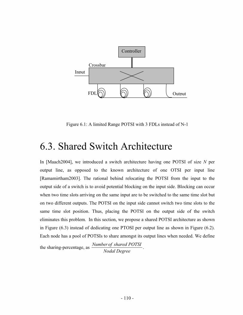
- 110 -
Figure 6.1: A limited Range POTSI with 3 FDLs instead of N-1
6.3. Shared Switch Architecture In [Maach2004], we introduced a switch architecture having one POTSI of size N per
output line, as opposed to the known architecture of one OTSI per input line
[Ramamirtham2003]. The rational behind relocating the POTSI from the input to the
output side of a switch is to avoid potential blocking on the input side. Blocking can occur
when two time slots arriving on the same input are to be switched to the same time slot but
on two different outputs. The POTSI on the input side cannot switch two time slots to the
same time slot position. Thus, placing the POTSI on the output side of the switch
eliminates this problem. In this section, we propose a shared POTSI architecture as shown
in Figure (6.3) instead of dedicating one PTOSI per output line as shown in Figure (6.2).
Each node has a pool of POTSIs to share amongst its output lines when needed. We define
the sharing-percentage, as DegreeNodal
POTSIsharedofNumber.
Controller
Crossbar
FDL
Input
Output

- 111 -
Figure 6.2: Dedicated POTSI Architecture of a 4 x 4 switch
Figure 6.3: Shared OTSI Architecture of a 4 x 4 switch having 2 POTSIs
Controller
Input Output
CrossbarPOTSI
Controller
Input Output
Crossbar
POTSI

- 112 -
6.4. OTSI Vs Wavelength Converter By definition, an all-optical wavelength converter (OWC) converts wavelength λx to λy by
pure optical means without opto-electronic processing. Similarly, OTSI converts between
time slots instead of wavelengths. At this point, many researchers concluded that both
devices would yield similar results in terms of network performance. In fact, this
conclusion is not very precise. An OWC can serve only one call, riding on a wavelength,
during a given period; on the other hand, an OTSI can serve multiple concurrent calls,
riding on different time slots during the same period. Thus, it is closer to the truth to say
that an OTSI, in an OTDM node, achieves similar performance improvement to a bank of
N OWCs in a Wavelength Routed Optical Network (WRON) node, where N is the number
of time slots per frame in the network.
We say that the above conclusion is very close to the truth, and not completely true,
because of a little discrepancy when considering limited-range conversion. A full range
converter covers the whole spectrum of wavelengths in a WDM system. A limited range
converter covers a subset of the WDM spectrum; the covered spectrum is relative to the
input wavelength, and is between –k and +k from that wavelength. A wavelength within a
distance j from the boundaries of the WDM spectrum, where j < k, cannot take full
conversion advantage of the limited range converter. In contrast, thinking of a limited
range OTSI, we see that this limitation does not exist. An interchanger has the capability of
delaying one time slot beyond its frame boundaries to another time slot in the next frame.
One final discrepancy is the size. Wavelength converters are tiny in size as compared to the
bulky nature of the OTSI. As defined, an OTSI is made of a number of FDLs each having a
delay capacity equal to one time slot. By a quick calculation, we derive that 2 km of fiber
is needed to form one FDL that delays a time slot equal to 10 μs. Given that the diameter
of a single mode fiber is around 150 μm, the volume of one FDL cable is close to 45 cm3.

- 113 -
6.5. POTSI Based Synchronizers In the background chapter, we reviewed the usage of delay lines as synchronizers that
realign incoming frames to the local switch’s time slot boundaries [Bononi1999,
Liew2003]. We also learned that the internal architecture of a synchronizer resembles the
architecture of an OTSI. In this section, we propose a POTSI-based synchronizer hoping to
introduce a more feasible solution to the synchronization problem. The POTSI-based
synchronizer is made of k FDLs, each having a delay duration g. The duration g is equal to
the guard time separating each pair of adjacent time slots in the TDM frame. The number
of FDLs k is equal to the slot time µ divided by g (i.e. g
μ), assuming that g>μ . The time
slot can be considered as a series of k mini-time-slots of size g, labelled from 0 to k-1. If
the propagation delay and the clock difference between two adjacent switches are equal to
d and c respectively, the time slot shift with respect to the receiving switch is
( ) ( )gmodcd ++ μ . In this case, the signal has to be adjusted in the synchronizer by
passing through ( ) ( )
g
gmodcd ++ μ FDLS. Note that the remainder of this division is less
than g, and hence is covered by the guard time. To know the time slot shift between two
adjacent nodes, a predetermined probe signal equal to one time slot must be sent
occasionally from the upstream to the downstream node. The downstream node should
keep sensing for the signal at every time slot. Upon receipt, the downstream node measures
the un-received portion of the signal which would basically be the time slot shift with the
upstream node. The signalling operation between adjacent nodes can be performed over a
dedicated wavelength, or over any idle one for an efficient bandwidth usage. Figure (6.4) is
a schematic representation of a POTSI-based synchronizer and the essential parameters.
As an elaborative example, if the guard time is 2 and the time slot is 10, the synchronizer
should have 5 FDLs of size 2. If the propagation delay and clock difference between two
nodes are 47 and 4 respectively, the signal has to be adjusted by hopping through
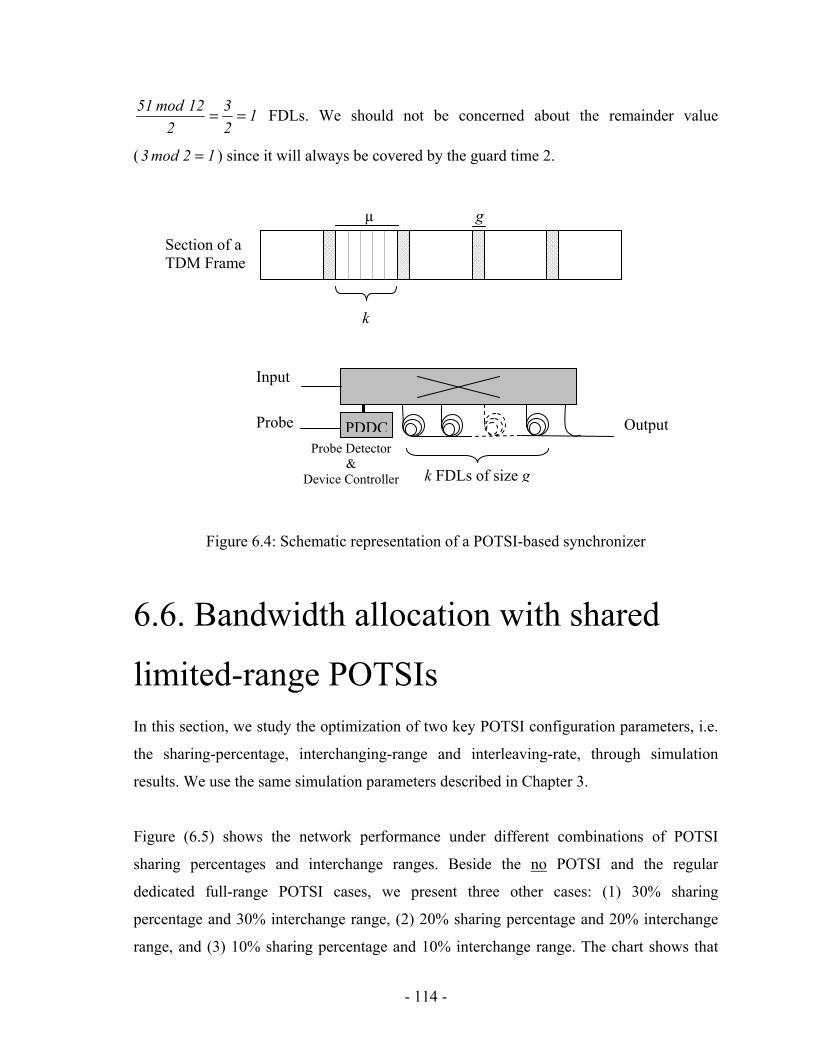
- 114 -
12
3
2
12mod51 == FDLs. We should not be concerned about the remainder value
( 12mod3 = ) since it will always be covered by the guard time 2.
Figure 6.4: Schematic representation of a POTSI-based synchronizer
6.6. Bandwidth allocation with shared
limited-range POTSIs In this section, we study the optimization of two key POTSI configuration parameters, i.e.
the sharing-percentage, interchanging-range and interleaving-rate, through simulation
results. We use the same simulation parameters described in Chapter 3.
Figure (6.5) shows the network performance under different combinations of POTSI
sharing percentages and interchange ranges. Beside the no POTSI and the regular
dedicated full-range POTSI cases, we present three other cases: (1) 30% sharing
percentage and 30% interchange range, (2) 20% sharing percentage and 20% interchange
range, and (3) 10% sharing percentage and 10% interchange range. The chart shows that
k
g µ
PDDC
k FDLs of size g
Probe Detector &
Device Controller
Input
Output Probe
Section of a TDM Frame
- 115 -
30% sharing percentage and 30 percentage interchange range should be enough to yield the
same performance gain resulting from the dedicated full POTSI case.
1.E-06
1.E-05
1.E-04
1.E-03
1.E-02
1.E-01
30 35 40 45 50
Load (Erlang)
Blo
ckin
g P
rob
abil
ity
S=0%-R=0% S=100%-R=100% S=30%-R=60%
S=30%-R=30% S=30%-R=10%
Figure 6.5: The effects of varying the POTSI’s sharing-percentages (S%) and interchanging ranges (R%) in NSF network
Since the charts in Figure (6.5) are generated based on the NSFNET topology where the
average nodal degree is close to 3, we do not have data for cases where the POTSI’s
sharing is below 30%. To bypass this limitation, we employ a star topology of 20 edge
nodes with a POTSI-equipped core. The results of varying the POTSI sharing percentage
in the core node are plotted in Figure (6.6). The charts show that when the interchange
range is at 30% or above, varying the sharing percentage has no substantial impact on
performance. However, performance degrades slightly when the sharing percentage is
10%. On the other hand, if the interchange range is below 30%, any reduction on the
sharing percentage clearly degrades network performance. The worst case scenario is
noticed when both the sharing percentage and interchange range are at 10%. On the other

- 116 -
hand, when both parameters are 30%, the network produced a performance close to the
optimum case of dedicated full-range POTSIs.
4.E-03
5.E-03
6.E-03
7.E-03
8.E-03
9.E-03
100 50 30 20 10
Interchange Range (%)
Blo
ckin
g P
rob
abil
ity
S=100% S=50% S=30% S=20% S=10% S=0%
Figure 6.6: The effects of varying POTSI’s sharing-percentage (S%) and interchanging
range in a star network of 20 edge nodes, with load 60 Erlang
The charts in Figure (6.7) and (6.8) are generated based on a 14 nodes ring topology. They
are meant to study the effect of interleaving POTSIs among nodes instead of using these
devices at each node. Some nodes are equipped with POTSI and others have none. The
interleaving rate reflects the number of POTSI-equipped nodes with respects to the total
number of nodes. In addition, the distribution of POTSI-equipped nodes is uniform; i.e., if
the interleaving rate is 1/x, we know that there should be a PTOSI-equipped node every x
nodes on the ring. For both charts, the number of POTSIs inside the POTSI-equipped
nodes is 1, or 50% of the nodal degree in a bidirectional ring. It is not possible to go lower

- 117 -
than 50%; and, going higher is proven to yield the same performance. Figure (6.7) shows
that as the POTSI’s interleaving rate gets smaller, the network performance degrades
substantially. An interleaving rate of 0.5, one POTSI at every second node, produces a
performance very close to the dedicated full-range POTSI. The most interesting result
shown on the chart is when the interleaving rate is 0.75, i.e. one non-POTSI-equipped node
every 4 nodes.
1.E-05
1.E-04
1.E-03
1.E-02
1.E-01
1.E+00
15 20 25 30 35 40
Load (Erlang)
Blo
ck
ing
Pro
ba
bili
ty
I=1 I=0.5 I=0.33 I=0.25
I=0.2 No POTSI I=0.75
Figure 6. 7: Blocking probability in a 14-Nodes Ring topology, when interleaving POTSIs
amongst nodes at different rate (I)
Figure (6.8) shows the effect of varying the OTSI interleaving rate on a 14-nodes ring
network loaded at 35 Erlang. The chart shows that when the rate is less than 0.5, the
network performance degrades at a steeper rate. On the other hand, performance

- 118 -
degradation is less steep when the rate is above 0.5. An interleave rate of 0.5 seems to offer
an acceptable performance level with a decent saving in the number of deployed POTSIs.
1.E-03
1.E-02
1.E-01
0 0.2 0.25 0.33 0.5 0.66 0.75 0.8 0.9 1
POTSI Interleaving Rate
Blo
ckin
g P
rob
abil
ity
Figure 6.8: Blocking probability in a 14-Nodes Ring topology, when varying the POTSIs Interleaving Rate between 0 and 1, at a fixed load of 35 Erlang
Figure (6.9) shows the effect of varying the interchanging range in the case where the
interleaving rate is 0.5. When the interchanging range is 30% or 50%, the network
performance remains close to the case where the range is 100%. Lowering the
interchanging range to 10% degrades performance drastically. Thus, based on the
information reported in charts (6.7), (6.8) and (6.9), we say that interleaving POTSIs in a
ring network at a 0.5 rate, where each POTSI-equipped node has a POTSI sharing
percentage and interchange range of 50%, respectively, yields a performance improvement
close to the optimum level which is reported for the dedicated full-range POTSI case.

- 119 -
1.E-05
1.E-04
1.E-03
1.E-02
1.E-01
1.E+00
15 20 25 30 35 40
Load (Erlang)
Blo
ckin
g P
rob
abil
ity
I=1-R=100% I=0.5-R=100% I=0.5-R=50%
I=0.5-R=30% I=0.5-R=10% No POTSI
Figure 6.9: Blocking probability in a 14-node ring topology, with POTSI’s interleaving rate (I) 0.5, and various percentages of interchanging ranges (R%)
6.7. Conclusion Compared to the family of optical time slot interchangers noted in the literature, the
passive optical time slot interchanger (POTSI), proposed in an earlier work [Maach2004],
has the best number of switching operations, crossbar size and total fibre length. In this
chapter, we proposed an optimized form of POTSI, Limited-Range POTSI (POTSI-LR),
whose capability is limited to switching a time slot to a subset of nearby time slots in the
frame instead of all possible time slots. In addition, we investigated the sharing and
interleaving of POTSI-LR as opposed to dedicating one POTSI to each ongoing link.
Relying on simulation results, we showed that deploying shared limited-range POTSIs can
achieve blocking probabilities very close to those of dedicated full-range POTSIs. In fact,
the POTSI sharing-percentage can be as small as 20% of the nodal degree together with an
interchanging-range as small as 30%. Thus, the overall cost and crossbar complexity can

- 120 -
be substantially reduced while still maintaining close to optimal performance gains. In
addition, we showed that POTSIs can be interleaved at a 0.5 rate and still produces a close
to optimum performance, even with a sharing percentage and interchange rate of 50%.
Finally, we discussed in this chapter the use of POTSIs to build efficient time slot
synchronizers between adjacent nodes.

- 121 -
7. Conclusions
7.1. Summary In Optical TDM (OTDM) networks, transmission between two adjacent nodes must be
synchronized to ensure proper data processing and avoid loss. Synchronization in an
OTDM network is the process of ensuring that each OTDM switch receives a time sliced
traffic segment right at the start of a time slot based on its local clock. If the same time slot
(in a TDM frame) must be maintained throughout a communication channel between a
source-destination pair, frame boundary synchronization is required among all network
nodes. On the other hand, slot boundary synchronization should be adequate if maintaining
the same slot location over a communication channel is not essential. Several papers in the
literature assumed frame boundary synchronization, and hence treated a time slot as a
small communication channel that is continuous from source to destination. This
assumption helped the authors to employ wavelength allocation schemes to solve the slot
reservation problem since a communication channel, based on the same time slot across a
route, can be seen as a subdivision of a wavelength. On the other hand, if assuming slot
boundary synchronization, the wavelength allocation schemes cannot solve the slot
reservation question since the time slot continuity is not maintained for a communication
channel. Slot reservation schemes that reserve a series of time slot across a given route are
required in this case. Some papers considered the First Fit (FF), Random Fit (RF) and
Least Loaded (LL) schemes to handle slot reservation in OTDM networks synchronized on
slot boundary. None of these schemes, under fixed routing algorithms, comes close to
optimum in terms of network performance. The optimum OTDM network performance,
under fixed routing algorithms, can be identified by assuming unlimited optical
interchanging capacity at each node which allows the interchange from any slot to any
other slot. In our thesis, we used the FF scheme with full optical time slot interchangers
(OTSI) as an optimal benchmark against which we measured our results. Aiming to avoid
- 122 -
optical buffering or slot interchanging and still maintain close to optimal performance, we
proposed the Least Constraining (LC) Slot Allocation scheme as a novel bandwidth
reservation method for all-optical TDM networks without buffering. The link-slot
constraint is measured by the sum of availabilities of the route-slots on the intersecting
routes that can use the link-slot at a given point in time. In addition, the route-slot
constraint is equal to the sum of all constituent link-slot constraints. The LC schemes
allocate the least constraining route-slot. After several simulation runs based on uniform
and non-uniform traffic, backed by an analytical discussion based on uniform traffic only,
we proved that the LC schemes provide close to optimum performance in OTDM networks
without buffering. The results are consistent under uniform and non-uniform traffic, mesh
and ring topology, single and multi-fiber, and fixed and alternate fixed routing.
Aiming to apply the LC approach in GMPLS networks, we designed a distributed LC
scheme. We defined the essential nodal database and basic parameters that should be added
to the RSVP-TE or CR-LDP signaling messages used in GMPLS networks. In the
proposed distributed scheme, resource status update may be immediate or periodic.
Immediate updates are broadcasted for each reserved or released resource immediately
after the reservation or release operation. On the other hand, periodic updates are
exchanged among all nodes in the network at a fixed time interval, reporting status changes
in their managed resources since the last status update. The periodic update approach is
essential to incorporate the LC resource status update into GMPLS, which relies on global
periodic updates using OSPF or IS-IS link state update mechanisms. In this case, the LC
approach must maintain its proven performance gain under this limitation. We proved that
an update rate greater than or equal to α
1 maintains close to optimal performance, where α
is the probability that the least-constraining route-slot on a route changes after an accepted
call arrival. Reducing the update rate to any value below α
1, the network performance
degrades to a fixed level but still better than the worst performance of the FF approach.
Thus, after an initial period of immediate updates, we can stop all subsequent updates and
still get a performance level as good as obtained by update rates lower than α
1. On the

- 123 -
other hand, when varying the status update rate in multi-fiber environments, the
performance remains stable at the improved level achieved by the immediate update
approach. In this case, it is possible to stop resource updates after a brief period of
immediate updates and still achieve close to optimal performance. That would substantially
save the signaling bandwidth for status updates and the associated processing power, in
addition to facilitating the deployment in a GMPLS network.
Interested in investigating the performance of the LC scheme when varying the definition
of a resource constraint, we proposed two variations. As a first variation of the LC scheme,
we modified the definition of a link-slot constraint to be the number of intersecting route-
slots that might use the slot at a given point in time, instead of the sum of availabilities of
these route-slots. As a second variation, we changed the link-slot constraint definition to be
the sum of intersecting route-slots availabilities divided by the link-slot availability. Both
variations slightly enhanced network performance in the multi-fiber case, reaching the
optimum performance level of the FF approach with OTSI. However, the performance of
all LC variations converged in the single-fiber. The second variation produced the best
results in the case of periodic or no status updates as compared to the first variation and the
original LC approaches. On the other hand, the performance of the first variation exceeded
the worst performance level of the FF approach in the cases of periodic or no status
updates. As a conclusion, the second variation outperformed the other variations and
should be adopted as the standard LC approach.
Although the LC scheme eliminates the need for Optical Time-Slot Interchangers (OTSI)
to improve network performance, we proposed in this thesis an enhancement to the Passive
OTSI (POTSI), which was introduced in a separate joint work with Dr. Abdul Maach.
Compared to the family of optical time slot interchangers noted in the literature, a POTSI
has the best number of switching operations, crossbar size and total fibre length. The
enhanced version of POTSI is limited to switching a time slot to a subset of nearby time
slots in the frame instead of all possible time slots. We called it Limited-Range POTSI
(POTSI-LR). To further optimize the usage of POTSIs in a network, we investigated the
sharing and interleaving of POTSI-LR as opposed to dedicating one POTSI to each

- 124 -
ongoing link. The sharing of limited-range POTSIs achieved a network performance close
to the case of dedicated full-interchanging-range POTSIs. We proved that a sharing-
percentage equal to 20% of the nodal degree and an interchanging-range equal to 30% of
the frame size maintained essentially the same performance achieved by dedicated full-
interchanging-range POTSIs. This approach reduces the overall cost and crossbar
complexity. In addition, we showed that POTSIs can be interleaved at a 0.5 rate and still
produces a close to optimum performance, even with a sharing percentage and interchange
rate of 50% respectively. Although, OTSIs are not needed with the LC scheme, we still
need optical buffering to build synchronizers at the end of each fiber link in order to adjust
the propagation delay of the link to a multiple of the slot time. Therefore, we proposed the
use of the POTSI architecture as an efficient solution to construct synchronizers between
adjacent nodes.
7.2. Overview of Contributions Over the course of developing our thesis, we made the following contributions:
• The Least Constraining (LC) slot allocation scheme: We proposed the LC slot
allocation scheme as the main contribution in this thesis. It is designed to provide close
to optimal performance in all-optical TDM networks, synchronized on slot boundaries
and with no buffering. The optimal performance is measured by the employment of
full-range dedicated OTSIs along with the FF allocation scheme. The LC scheme
proved its superiority over other optical time-slot allocation schemes in single or multi-
fiber environments, fixed or alternative routing schemes, uniform or non-uniform
traffic, and mesh or ring topologies [Zeineddine2007].
• A distributed approach to the LC scheme in GMPLS network: We proposed a
distributed approach to the LC scheme in an attempt to make it deployable in a GMPLS
network. Beside defining the nodal database and essential messaging, the main
challenge was to reduce the associated link-state signalling overhead. In addition,
GMPLS relies on periodic link-state updates. We proved that the distributed LC
scheme in a multi-fiber environment does not require any update after an initial period

- 125 -
of immediate updates to maintain close to optimal performance. On the other hand, if
stopping the updates in a single-fiber environment, performance degrades to a fixed
level but does not converge to the worst performance level reported with the FF
approach [Zeineddine2009].
• Variations of the LC scheme: We proposed two variations of the original LC scheme
aiming to improve performance to a level closer to optimum. The variations are based
on modifying the definition of the resource constraint. Both variations showed slight
performance improvement over the original LC scheme in a multi-fiber environment
and converged to the same performance level in the single fiber case.
• Limited-Range Passive Optical Time-Slot Interchanger (POTSI-LR): We proposed
an enhancement to the Passive OTSI architecture by reducing the number of the
constituent fiber delay lines to a fraction of N, where N is the number of time-slots in a
TDM frame. The main goal was to reduce the device size and overall cost and still
maintain the same performance achieved by a full range POTSI, which has N fiber
delay lines. We showed that an interchange range equal to 30% of N achieves
practically the same performance gain as a full interchange range [Zeineddine2006].
• Shared OTSI: We proposed a shared OTSI architecture for an optical TDM switch
instead of a dedicated OTSI per output line. The aim is to reduce the number of
utilized OTSIs per node and still maintain the same performance achieved by the
dedicated OTSI architecture. We showed that an OTSI sharing percentage equal to 20
% of the nodal degree is enough to maintain practically the same performance gain as
the dedicated OTSI approach [Zeineddine2006].
• Interleaved OTSI: We proposed the interleaving of OTSIs among network nodes
instead of equipping every node with these devices. The aim is to reduce the number of
utilized OTSIs in the global network and still maintain the performance achieved by the
regular OTSI approach. We showed that an OTSI interleaving rate of 0.5 yields a
performance level close to what is achieved with the case of having OTSIs at every
node.
• Using POTSI as synchronizers: We proposed the usage of POTSI as an effective
solution to the synchronization problem along the link between two adjacent nodes.

- 126 -
Over the years of graduate studies and work toward this thesis, we participated in the
following projects:
• A bandwidth allocation scheme in Optical TDM network: Dr. Abdul Maach and I
proposed a new scheme to share network resources using Time Division Multiplexing
(TDM) instead of the statistical multiplexing employed in optical burst switching. To
avoid contention and improve bandwidth utilization, we defined a simple reservation
scheme that guarantees time slot deliveries as far as the bandwidth is available. In
addition, we proposed the POTSI architecture as a simplified form of OTSI. The
POTSI was used to solve the contention problem, and improve performance. The
proposed scheme can simultaneously serve many classes of traffic by adjusting some
bandwidth allocation parameters [Maach2004].
• Deploying AAPN in legacy networks: Dr. Sofia Parades and I proposed deployment
approaches for the Agile All-Photonic Network (AAPN) project over legacy networks.
The legacy systems are assumed to be made of IP routers connected to a network of
Reconfigurable Add-Drop Multiplexers (ROADM) and Wavelength Selective Switches
(WSS). In our solutions, we proposed the partitioning of the mesh network into
intersected rings, each forming an autonomous domain. ROADMs are used to bridge
traffic between two intersected rings. Another solution was to use static wavelength
allocation to exclusively assign at least one wavelength to each node. The wavelengths
assigned to a node are the only communication channels through which it receives
traffic from other nodes. The project was under the AAPN umbrella and partially
funded by JDSU.
7.3. Future Work For further expansions of the work described in our thesis, we list the following topics of
future work:
• Investigate solutions to employ the LC scheme along with dynamic routing protocols
instead of fixed routing. We proved the efficiency of the LC scheme with fixed and

- 127 -
alternative routing schemes; however, we did not consider dynamic routing since the
definition of link-slot constraints is based on the assumption of predetermined routes.
• Study the scalability problem of the distributed LC scheme in terms of nodal database
size and messaging volume; investigate solutions to reduce the amount of saved and
exchanged information. In the thesis, we focused on the signalling problem and paid
little attention to the scalability concerns related to the size of the managed and
exchanged information.
• Study the technological and economical constraints for the realization of POTSI-LR.
Although we proposed the POTSI and POTSI-LR architecture, we did not investigate
the technological limits of a feasible POTSI. A PTOSI is made of series of individual
fiber delay lines and a switch fabric, patched together via passive couplers. Therefore, a
signal passing through a POTSI would loose a fair amount of its signal as it passes
from one fiber delay line to another. Some of the important questions are: how can
signal amplification help in this case? - And, how many amplifiers do we need and
where should they be deployed?

- 128 -
References
[Banerjee2001] A. Banerjee et al, “Generalized Multiprotocol Label Switching: An
Overview of Routing and Management Enhancements,” IEEE Commun. Mag., vol. 39, no.
1, Jan. 2001.
[Blumenthal1994] D. Blumenthal, P. Prucnal, and J. Sauer, “Photonic packet switches:
architectures and experimental implementations,” Proc. IEEE, Vol. 82, pp. 1650–1667,
November 1994.
[Bochmann2004] G. Bochmann, T. Hall, O. Yang, M. Coates, L. Mason, and R. Vickers,
“The Agile All Photonic Network: An Architectural Outile,” Queen’s Biennial Conference
on Communications, February 2004.
[Bononi1999] A. Bononi, Optical Networking (Ref to Synchornizer), Published by
Springer, 1999.
[Chen2004] A. Chen, A. Wong, and C. Lea, “Routing and Time-Slot Assignment in
Optical TDM Networks,” IEEE Journal on Selected Areas in Communications, Vol. 22,
No. 9, November 2004.
[Colle2003] D. Colle, J. Cheyns, C. Develder, E. Van Breusegem, A. Ackaert, M.
Pickavet, and P. Demeester, “GMPLS extensions for supporting advanced optical
networking technologies,” 5th International Conference on Transparent Optical Networks,
Vol. 1, pp. 170 – 173, June 2003.
[Hafid2005a] A. Hafid and A. Maach, “A Novel Resources Provisioning Scheme in Time
Slotted Optical Networks,” IEEE International Conference on Communications, 2005, Vol.
3, pp. 1641-1645, May 2005.

- 129 -
[Hafid2005b] A. Hafid, A. Maach, J. Drissi, “DARISON: A Distributed Advance
Reservation System for Interconnected Optical Networks,” Conference on Optical
Network Design and Modeling, pp. 85-92, February 2005.
[Helsinki2004] J. Helsinki, “OSPF and IS-IS Evolution,” The Pennsylvania State
University CiteSeer Archives, 2004.
[Huang2000] N. Huang, G. Liaw, and C. Wang, “A Novel All-Optical Transport Network
with Time-Shared Wavelength Channels,” IEEE Journal on Selected Areas in
Communications, Vol. 18, No. 10, October 2000.
[Lang2004] J. P. Lang, Y. Rekter, and D. Papadimitriou, “RSVP-TE Extensions in Support
of End-to-End Generalized Multiprotocol Label Switching (GMPLS)-Based Recovery,”
Internet draft, draft-ietf-ccamp-gmpls-recovery-e2e-signaling-02.txt, 2004.
[Liew2003] S. Liew and H. Chao, “On Slotted WDM Switching in Buffereless All-Optical
Networks,” Proc. IEEE High Performance Interconnects '03, 11th Symposium, pp. 96 -101,
August 2003.
[Liu2005a] X. Liu, A. VinoKurov, and L. Mason, “Performance Comparison of OTDM
and OBS Scheduling for Agile All-Photonic Network,” Proc. IFIP Metropolitan Area
Network Conference, Ho Chi Minh City, Vietnam, April 2005.
[Liu2005b] X. Liu, N. Saberi, M. Coates and L. Mason, “A Comparison between Time-slot
Scheduling Approaches for All-Photonic Networks,” Proc. IEEE ICICS, Bangkok ,
Thailand , December 2005.
[Maach2004] A. Maach, H. Zeineddine and G. Bochmann, “A bandwidth Allocation
Scheme in Optical TDM Network,” Proc. IEEE International Conference on High Speed

- 130 -
Networks and Multimedia Communications (HSNMC), Toulouse, Springer LNCS, pp.
801-812, July 2004.
[Mei1997] Y. Mei and C. Qiao, “Efficient Distributed Control Protocols for WDM All-
Optical Networks,” Proc. 6th International Conference on Computer Communications and
Networks, p. 150, 1997.
[Nuzman2006] C. Nuzman and I. Widjaja, “Time-domain Wavelength Interleaved
Networking with Wavelength Reuse,” Proc. IEEE INFOCOM 2006.
[Pattayina2000] A. Pattavina, M. Martinelli, and G. Maier, “Techniques and Technologies
towards All-Optical Switching,” Optical Networking Magazine, pp.75-93, Apr. 2000.
[Peng2006] C. Peng, G. Bochmann and T. Hall, “Quick Birkhoff-von Neumann
Decomposition Algorithm for Agile All-Photonic Network Cores,” IEEE International
Conference on Communications, Istanbul Turkey, Vol. 6, pp. 2593-2598, June 2006.
[Qiao1997] C. Qiao and R. Melhem, “Reducing Communication Latency with Path
Multiplexing in Optically Interconnected Multiprocessor Systems,” IEEE Transactions on
Parallel and Distributed Systems, Vol. 8, pp. 97-108, February 1997.
[Qiao1999] C. Qiao and M. Yoo, “Optical burst switching (OBS)–a new paradigm for an
optical Internet,” Journal of High Speed Networks, Vol. 8, no. 1, pp. 69–84, 1999.
[Ramakrishna2005] Bo Wen, Ramakrishna, and Krishna Sivalingam, “Routing,
Wavelength and Time-Slot-Assignment Algorithm for Wavelength-Routed Optical
WDM/TDM Networks,” Journal of Lightwave Technology, vol. 23, No. 9, September
2005.
[Ramamirtham2003] J. Ramamirtham and J. Turner, “Time Sliced Optical Burst
Switching,” Proc. IEEE INFOCOM 2003, San Francisco, California, April 2003.

- 131 -
[Ramaswami2002] R. Ramaswami, K.N., Sivarajan, “Optical Networks, A Practical
Perspective,” 2nd ed. Published by Morgan Kaufmann Publishers, 2002.
[RFC1629] R. Colella et al, Guidelines for OSI NSAP Allocation in the Internet, May
1994.
[RFC2205] E. Braden et al, Resource Reservation Protocol (RSVP), September 1997.
[RFC2328] J. Moy, OSPF Version 2, April 1998.
[RFC3031] E. Rosen et al, Multiprotocol Label Switching Architecture, January 2001.
[RFC3036] L. Anderson et al, LDP Specification, October 2001. (obsoleted by RFC5036,
October 2007).
[RFC3209] D. Awduche et al, RSVP-TE: Extensions to RSVP for LSP Tunnels, December
2001.
[RFC3212] B. Jamoussi et al, Constraint-Based LSP Setup using LDP. Network Working
Group, January 2002.
[RFC3471] P. Ashwood-Smith et al, “Generalized MPLS — Signaling Functional
Description,” April 2001.
[RFC3472] P. Ashwood-Smith et al, “Generalized MPLS Signaling—CR-LDP
Extensions,” Internet draft, draft-ietf-mplsgeneralized-cr-ldp-02.txt, Apr. 2001, work in
progress.
[RFC3630] D. Katz et al, Traffic Engineering (TE) Extensions to OSPF Version 2,
September 2003.
- 132 -
[RFC3945] E Mannie, Generalized Multi-Protocol Label Switching (GMPLS)
Architecture, October 2004.
[RFC4136] P. Pillay-Esnault, OSPF Refresh and Flooding Reduction in Stable Topologies,
July 2005.
[RFC4203] K. Kompella et al, “OSPF Extensions in Support of Generalized MPLS,”
March 2001.
[RFC4205] K. Kompella et al, “IS-IS Extensions in Support of Generalized MPLS,” March
2001.
[RFC4974] P. Ashwood-Smith et al, “Generalized MPLS Signaling — RSVP-TE
Extensions,” April 2001.
[Saberi2004] N. Saberi, and M. Coates “Bandwidth Reservation in Optical WDM/TDM
Star Networks,” Queens Biennial Symposium on Communications, Kingston, Canada,
June 2004.
[Shaikh2001] A. Shaikh, J. Rexford, and K. G. Shin, “Evaluating the impact of stale link
state on quality-of-service routing,” IEEE/ACM Transactions on Networking, Vol. 9, pp.
162–176, April 2001.
[Shen2004] S. Shen, G. Xiao, and T. H. Cheng, “Evaluating the impact of the link-state
update period on the blocking performance of wavelength-routed networks,” Proc. Optical
Fiber Communication Conference (OFC), February 2004.
[Shen2006] S. Shen, G. Xiao, and T. Cheng, “The Performance of Periodic Link-State
Update in Wavelength-Routed Networks,” 3rd International Conference on Broadband
Communications, Networks and Systems, San Jose, CA, pp. 1-10, October 2006.

- 133 -
[Siew2006] C. Siew, D. Xue, Y. Qin, and J. Schmitt “Providing Deterministic Quality of
Service in Slotted Optical Networks,” Optics Express, Vol. 14, Issue 26, pp. 12679-12692,
December 2006.
[Srinivasan2002] R. Srinivasan, A. Somani, “A Generalized Framework for Analyzing
Time-Space Switched Optical Networks,” IEEE Journal on Selected Areas in
Communications, Vol. 20, No. 1, January 2002.
[Subramaniam2000] S. Subramaniam, J. Harder, and H. Choi, “Scheduling Multirate
Sessions in Time Division Multiplexed Wavelength-Routing Networks,” IEEE Journal on
Selected Areas in Communications, Vol. 18, No. 10, October 2000.
[Sukhni2008] E. Sukhni, and Hussein T. Mouftah: Parallel Fixed-Alternative-Routing
Based Provisioning Framework for Distributed Controlled Survivable WDM Mesh
Networks. 6th Annual Communication Networks and Services Research Conference
(CNSR), Halifax, Canada, pp. 287-294, May 2008.
[Turner1999] J. Turner, “Terabit Burst Switching,” Journal of High Speed Networks, Vol.
8, pp 3-16, March 1999.
[Vinokurov2005] A. Vinokurov, X. Liu, and L. Mason, “Resource sharing for QoS in
Agile All Photonic Networks”, OPNETWORK 2005, Washington D.C., August 2005.
[Vokkarane2003] V. Vokkarane and J. Jue, “Segmentation-based non-preemptive
scheduling algorithms for optical burstswitched networks,” Proc. First International
Workshop on Optical Burst Switching (WOBS), October 2003.
[Wang2006] Z. Wang, N. Chi, and S. Yu, “Time-Slot Assignment Using Optical Buffer
With a Large Variable Delay Range Based on AVC Crosspoint Switch,” J. Lightwave
Technol. 24, 2994- (2006).

- 134 -
[Widjaja2004] I. Widjaja and I. Saniee, “Simplified Layering and Flexible Bandwidth with
TWIN,” Proc. SIGCOMM FDNA Workshop, Portland August 2004
[Yang2007a] W. Yang, S. Paredes, T. Hall, “A Study of the Impact of Stale Information on
the Blocking Performance of Dynamic Routing, Wavelength and Timeslot Assignment
Scheme for Bandwidth on Demand in Metro Agile All-Optical Networks,” Photonics
North 2007, Ottawa, Canada, June 2007.
[Yang2007b] W. Yang, S. Paredes, T. Hall, “A Study of Fast Flexible Bandwidth
Assignment Methods and their Blocking Probabilities for Metro Agile All-optical Ring
Networks,” IEEE International Conference on Communications (ICC-2007), Glasgow,
Scotland, 24-28 June 2007.
[Yao2000] S. Yao, B. Mukherjee, S. Yoo, and S. Dixit, "All-Optical Packet-Switched
Networks: A Study of Contention Resolution Schemes in an Irregular Mesh Network with
Variable-Sized Packets," Proceedings of SPIE OptiComm 2000.
[Yates1999] J. M. Yates, J. Lacey, and D. Everitt, “Blocking in multiwavelength TDM
networks,” Telecommunication Systems Journal, vol. 12, no. 1, pp. 1-19, August 1999.
[Yuan1996] X. Yuan, R. Gupta, and R. Melhem, “Distributed Control in Optical WDM
Networks,” IEEE Conf. on Military Communications, McLean, VA , October 1996.
[Yuan1997] X. Yuan, R. Gupta, and R. Melhem, “Distributed Path Reservation Algorithms
for Multiplexed All-Optical Interconnection Networks,” International Symposium on High
Performance Computer Architecture - HPCA-3, 1997.
[Zang1999] H. Zang, J. Jue, and B. Mukherjee, “Photonic Slot Routing in All-Optical
WDM Mesh Networks,” Proc. IEEE Globecom '99, Rio de Janeiro, Brazil, December
1999.

- 135 -
[Zang2000] H. Zang, J. Jue, and B. Mukherjee, “Capacity Allocation and Contention
Resolution in a Photonic Slot Routing All-optical WDM Mesh Network,” Journal of
Lightwave Technology, Vol. 18, No. 12, December 2000.
[Zeineddine1998] H. Zeineddine, A. Jakel, S. Bandyopadhayay, A. Sengupta “Efficacy of
Wavelength Translation in all-Optical Networks,” Proc. International Conference on
Computing and Information (ICCI), pp. 43-50, June 1998.
[Zeineddine2006] H. Zeineddine, P. He, and G. Bochmann, “Optimization Analysis of
Optical Time Slot Interchanges in All-Optical Network,” Proc. IASTED Wireless and
Optical Communications, Banf Alberta, pp. 207-212, July 2006.
[Zeineddine2007] H. Zeineddine and G. Bochmann, “Least Constrained Slot Allocation in
Optical TDM Networks,” Proc. asdxczIEEE International Conference on Wireless and
Optical Communications Networks, Singapore, pp. 1 – 5, July 2007.
[Zeineddine2009] H. Zeineddine and G. Bochmann, “A Distributed Algorithm for the
Least Constraining Slot Allocation in MPLS Optical Networks,” IEEE International
Conference on Communications, Dresden, Germany, June 2009.