least squares adjustment: linear and nonlinear weighted regression...

Least Squares Adjustment:Linear and Nonlinear Weighted Regression Analysis

Allan Aasbjerg Nielsen

Technical University of DenmarkNational Space Institute/Informatics and Mathematical Modelling

Building 321, DK-2800 Kgs. Lyngby, Denmarkphone +45 4525 3425, fax +45 4588 1397

e-mail [email protected]/∼aa

29 August 2012

Preface

This note primarily describes the mathematics of least squares regression analysis as it is often used ingeodesy including land surveying and satellite based positioning applications. In these fields regression isoften termed adjustment1. The note also contains a couple of typical land surveying and satellite positioningapplication examples. In these application areas we are typically interested in the parameters of the model(often 2- or 3-D positions) and their uncertainties and not in predictive modelling which is often the mainconcern in other regression analysis applications.

Adjustment is often used to obtain estimates of relevant parameters in an over-determined system of equationswhich may arise from deliberately carrying out more measurements than actually needed to determine the setof desired parameters. An example may be the determination of a geographical position based on informationfrom a number of Global Navigation Satellite System (GNSS) satellites also known as space vehicles (SV).It takes at least four SVs to determine the position (and the clock error) of a GNSS receiver. Often more thanfour SVs are used and we use adjustment to obtain a better estimate of the geographical position (and theclock error) and to obtain estimates of the uncertainty with which the position is determined.

Regression analysis is used in many other fields of application both in the natural, the technical and the socialsciences. Examples may be curve fitting, calibration, establishing relationships between different variablesin an experiment or in a survey, etc. Regression analysis is probably one the most used statistical techniquesaround.

Dr. Anna B. O. Jensen provided insight and data for the Global Positioning System (GPS) example.

Matlab code and sections that are considered as either traditional land surveying material or as advancedmaterial are typeset with smaller fonts.

Comments in general or on for example unavoidable typos, shortcomings and errors are most welcome.

1in Danish “udjævning”

2 Least Squares Adjustment

Contents

Preface 1

Contents 2

1 Linear Least Squares 4

1.1 Ordinary Least Squares, OLS . . . . . . . . . . . . . . . . . . . . . . . . . . . . . . . . . . 7

1.1.1 Linear Constraints . . . . . . . . . . . . . . . . . . . . . . . . . . . . . . . . . . . 8

1.1.2 Parameter Estimates . . . . . . . . . . . . . . . . . . . . . . . . . . . . . . . . . . 8

1.1.3 Dispersion and Significance of Estimates . . . . . . . . . . . . . . . . . . . . . . . 11

1.1.4 Residual and Influence Analysis . . . . . . . . . . . . . . . . . . . . . . . . . . . . 13

1.1.5 Singular Value Decomposition, SVD . . . . . . . . . . . . . . . . . . . . . . . . . 15

1.1.6 QR Decomposition . . . . . . . . . . . . . . . . . . . . . . . . . . . . . . . . . . . 15

1.1.7 Cholesky Decomposition . . . . . . . . . . . . . . . . . . . . . . . . . . . . . . . . 15

1.2 Weighted Least Squares, WLS . . . . . . . . . . . . . . . . . . . . . . . . . . . . . . . . . 16


1.2.2 Weight Assignment . . . . . . . . . . . . . . . . . . . . . . . . . . . . . . . . . . . 18


1.2.4 WLS as OLS . . . . . . . . . . . . . . . . . . . . . . . . . . . . . . . . . . . . . . 24

1.3 General Least Squares, GLS . . . . . . . . . . . . . . . . . . . . . . . . . . . . . . . . . . 24

2 Nonlinear Least Squares 24

2.1 Nonlinear WLS by Linearization . . . . . . . . . . . . . . . . . . . . . . . . . . . . . . . . 26


2.1.2 Iterative Solution . . . . . . . . . . . . . . . . . . . . . . . . . . . . . . . . . . . . 27


2.1.4 Confidence Ellipsoids . . . . . . . . . . . . . . . . . . . . . . . . . . . . . . . . . 28

2.1.5 Dispersion of a Function of Estimated Parameters . . . . . . . . . . . . . . . . . . . 29

2.1.6 The Derivative Matrix . . . . . . . . . . . . . . . . . . . . . . . . . . . . . . . . . 29

2.2 Nonlinear WLS by other Methods . . . . . . . . . . . . . . . . . . . . . . . . . . . . . . . 46

Allan Aasbjerg Nielsen 3

2.2.1 The Gradient or Steepest Descent Method . . . . . . . . . . . . . . . . . . . . . . . 46

2.2.2 Newton’s Method . . . . . . . . . . . . . . . . . . . . . . . . . . . . . . . . . . . . 47

2.2.3 The Gauss-Newton Method . . . . . . . . . . . . . . . . . . . . . . . . . . . . . . 47

2.2.4 The Levenberg-Marquardt Method . . . . . . . . . . . . . . . . . . . . . . . . . . . 49

3 Final Comments 49

Literature 50

Index 52


1 Linear Least Squares

Example 1 (from Conradsen, 1984, 1B p. 5.58) Figure 1 shows a plot of clock error as a function of timepassed since a calibration of the clock. The relationship between time passed and the clock error seems tobe linear (or affine) and it would be interesting to estimate a straight line through the points in the plot, i.e.,estimate the slope of the line and the intercept with the axis time = 0. This is a typical regression analysistask (see also Example 2). [end of example]

0 5 10 15 20 25 30 35 40 45 500

0.5

1

1.5

2

2.5

3

3.5

4

4.5

Time [days]

Clo

ck e

rror

[sec

onds

]

Figure 1: Example with clock error as a function of time.

Let’s start by studying a situation where we want to predict one (response) variable y (as clock error inExample 1) as a linear function of one (predictor) variable x (as time in Example 1). When we have onepredictor variable only we talk about simple regression. We have n joint observations of x (x1, . . . , xn) andy (y1, . . . , yn) and we write the model where the parameter θ1 is the slope of the line as

y1 = θ1x1 + e1 (1)y2 = θ1x2 + e2 (2)

... (3)yn = θ1xn + en. (4)

The eis are termed the residuals; they are the differences between the data yi and the model θ1xi. Rewrite toget

e1 = y1 − θ1x1 (5)e2 = y2 − θ1x2 (6)

... (7)en = yn − θ1xn. (8)

In order to find the best line through (the origo and) the point cloud {xi yi}ni=1 by means of the least squares


principle write

ϵ =1

2

n∑i=1

e2i =1

2

n∑i=1

(yi − θ1xi)2 (9)

and find the derivative of ϵ with respect to the slope θ1

dϵ

dθ1=

n∑i=1

(yi − θ1xi)(−xi) =n∑

i=1

(θ1x2i − xiyi). (10)

Setting the derivative equal to zero and denoting the solution θ1 we get

θ1n∑

i=1

x2i =

n∑i=1

xiyi (11)

or (omitting the summation indices for clarity)

θ1 =

∑xiyi∑x2i

. (12)

Since

d2ϵ

dθ21=

n∑i=1

x2i > 0 (13)

for non-trivial cases θ1 gives a minimum for ϵ. This θ1 gives the best straight line through the origo and thepoint cloud, “best” in the sense that it minimizes (half) the sum of the squared residuals measured along they-axis, i.e., perpendicular to the x-axis. In other words: the xis are considered as uncertainty- or error-freeconstants, all the uncertainty or error is associated with the yis.

Let’s look at another situation where we want to predict one (response) variable y as an affine function of one(predictor) variable x. We have n joint observations of x and y and write the model where the parameter θ0is the intercept of the line with the y-axis and the parameter θ1 is the slope of the line as

y1 = θ0 + θ1x1 + e1 (14)y2 = θ0 + θ1x2 + e2 (15)

... (16)yn = θ0 + θ1xn + en. (17)

Rewrite to get

e1 = y1 − (θ0 + θ1x1) (18)e2 = y2 − (θ0 + θ1x2) (19)

... (20)en = yn − (θ0 + θ1xn). (21)

In order to find the best line through the point cloud {xi yi}ni=1 (and this time not necessarily through theorigo) by means of the least squares principle write

ϵ =1

2

n∑i=1

e2i =1

2

n∑i=1

(yi − (θ0 + θ1xi))2 (22)


and find the partial derivatives of ϵ with respect to the intercept θ0 and the slope θ1

∂ϵ

∂θ0=

n∑i=1

(yi − (θ0 + θ1xi))(−1) = −n∑

i=1

yi + nθ0 + θ1n∑

i=1

xi (23)

∂ϵ

∂θ1=

n∑i=1

(yi − (θ0 + θ1xi))(−xi) = −n∑

i=1

xiyi + θ0n∑

i=1

xi + θ1n∑

i=1

x2i . (24)

Setting the partial derivatives equal to zero and denoting the solutions θ0 and θ1 we get (omitting the summa-tion indices for clarity)

θ0 =

∑x2i

∑yi −

∑xi

∑xiyi

n∑

x2i − (

∑xi)2

(25)

θ1 =n∑

xiyi −∑

xi∑

yin∑

x2i − (

∑xi)2

. (26)

We see that θ1∑

xi + nθ0 =∑

yi or y = θ0 + θ1x (leading to∑

ei =∑[yi − (θ0 + θ1xi)] = 0) where

x =∑

xi/n is the mean value of x and y =∑

yi/n is the mean value of y. Another way of writing this is

θ0 = y − θ1x (27)

θ1 =

∑(xi − x)(yi − y)∑

(xi − x)2=

σxy

σ2x

. (28)

where σxy =∑(xi − x)(yi − y)/(n− 1) is the covariance between x and y, and σ2

x =∑(xi − x)2/(n− 1) is

the variance of x. Also in this case θ0 and θ1 give a minimum for ϵ, see page 8.

Example 2 (continuing Example 1) With time points (xi) [3 6 7 9 11 12 14 16 18 19 23 24 33 35 39 41 42 4445 49]T days and clock errors (yi) [0.435 0.706 0.729 0.975 1.063 1.228 1.342 1.491 1.671 1.696 2.122 2.1812.938 3.135 3.419 3.724 3.705 3.820 3.945 4.320]T seconds we get θ0 = 0.1689 seconds and θ1 = 0.08422seconds/day. This line is plotted in Figure 1. Judged visually the line seems to model the data fairly well.

[end of example]

More generally let us consider n observations of one dependent (or response) variable y and p′ independent(or explanatory or predictor) variables xj, j = 1, . . . , p′. The xjs are also called the regressors. Whenwe have more than one regressor we talk about multiple regression analysis. The words “dependent” and“independent” are not used in their probabilistic meaning here but are merely meant to indicate that xj inprinciple may vary freely and that y varies depending on xj . Our task is to 1) estimate the parameters θj inthe model below, and 2) predict the expectation value of y where we consider y as a function of the θjs andnot of the xjs which are considered as constants. For the ith set of observations we have

yi = yi(θ0, θ1, . . . , θp′ ;x1, . . . , xp′) + ei (29)= yi(θ;x) + ei (30)= yi(θ) + ei (31)= (θ0 + ) θ1xi1 + · · ·+ θp′xip′ + ei, i = 1, . . . , n (32)

where θ = [θ0 θ1 . . . θp′ ]T , x = [x1 . . . xp′ ]

T , and ei is the difference between the data and the model forobservation i with expectation value E{ei} = 0. ei is termed the residual or the error. The last equation aboveis written with the constant or the intercept θ0 in parenthesis since we may want to include θ0 in the model orwe may not want to, see also Examples 3-5. Write all n equations in matrix form

y1y2...yn

=

1 x11 · · · x1p′

1 x21 · · · x2p′

...... . . . ...

1 xn1 · · · xnp′

θ0θ1...θp′

+

e1e2...en

(33)


or

y = Xθ + e (34)

where

• y is n× 1,

• X is n× p, p = p′ + 1 if an intercept θ0 is estimated, p = p′ if not,

• θ is p× 1, and

• e is n× 1 with expectation E{e} = 0.

If we don’t want to include θ0 in the model, θ0 is omitted from θ and so is the first column of ones in X .

Equations 33 and 34 are termed the observation equations2. The columns in X must be linearly independent,i.e., X is full column rank. Here we study the situation where the system of equations is over-determined,i.e., we have more observations than parameters, n > p. f = n − p is termed the number of degrees offreedom3.

The model is linear in the parameters θ but not necessarily linear in y and xj (for instance y could be replacedby ln y or 1/y, or xj could be replaced by √

xj , extra columns with products xkxl called interactions could beadded to X or similarly). Transformations of y have implications for the nature of the residual.

Finding an optimal θ given a set of observed data (the ys and the xjs) and an objective function (or a cost ora merit function, see below) is referred to as regression analysis in statistics. The elements of the vector θ arealso called the regression coefficients. In some application sciences such as geodesy including land surveyingregression analysis is termed adjustment4.

All uncertainty (or error) is associated with y, the xjs are considered as constants which may be reasonableor not depending on (the genesis of) the data to be analyzed.

1.1 Ordinary Least Squares, OLS

In OLS we assume that the variance-covariance matrix also known as the dispersion matrix of y is propor-tional to the identity matrix, D{y} = D{e} = σ2I , i.e., all residuals have the same variance and they areuncorrelated. We minimize the objective function ϵ = 1/2

∑ni=1 e

2i = eTe/2 (hence the name least squares:

we minimize (half) the sum of squared differences between the data and the model, i.e., (half) the sum of thesquared residuals)

ϵ = 1/2(y −Xθ)T (y −Xθ) (35)= 1/2(yTy − yTXθ − θTXTy + θTXTXθ) (36)= 1/2(yTy − 2θTXTy + θTXTXθ). (37)

The derivative with respect to θ is

∂ϵ

∂θ= −XTy +XTXθ. (38)

2in Danish “observationsligningerne”3in Danish “antal frihedsgrader” or “antal overbestemmelser”4in Danish “udjævning”


When the columns of X are linearly independent the second order derivative ∂2ϵ/∂θ∂θT = XTX is positivedefinite. Therefore we have a minimum for ϵ. Note that the p× p XTX is symmetric, (XTX)T = XTX .

We find the OLS estimate for θ termed θOLS (pronounced theta-hat) by setting ∂ϵ/∂θ = 0 to obtain thenormal equations5

XTXθOLS = XTy. (39)

1.1.1 Linear Constraints

Linear constraints can be build into the normal equations by defining

KTθ = c (40)

where the vector c and the columns of matrix K define the constraints, one constraint per column of K and per element of c. If forexample θ = [θ1 θ2 θ3 θ4 θ5]

T and θ2, θ3 and θ5 are the three angles in a triangle which must sum to 200 gon (with no constraintson θ1 and θ4), use KT = [0 1 1 0 1] and c = 200 gon.

Also, we must add a term to the expression for ϵ in Equation 35 above setting the constraints to zero

L = ϵ+ λT (KTθ − c) (41)

where λ is a vector of so-called Lagrangian multipliers.

Setting the partial derivatives of Equations 41 and 40 to zero leads to[XTX K

KT 0

] [θOLS

λ

]=

[XTyc

]. (42)

1.1.2 Parameter Estimates

If the symmetric matrix XTX is “well behaved”, i.e., it is full rank (equal to p) corresponding to linearlyindependent columns in X a formal solution is

θOLS = (XTX)−1XT y. (43)

For reasons of numerical stability especially in situations with nearly linear dependencies between the columnsof X (causing slight alterations to the observed values in X to lead to substantial changes in the estimated θ;this problem is known as multicollinearity) the system of normal equations should not be solved by invertingXTX but rather by means of SVD, QR or Cholesky decomposition, see Sections 1.1.5, 1.1.6 and 1.1.7.

If we apply Equation 43 to the simple regression problem in Equations 14-17 of course we get the samesolution as in Equations 25 and 26 (as an exercise you may want to check this).

When we apply regression analysis in other application areas we are often interested in predicting the responsevariable based on new data not used in the estimation of the parameters or the regression coefficients θ. Inland surveying and GNSS applications we are typically interested in θ and not on this predictive modelling.

(In the linear case θOLS can be found in one go because eTe is quadratic in θ; unlike in the nonlinear casedealt with in Section 2 we don’t need an initial value for θ and an iterative procedure.)

5in Danish “normalligningerne”


�

��

��

�

�

Figure 2: y is the projection of y onto the hyperplane spanned by the vectors xi in the columns of matrix X(modified from Hastie, Tibshirani and Friedman (2009) by Jacob S. Vestergaard).

The estimate for y termed y (pronounced y-hat) is

y = XθOLS = X(XTX)−1XTy = Hy (44)

where H = X(XTX)−1XT is the so-called hat matrix since it transforms or projects y into y (H “putsthe hat on y”). In geodesy (and land surveying) these equations are termed the fundamental equations6. His a projection matrix: it is symmetric, H = HT , and idempotent, HH = H . We also have HX = X andthat the trace of H , trH = tr(X(XTX)−1XT ) = tr(XTX(XTX)−1) = trIp = p.

The estimate of the error term e (also known as the residual) termed e (pronounced e-hat) is

e = y − y = y −Hy = (I −H)y. (45)

Also I −H is symmetric, I −H = (I −H)T , and idempotent, (I −H)(I −H) = I −H . We also have(I −H)X = 0 and tr(I −H) = n− p.

X and e, and y and e are orthogonal: XT e = 0 and yT e = 0. Geometrically this means that our analysisfinds the orthogonal projection y of y onto the hyperplane spanned by the linearly independent columns ofX . this gives the shortest distance between y and y, see Figure 2.

Since the expectation of θOLS

E{θOLS} = E{(XTX)−1XTy} (46)= (XTX)−1XTE{y} (47)= (XTX)−1XTE{Xθ + e} (48)= θ, (49)

θOLS is unbiased or a central estimator.

Example 3 (from Strang and Borre, 1997, p. 306) Between four points A, B, C and D situated on a straightline we have measured all pairwise distances AB, BC, CD, AC, AD and BD. The six measurements arey = [3.17 1.12 2.25 4.31 6.51 3.36]T m. We wish to determine the distances θ1 = AB, θ2 = BC andθ3 = CD by means of linear least squares adjustment. We have n = 6, p = 3 and f = 3. The six observation

6in Danish “fundamentalligningerne”


equations are

y1 = θ1 + e1 (50)y2 = θ2 + e2 (51)y3 = θ3 + e3 (52)y4 = θ1 + θ2 + e4 (53)y5 = θ1 + θ2 + θ3 + e5 (54)y6 = θ2 + θ3 + e6. (55)

In matrix form we get (this is y = Xθ + e; units are m)

3.171.122.254.316.513.36

=

1 0 00 1 00 0 11 1 01 1 10 1 1

θ1θ2θ3

+

e1e2e3e4e5e6

. (56)

The normal equations are (this is XTXθ = XTy; units are m) 3 2 12 4 21 2 3

θ1θ2θ3

=

13.9915.3012.12

. (57)

The hat matrix is

H =

1/2 −1/4 0 1/4 1/4 −1/4−1/4 1/2 −1/4 1/4 0 1/4

0 −1/4 1/2 −1/4 1/4 1/41/4 1/4 −1/4 1/2 1/4 01/4 0 1/4 1/4 1/2 1/4

−1/4 1/4 1/4 0 1/4 1/2

. (58)

The solution is θ = [3.1700 1.1225 2.2350]T m, see Matlab code in page 12.

Now, let us estimate an intercept θ0 also corresponding to an imprecise zero mark of the distance measuringdevice used. In this case we have n = 6, p = 4 and f = 2 and we get (in m)

3.171.122.254.316.513.36

=

1 1 0 01 0 1 01 0 0 11 1 1 01 1 1 11 0 1 1

θ0θ1θ2θ3

+

e1e2e3e4e5e6

. (59)

The normal equations in this case are (in m)6 3 4 33 3 2 14 2 4 23 1 2 3

θ0θ1θ2θ3

=

20.7213.9915.3012.12

. (60)


The hat matrix is

H =

3/4 0 1/4 1/4 0 −1/40 3/4 0 1/4 −1/4 1/4

1/4 0 3/4 −1/4 0 1/41/4 1/4 −1/4 1/2 1/4 00 −1/4 0 1/4 3/4 1/4

−1/4 1/4 1/4 0 1/4 1/2

. (61)

The solution is θ = [0.0150 3.1625 1.1150 2.2275]T m, see Matlab code in page 12. [end of example]

1.1.3 Dispersion and Significance of Estimates

Dispersion or variance-covariance matrices for y, θOLS , y and e are

D{y} = σ2I (62)D{θOLS} = D{(XTX)−1XTy} (63)

= (XTX)−1XTD{y}X(XTX)−1 (64)= σ2(XTX)−1 (65)

D{y} = D{XθOLS} (66)= XD{θOLS}XT (67)= σ2H , V{yi} = σ2Hii (68)

D{e} = D{(I −H)y} (69)= (I −H)D{y}(I −H)T (70)= σ2(I −H) = D{y} − D{y}, V{ei} = σ2(1−Hii). (71)

The ith diagonal element of H , Hii, is called the leverage7 for observation i. We see that a high leveragegives a high variance for yi indicating that observation i is poorly predicted by the regression model. Thisagain indicates that observation i may be an outlier, see also Section 1.1.4 on residual and influence analysis.

For the sum of squared errors (SSE, also called RSS for the residual sum of squares) we get

eT e = yT (I −H)y (72)

with expectation E{eT e} = σ2(n− p). The mean squared error MSE is

σ2 = eT e/(n− p) (73)

and the root mean squared error RMSE is σ also known as s. σ = s has the same unit as ei and yi.

The square roots of the diagonal elements of the dispersion matrices in Equations 62, 65, 68 and 71 are thestandard errors of the quantities in question. For example, the standard error of θi denoted σθi is the squareroot of the ith diagonal element of σ2(XTX)−1.

Example 4 (continuing Example 3) The estimated residuals in the case with no intercept are e = [0.0000

−0.0025 0.0150 0.0175 −0.0175 0.0025]T m. Therefore the RMSE or σ = s =√eT e/3 m = 0.0168 m.

7in Danish “potentialet”


The inverse of XTX is 3 2 12 4 21 2 3

−1

=

1/2 −1/4 0−1/4 1/2 −1/4

0 −1/4 1/2

. (74)

This gives standard deviations for θ, σθ = [0.0119 0.0119 0.0119]T m. The case with an intercept givesσ = s = 0.0177 m and standard deviations for θ, σθ = [0.0177 0.0153 0.0153 0.0153]T m. [end of example]

So far we have assumed only that E{e} = 0 and that D{e} = σ2I , i.e., we have made no assumptions about the distribution of e.Let us further assume that the eis are independent and identically distributed (written as iid) following a normal distribution. ThenθOLS (which in this case corresponds to a maximum likelihood estimate) follows a multivariate normal distribution with mean θand dispersion σ2(XTX)−1. Assuming that θi = ci where ci is a constant it can be shown that the ratio

zi =θi − ciσθi

(75)

follows a t distribution with n− p degrees of freedom. This can be used to test whether θi − ci is significantly different from 0. Iffor example zi with ci = 0 has a small absolute value then θi is not significantly different from 0 and xi should be removed fromthe model.

Example 5 (continuing Example 4) The t-test statistics zi with ci = 0 in the case with no intercept are [266.3 94.31 187.8]T

which are all very large compared to 95% or 99% percentiles in a two-sided t-test with three degrees of freedom, 3.182 and 5.841respectively. The probabilities of finding larger values of |zi| are [0.0000 0.0000 0.0000]T . Hence all parameter estimates aresignificantly different from zero. The t-test statistics zi with ci = 0 in the case with an intercept are [0.8485 206.6 72.83 145.5]T ;all but the first value are very large compared to 95% and 99% percentiles in a two-sided t-test with two degrees of freedom,4.303 and 9.925 respectively. The probabilities of finding larger values of |zi| are [0.4855 0.0000 0.0002 0.0000]T . Therefore theestimate of θ0 is insignificant (i.e., it is not significantly different from zero) and the intercept corresponding to an imprecise zeromark of the distance measuring device used should not be included in the model. [end of example]

Often a measure of variance reduction termed the coefficient of determination denoted R2 and a version thatadjusts for the number of parameters denoted R2

adj are defined in the statistical literature:

SST0 = yTy (if no intercept θ0 is estimated)SST1 = (y − y)T (y − y) (if an intercept θ0 is estimated)SSE = eT eR2 = 1− SSE/SSTi

R2adj = 1− (1−R2)(n− i)/(n− p) where i is 0 or 1 as indicated by SSTi.

Both R2 and R2adj lie in the interval [0,1]. For a good model with a good fit to the data both R2 and R2

adj

should be close to 1.Matlab code for Examples 3 to 5

% (C) Copyright 2003% Allan Aasbjerg Nielsen% [email protected], www.imm.dtu.dk/˜aa

% model without intercept

y = [3.17 1.12 2.25 4.31 6.51 3.36]’;X = [1 0 0; 0 1 0; 0 0 1; 1 1 0; 1 1 1; 0 1 1];[n,p] = size(X);f = n-p;

thetah = X\y;yh = X*thetah;eh = y-yh;s2 = eh’*eh/f;s = sqrt(s2);iXX = inv(X’*X);Dthetah = s2.*iXX;stdthetah = sqrt(diag(Dthetah));


t = thetah./stdthetah;pt = betainc(f./(f+t.ˆ2),0.5*f,0.5);

H = X*iXX*X’;Hii = diag(H);

% model with intercept

X = [ones(n,1) X];[n,p] = size(X);f = n-p;

thetah = X\y;yh = X*thetah;eh = y-yh;s2 = eh’*eh/f;s = sqrt(s2);iXX = inv(X’*X);Dthetah = s2.*iXX;stdthetah = sqrt(diag(Dthetah));t = thetah./stdthetah;pt = betainc(f./(f+t.ˆ2),0.5*f,0.5);

H = X*iXX*X’;Hii = diag(H);

The Matlab backslash operator “\” or mldivide, “left matrix divide”, in this case with X non-square computes the QR factor-ization (see Section 1.1.6) of X and finds the least squares solution by back-substitution.

Probabilities in the t distribution are calculated by means of the incomplete beta function evaluated in Matlab by the betaincfunction.

1.1.4 Residual and Influence Analysis

Residual analysis is performed to check the model and to find possible outliers or gross errors in the data.Often inspection of listings or plots of e against y and e against the columns in X (the explanatory variablesor the regressors) are useful. No systematic tendencies should be observable in these listings or plots.

Standardized residuals

e′i =ei

σ√1−Hii

(76)

which have unit variance (see Equation 71) are often used.

Studentized or jackknifed residuals (regression omitting observation i to obtain a prediction for the omittedobservation y(i) and an estimate of the corresponding error variance σ2

(i))

e∗i =yi − y(i)√

V{yi − y(i)}(77)

are also often used. We don’t have to redo the adjustment each time an observation is left out since it can beshown that

e∗i = e′i

/√√√√n− p− e′2i

n− p− 1. (78)

For the sum of the diagonal elements Hii of the hat matrix we have trH =∑n

i=1 Hii = p which means thatthe average value Hii = p/n. Therefore an alarm for very influential observations which may be outliers


could be set if Hii > 2p/n (or maybe if Hii > 3p/n). As mentioned above Hii is termed the leverage forobservation i. None of the observations in Example 3 have high leverages.

Another often used measure of influence of the individual observations is called Cook’s distance also knownas Cook’s D. Cook’s D for observation i measures the distance between the vector of estimated parameterswith and without observation i (often skipping the intercept θ0 if estimated). Other influence statistics exist.

Example 6 In this example two data sets are simulated. The first data set contains 100 observations withone outlier. This outlier is detected by means of its residual, the leverage of the outlier is low since theobservation does not influence the regression line, see Figure 3. In the top-left panel the dashed line is froma regression with an insignificant intercept and the solid line is from a regression without the intercept. Theoutlier has a huge residual, see the bottom-left panel. The mean leverage is p/n = 0.01. Only a few leveragesare greater then 0.02, see the top-right panel. No leverages are greater then 0.03.

The second data set contains four observations with one outlier, see Figure 3 bottom-right panel. This outlier(observation 4 with coordinates (100,10)) is detected by means of its leverage, the residual of the outlieris low, see Table 1. The mean leverage is p/n = 0.5. The leverage of the outlier is by far the greatest,H44 ≃ 2p/n. [end of example]

0 0.2 0.4 0.6 0.8 1−2

0

2

4

6

8

10

12First simulated example

0 20 40 60 80 1000

0.005

0.01

0.015

0.02

0.025

0.03

Leverage, Hii

0 0.2 0.4 0.6 0.8 1−2

0

2

4

6

8

10

12Residuals

0 20 40 60 80 1000

2

4

6

8

10

12Second simulated example

Figure 3: Simulated examples with 1) one outlier detected by the residual (top-left and bottom-left) and 2)one outlier (observation 4) detected by the leverage (bottom-right).


1.1.5 Singular Value Decomposition, SVD

In general the data matrix X can be factorized as

X = V ΓUT , (79)

where V is n × p, Γ is p × p diagonal with the singular values of X on the diagonal, and U is p × p with UTU = UUT =V TV = Ip. This leads to the following solution to the normal equations

XTXθOLS = XTy (80)(V ΓUT )T (V ΓUT )θOLS = (V ΓUT )Ty (81)

UΓV TV ΓUT θOLS = UΓV Ty (82)UΓ2UT θOLS = UΓV Ty (83)

ΓUT θOLS = V Ty (84)

and therefore

θOLS = UΓ−1V Ty. (85)

1.1.6 QR Decomposition

An alternative factorization of X is

X = QR, (86)

where Q is n× p with QTQ = Ip and R is p× p upper triangular. This leads to

XTXθOLS = XTy (87)(QR)TQRθOLS = (QR)Ty (88)

RTQTQRθOLS = RTQTy (89)RθOLS = QTy. (90)

This system of equations can be solved by back-substitution.

1.1.7 Cholesky Decomposition

Both the SVD and the QR factorizations work on X . Here we factorize XTX

XTX = CCT , (91)

where C is p× p lower triangular. This leads to

XTXθOLS = XTy (92)CCT θOLS = XTy. (93)

This system of equations can be solved by two times back-substitution.

Table 1: Residuals and leverages for simulated example with one outlier (observation 4) detected by theleverage.

Obs x y Residual Leverage1 1 1 –0.9119 0.34022 2 2 0.0062 0.33333 3 3 0.9244 0.32664 100 10 –0.0187 0.9998


A Trick to Obtain√eT e with the Cholesky Decomposition XTX = CCT , C is p× p lower triangular

CCT θOLS = XTy (94)C(CT θOLS) = XTy (95)

so Cz = XTy with CT θOLS = z. Expand p× pXTX with one more row and column to (p+ 1)× (p+ 1)

CCT=

[XTX XTy

(XTy)T yTy

]. (96)

With

C =

[C 0zT s

]and C

T=

[CT z0T s

](97)

we get

CCT=

[CCT Cz

zTCT zTz + s2

]. (98)

We see that

s2 = yTy − zTz (99)

= yTy − θT

OLSCCT θOLS (100)

= yTy − θT

OLSXTy (101)

= yTy − yTXθOLS (102)= yTy − yTX(XTX)−1XTy (103)= yTy − yTHy (104)= yT (I −H)y (105)= eT e. (106)

Hence, after Cholesky decomposition of the expanded matrix, the lower right element of C is√eT e. The last column in C

T

(skipping s in the last row) is CT θOLS , hence θOLS can be found by back-substitution.

1.2 Weighted Least Squares, WLS

In WLS we allow the uncorrelated residuals to have different variances and assume that D{y} = D{e} =diag[σ2

1, . . . , σ2n]. We assign a weight pi (p for pondus which is Latin for weight) to each observation so that

p1σ21 = · · · = piσ

2i = · · · = pnσ

2n = 1 · σ2

0 or σ2i = σ2

0/pi with pi > 0. σ0 is termed the standard deviation ofunit weight8. Therefore D{y} = D{e} = σ2

0 diag[1/p1, . . . , 1/pn] = σ20 P

−1 and we minimize the objectivefunction ϵ = 1/2

∑ni=1 pie

2i = eTPe/2 where

P =

p1 0 · · · 00 p2 · · · 0...

... . . . ...0 0 · · · pn

. (107)

We get

ϵ = 1/2(y −Xθ)TP (y −Xθ) (108)= 1/2(yTPy − yTPXθ − θTXTPy + θTXTPXθ) (109)= 1/2(yTPy − 2θTXTPy + θTXTPXθ). (110)

8in Danish “spredningen pa vægtenheden”


The derivative with respect to θ is

∂ϵ

∂θ= −XTPy +XTPXθ. (111)

When the columns of X are linearly independent the second order derivative ∂2ϵ/∂θ∂θT = XTPX ispositive definite. Therefore we have a minimum for ϵ. Note that XTPX is symmetric, (XTPX)T =XTPX .

We find the WLS estimate for θ termed θWLS (pronounced theta-hat) by setting ∂ϵ/∂θ = 0 to obtain thenormal equations

XTPXθWLS = XTPy (112)

or NθWLS = c with N = XTPX and c = XTPy.


If the symmetric matrix N = XTPX is “well behaved”, i.e., it is full rank (equal to p) corresponding tolinearly independent columns in X a formal solution is

θWLS = (XTPX)−1XTP y = N−1c. (113)

For reasons of numerical stability especially in situations with nearly linear dependencies between the columnsof X (causing slight alterations to the observed values in X to lead to substantial changes in the estimated θ;this problem is known as multicollinearity) the system of normal equations should not be solved by invertingXTPX but rather by means of SVD, QR or Cholesky decomposition, see Sections 1.1.5, 1.1.6 and 1.1.7.

When we apply regression analysis in other application areas we are often interested in predicting the responsevariable based on new data not used in the estimation of the parameters or the regression coefficients θ. Inland surveying and GNSS applications we are typically interested in θ and not on this predictive modelling.

(In the linear case θWLS can be found in one go because eTPe is quadratic in θ; unlike in the nonlinear casedealt with in Section 2 we don’t need an initial value for θ and an iterative procedure.)

The estimate for y termed y (pronounced y-hat) is

y = XθWLS = X(XTPX)−1XTPy = Hy = XN−1c (114)

where H = X(XTPX)−1XTP is the so-called hat matrix since it transforms y into y. In geodesy(and land surveying) these equations are termed the fundamental equations. In WLS regression H is notsymmetric, H = HT . H is idempotent HH = H . We also have HX = X and that the trace of H ,trH = tr(X(XTPX)−1XTP ) = tr(XTPX(XTPX)−1) = trIp = p. Also PH = HTP = HTPHwhich is symmetric.

The estimate of the error term e (also known as the residual) termed e (pronounced e-hat) is

e = y − y = y −Hy = (I −H)y. (115)

In WLS regression I−H is not symmetric, I −H = (I−H)T . I−H is idempotent, (I−H)(I −H) =I − H . We also have (I − H)X = 0 and tr(I − H) = n − p. Also P (I − H) = (I − H)TP =(I −H)TP (I −H) which is symmetric.


X and e, and y and e are orthogonal (with respect to P ): XTP e = 0 and yTP e = 0. Geometricallythis means that our analysis finds the orthogonal projection (with respect to P ) y of y onto the hyperplanespanned by the linearly independent columns of X . This gives the shortest distance between y and y in thenorm defined by P .

Since the expectation of θWLS is

E{θWLS} = E{(XTPX)−1XTPy} (116)= (XTPX)−1XTPE{y} (117)= (XTPX)−1XTPE{Xθ + e} (118)= θ, (119)

θWLS is unbiased or a central estimator.

1.2.2 Weight Assignment

In general we assign weights to observations so that the weight of an observation is proportional to the inverseexpected (prior) variance of that observation, pi ∝ 1/σ2

i,prior.

In traditional land surveying and GNSS we deal with observations of distances, directions and heights. InWLS we minimize half the weighted sum of squared residuals ϵ = 1/2

∑ni=1 pie

2i . For this sum to make sense

all terms must have the same unit. This can be obtained by demanding that pie2i has no unit. This means thatpi has units of 1/e2i or 1/y2i . If we consider the weight definition σ2

0 = p1σ21 = · · · = piσ

2i = · · · = pnσ

2n

we see that σ20 has no unit. Choosing pi = 1/σ2

i,prior we obtain that σ0 = 1 if measurements are carried outwith the expected (prior) variances (and the regression model is correct). σi,prior depends on the quality of theinstruments applied and how measurements are performed. Below formulas for weights are given, see Jacobi(1977).

Distance Measurements Here we use

pi =n

s2G + a2s2a(120)

where

• n is the number of observations,

• sG is the combined expected standard deviation of the distance measuring instrument itself and oncentering of the device,

• sa is the expected distance dependent standard deviation of the distance measuring instrument, and

• a is the distance between the two points in question.

Directional Measurements Here we use

pi =n

n s2ca2

+ s2t(121)

where


• n is the number of observations,

• sc is the expected standard deviation on centering of the device, and

• st is the expected standard deviation of one observed direction.

Levelling or Height Measurements Here we traditionally choose weights pi equal to the number of mea-surements divided by the distance between the points in question measured in units of km, i.e., a weight of 1is assigned to one measured height difference if that height difference is measured over a distance of 1 km.Since here in general pi = 1/σ2

i,prior this choice of weights does not ensure σ0 = 1. In this case the units forthe weights are not those of the inverse prior variances so σ0 is not unit-free, and also this tradition makes itimpossible to carry out adjustment of combined height, direction and distance observations.

In conclusion we see that the weights for distances and directions change if the distance a between pointschange. The weights chosen for height measurements are generally not equal to the inverse of the expected(prior) variance of the observations. Therefore they do not lead to σ0 = 1. Both distance and directionalmeasurements lead to nonlinear least squares problems, see Section 2.

Example 7 (from Mærsk-Møller and Frederiksen, 1984, p. 74) From four points Q, A, B and C we havemeasured all possible pairwise height differences, see Figure 4. All measurements are carried out twice. Q hasa known height KQ = 34.294 m which is considered as fixed. We wish to determine the heights in points A,B and C by means of weighted least squares adjustment. These heights are called θ1, θ2 and θ3 respectively.The mean of the two height measurements are (with the distance di between points in parentheses)

from Q to A 0.905 m (0.300 km),from A to B 1.675 m (0.450 km),from C to B 8.445 m (0.350 km),from C to Q 5.864 m (0.300 km),from Q to B 2.578 m (0.500 km), andfrom C to A 6.765 m (0.450 km).

The weight for each observation is pi = 2/di, see immediately above, resulting in (units are in km−1)

P =

6.6667 0 0 0 0 00 4.4444 0 0 0 00 0 5.7143 0 0 00 0 0 6.6667 0 00 0 0 0 4.0000 00 0 0 0 0 4.4444

. (122)

The six observation equations are

y1 = θ1 −KQ + e1 (123)y2 = θ2 − θ1 + e2 (124)y3 = θ2 − θ3 + e3 (125)y4 = KQ − θ3 + e4 (126)y5 = θ2 −KQ + e5 (127)y6 = θ1 − θ3 + e6. (128)


Figure 4: From four points Q, A, B and C we measure all possible pairwise height differences (from Mærsk-Møller and Frederiksen, 1984).

In matrix form we get (units are m)

0.9051.6758.4455.8642.5786.765

=

1 0 0−1 1 00 1 −10 0 −10 1 01 0 −1

θ1θ2θ3

+

−34.2940.0000.00034.294

−34.2940.000

+

e1e2e3e4e5e6

(129)

or (with a slight misuse of notation since we reuse the θis and the eis; this is y = Xθ + e; units are mm)

35, 1991, 6758, 445

−28, 43036, 8726, 765

=

1 0 0−1 1 00 1 −10 0 −10 1 01 0 −1

θ1θ2θ3

+

e1e2e3e4e5e6

. (130)

The normal equations are (this is XTPXθ = XTPy; units are mm)

15.5556 −4.4444 −4.4444−4.4444 14.1587 −5.7143−4.4444 −5.7143 16.8254

θ1θ2θ3

=

257, 282.22202, 189.59111, 209.52

. (131)


The hat matrix is

H =

0.5807 −0.1985 0.0287 −0.2495 0.1698 0.2208−0.2977 0.4655 0.2941 −0.0574 0.2403 −0.23670.0335 0.2288 0.5452 0.2595 0.2260 0.1953

−0.2495 −0.0383 0.2224 0.5664 −0.1841 0.21120.2830 0.2670 0.3228 −0.3069 0.4101 −0.01590.3312 −0.2367 0.2511 0.3169 −0.0143 0.4320

(132)

and p/n = 3/6 = 0.5. No observations have high leverages. The solution is θ = [35, 197.8 36, 873.6 28, 430.3]T

mm, see Matlab code in page 22. [end of example]


Dispersion or variance-covariance matrices for y, θWLS , y and e are

D{y} = σ20P

−1 (133)D{θWLS} = σ2

0(XTPX)−1 = σ2

0N−1 (134)

D{y} = σ20XN−1XT (135)

D{e} = σ20(P

−1 −XN−1XT ) = D{y} − D{y}. (136)

For the weighted sum of squared errors (SSE, also called RSS for the residual sum of squares) we get

eTP e = yT (I −H)TP (I −H)y (137)= yT (I −H)T (P − PH)y (138)= yT (P − PH −HTP +HTPH)y (139)= yTP (I −H)y (140)

with expectation E{eTP e} = σ20(n− p). The mean squared error MSE is

σ20 = eTP e/(n− p) (141)

and the root mean squared error RMSE is σ0 also known as s0. σ0 = s0 has no unit. For well performed mea-surements (with no outliers or gross errors), a good model, and properly chosen weights (see Section 1.2.2),s0 ≃ 1. This is due to the fact that assuming that the eis with variance σ2

0/pi are independent and normally distributed, eTP e(with well chosen pi, see Section 1.2.2) follows a χ2 distribution with n − p degrees of freedom which has expectation n − p.Therefore eTP e/(n− p) has expectation 1 and its square root is approximately 1.

What if s0 is larger than 1? How much larger than 1 is too large? If we assume that the eis are independent and follow a normaldistribution, eTP e = (n − p)s20 follows a χ2 distribution with n − p degrees of freedom. If the probability of finding (n − p)s20larger than the observed value is much smaller than the traditionally used 0.05 (5%) or 0.01 (1%), then s0 is too large.

The square roots of the diagonal elements of the dispersion matrices in Equations 133, 134, 135 and 136are the standard errors of the quantities in question. For example, the standard error of θi denoted σθi is thesquare root of the ith diagonal element of σ2

0(XTPX)−1.

Example 8 (continuing Example 7) The estimated residuals are e = [1.1941 −0.7605 1.6879 0.2543 −1.5664

−2.5516]T mm. Therefore the RMSE or σ0 = s0 =√eTP e/3 mm/km1/2 = 4.7448 mm/km1/2. The inverse

of XTPX is 15.556 −4.4444 −4.4444−4.4444 14.159 −5.7143−4.4444 −5.7143 16.825

−1

=

0.087106 0.042447 0.0374250.042447 0.10253 0.0460340.037425 0.046034 0.084954

. (142)


This gives standard deviations for θ, σθ = [1.40 1.52 1.38]T mm.

Although the weighting scheme for levelling is not designed to give s0 = 1 (with no unit) we look into the magnitude of s0 forillustration. s0 is larger than 1. Had the weighting scheme been designed to obtain s0 = 1 (with no unit) would s0 = 4.7448 be toolarge? If the eis are independent and follow a normal distribution, eTP e = (n− p)s20 follows a χ2 distribution with three degreesof freedom. The probability of finding (n− p)s20 larger than the observed 3× 4.74482 = 67.5382 is smaller than 10−13 which ismuch smaller than the traditionally used 0.05 or 0.01. So s0 is too large. Judged from the residuals, the standard deviations and thet-test statistics (see Example 9) the fit to the model is excellent. Again for illustration: had the weights been one tenth of the valuesused above, s0 would be 4.7448/

√10 = 1.5004, again larger than 1. The probability of finding (n−p)s20 > 3×1.50042 = 6.7538

is 0.0802. Therefore this value of s0 would be suitably small. [end of example]

If we assume that the eis are independent and follow a normal distribution θWLS follows a multivariate normal distribution withmean θ and dispersion σ2

0(XTPX)−1. Assuming that θi = ci where ci is a constant it can be shown that the ratio

zi =θi − ciσθi

(143)

follows a t distribution with n− p degrees of freedom. This can be used to test whether θi − ci is significantly different from 0. Iffor example zi with ci = 0 has a small absolute value then θi is not significantly different from 0 and xi should be removed fromthe model.

Example 9 (continuing Example 8) The t-test statistics zi with ci = 0 are [25, 135 24, 270 20, 558]T which are all extremelylarge compared to 95% or 99% percentiles in a two-sided t-test with three degrees of freedom, 3.182 and 5.841 respectively. Todouble precision the probabilities of finding larger values of |zi| are [0 0 0]T . All parameter estimates are significantly differentfrom zero. [end of example]

Matlab code for Examples 7 to 9


Kq = 34.294;X = [1 0 0;-1 1 0;0 1 -1;0 0 -1;0 1 0;1 0 -1];[n p] = size(X);%number of degrees of freedomf = n-p;dist = [0.30 0.45 0.35 0.30 0.50 0.45];P = diag(2./dist); % units [kmˆ(-1)]%P = 0.1*P; % This gives a better s0%OLS%P = eye(size(X,1));y = [.905 1.675 8.445 5.864 2.578 6.765]’;

%units are mmy = 1000*y;Kq = 1000*Kq;

cst = Kq.*[1 0 0 -1 1 0]’;y = y+cst;%OLS by "\" operator: mldivide%thetahat = X’*X\(X’*y)N = X’*P;c = N*y;N = N*X;%WLSthetahat = N\c;yhat = X*thetahat;ehat = y-yhat;yhat = yhat-cst;%MSESSE = ehat’*P*ehat;s02 = SSE/f;%RMSEs0 = sqrt(s02);

%Variance/covariance matrix of the observations, yDy = s02.*inv(P);%Standard deviations


stdy = sqrt(diag(Dy));

%Variance/covariance matrix of the adjusted elements, thetahatNinv = inv(N);Dthetahat = s02.*Ninv;%Standard deviationsstdthetahat = sqrt(diag(Dthetahat));

%Variance/covariance matrix of the adjusted observations, yhatDyhat = s02.*X*Ninv*X’;%Standard deviationsstdyhat = sqrt(diag(Dyhat));

%Variance/covariance matrix of the adjusted residuals, ehatDehat = Dy-Dyhat;%Standard deviationsstdehat = sqrt(diag(Dehat));

%Correlations between adjusted elements, thetahataux = diag(1./stdthetahat);corthetahat = aux*Dthetahat*aux;

% tests

% t-values and probabilities of finding larger |t|% pt should be smaller than, say, (5% or) 1%t = thetahat./stdthetahat;pt = betainc(f./(f+t.ˆ2),0.5*f,0.5);

% probability of finding larger s02% should be greater than, say, 5% (or 1%)pchi2 = 1-gammainc(0.5*SSE,0.5*f);

Probabilities in the χ2 distribution are calculated by means of the incomplete gamma function evaluated in Matlab by the gammaincfunction.

A Trick to Obtain√eTP e with the Cholesky Decomposition XTPX = CCT , C p× p lower triangular

CCT θWLS = XTPy (144)C(CT θWLS) = XTPy (145)

so Cz = XTPy with CT θWLS = z. Expand p× pXTPX with one more row and column to (p+ 1)× (p+ 1)

CCT=

[XTPX XTPy

(XTPy)T yTPy

]. (146)

With

C =

[C 0zT s

]and C

T=

[CT z0T s

](147)

we get

CCT=

[CCT Cz

zTCT zTz + s2

]. (148)

We see that

s2 = yTPy − zTz (149)

= yTPy − θT

WLSCCT θWLS (150)

= yTPy − θT

WLSXTPy (151)

= yTPy − yTPXθWLS (152)= yTPy − yTPX(XTPX)−1XTPy (153)= yTP (I −X(XTPX)−1XTP )y (154)= eTP e. (155)

Hence, after Cholesky decomposition of the expanded matrix, the lower right element of C is√eTP e. The last column in C

T

(skipping s in the last row) is CT θWLS , hence θWLS can be found by back-substitution.


1.2.4 WLS as OLS

The WLS problem can be turned into an OLS problem by replacing X by X = P 1/2X and y by y = P 1/2ywith P 1/2 = diag[

√p1, . . . ,

√pn] to get the OLS normal equations

XTPXθWLS = XTPy (156)(P 1/2X)T (P 1/2X)θWLS = (P 1/2X)T (P 1/2y) (157)

XTXθWLS = X

Ty. (158)

1.3 General Least Squares, GLS

In GLS the residuals may be correlated and we assume that D{y} = D{e} = Σ. So Σ is the dispersionor variance-covariance matrix of the residuals possibly with off-diagonal elements. This may be the case forinstance when we work on differenced data and not directly on observed data. We minimize the objectivefunction ϵ = eTΣ−1e/2

ϵ = 1/2(y −Xθ)TΣ−1(y −Xθ) (159)= 1/2(yTΣ−1y − yTΣ−1Xθ − θTXTΣ−1y + θTXTΣ−1Xθ) (160)= 1/2(yTΣ−1y − 2θTXTΣ−1y + θTXTΣ−1Xθ). (161)

Just as in the WLS case we obtain the normal equations

XTΣ−1XθGLS = XTΣ−1y. (162)

If the symmetric matrix XTΣ−1X is “well behaved”, i.e., it is full rank (equal to p) corresponding to linearlyindependent columns in X a formal solution is

θGLS = (XTΣ−1X)−1XTΣ−1 y. (163)

The GLS problem can be turned into an OLS problem by means of the Cholesky decomposition of Σ = CCT

(or of Σ−1)

XTΣ−1XθGLS = XTΣ−1y (164)XTC−TC−1XθGLS = XTC−TC−1y (165)

(C−1X)T (C−1X)θGLS = (C−1X)T (C−1y) (166)

XTXθGLS = X

Ty, (167)

i.e., replace X by X = C−1X and y by y = C−1y.

2 Nonlinear Least Squares

Consider y as a general, nonlinear function of the θjs where f can subsume a constant term if present

yi = fi(θ1, . . . , θp) + ei, i = 1, . . . , n. (168)


In the traditional land surveying notation of Mærsk-Møller and Frederiksen (1984) we have (yi ∼ ℓi, fi ∼Fi, θj ∼ xj, and ei ∼ vi)

ℓi = Fi(x1, . . . , xp) + vi, i = 1, . . . , n. (169)

(Mærsk-Møller and Frederiksen (1984) use −vi; whether we use +vi or −vi is irrelevant for LS methods.)Several methods are available to solve this problem, see Sections 2.2.1, 2.2.2, 2.2.3 and 2.2.4. Here we use alinearization method.

If we have one parameter x only we get (we omit the observation index i)

ℓ = F (x) + v. (170)

In geodesy and land surveying the parameters are often called elements. We perform a Taylor expansion ofF around a chosen initial value x∗9

ℓ = F (x∗) + F ′(x∗)(x− x∗) +1

2!F ′′(x∗)(x− x∗)2 +

1

3!F ′′′(x∗)(x− x∗)3 + · · ·+ v (171)

and retain up till the first order term only (i.e., we linearize F near x∗ to approximate v2 to a quadratic nearx∗; a single prime ′ denotes the first order derivative, two primes ′′ denote the second order derivative etc.)

ℓ ≃ F (x∗) + F ′(x∗)(x− x∗) + v. (172)

Geometrically speaking we work on the tangent of F (x) at x∗.

If we have p parameters or elements x = [x1, . . . , xp]T we get

ℓ = F (x1, . . . , xp) + v = F (x) + v (173)

and from a Taylor expansion we retain the first order terms only

ℓ ≃ F (x∗1, . . . , x

∗p) +

∂F

∂x1

∣∣∣∣∣x1=x∗

1

(x1 − x∗1) + · · ·+ ∂F

∂xp

∣∣∣∣∣xp=x∗

p

(xp − x∗p) + v (174)

or

ℓ ≃ F (x∗) + [∇F (x∗)]T (x− x∗) + v (175)

where ∇F (x∗) is the gradient of F , [∇F (x∗)]T = [∂F/∂x1 . . . ∂F/∂xp]x=x∗ , evaluated at x = x∗ =[x∗

1, . . . , x∗p]

T . Geometrically speaking we work in the tangent hyperplane of F (x) at x∗.

Write all n equations in vector notationℓ1ℓ2...ℓn

=

F1(x)F2(x)

...Fn(x)

+

v1v2...vn

(176)

or

ℓ = F (x) + v (177)

9in Danish “foreløbig værdi” or “foreløbigt element”


and get

ℓ ≃ F (x∗) +A(x− x∗) + v (178)

where the n× p derivative matrix A is

A =∂F

∂x=

[∂F

∂x1

· · · ∂F

∂xp

]=

∂F1

∂x1· · · ∂F1

∂xp

... . . . ...∂Fn

∂x1· · · ∂Fn

∂xp

(179)

with all Aij = ∂Fi/∂xj evaluated at xj = x∗j . Therefore we get (here we use “=” instead of the correct “≃”)

k = A∆+ v (180)

where k = ℓ − F (x∗) and ∆ = x − x∗ (Mærsk-Møller and Frederiksen (1984) use k = F (x∗) − ℓ).ℓ = F (x) are termed the fundamental equations in geodesy and land surveying. Equations 177 and 180 aretermed the observation equations. Equation 180 is a linearized version.

2.1 Nonlinear WLS by Linearization

If we compare k = A∆ + v in Equation 180 with the linear expression y = Xθ + e in Equation 34 andthe normal equations for the linear WLS problem in Equation 112, we get the normal equations for the WLSestimate ∆ of the increment ∆

ATPA∆ = ATPk (181)

or N∆ = c with N = ATPA and c = ATPk (Mærsk-Møller and Frederiksen (1984) use −k andtherefore also −c).


If the symmetric matrix N = ATPA is “well behaved”, i.e., it is full rank (equal to p) corresponding tolinearly independent columns in A a formal solution is

∆ = (ATPA)−1ATP k = N−1c. (182)

For reasons of numerical stability especially in situations with nearly linear dependencies between the columnsof A (causing slight alterations to the values in A to lead to substantial changes in the estimated ∆; this prob-lem is known as multicollinearity) the system of normal equations should not be solved by inverting ATPAbut rather by means of SVD, QR or Cholesky decomposition, see Sections 1.1.5, 1.1.6 and 1.1.7.

When we apply regression analysis in other application areas we are often interested in predicting the responsevariable based on new data not used in the estimation of the parameters or the regression coefficients x. Inland surveying and GNSS applications we are typically interested in x and not on this predictive modelling.


2.1.2 Iterative Solution

To find the solution we update x∗ to x∗+∆ and go again. For how long do we “go again” or iterate? Until theelements in ∆ become small, or based on a consideration in terms of the sum of weighted squared residuals

vTP v = (k −A∆)TP (k −A∆) (183)

= kTPk − kTPA∆− ∆TATPk + ∆

TATPA∆ (184)


TATPA(ATPA)−1ATPk (185)


TATPk (186)

= kTPk − kTPA∆ (187)

= kTPk − ∆TATPk (188)

= kTPk − ∆Tc (189)

= kTPk − cTN−1c. (190)

Hence

kTPk

vTP v= 1 +

cTN−1c

vTP v≥ 1. (191)

Therefore we iterate until the ratio of the two quadratic forms on the right hand side is small compared to 1.

The method described here is identical to the Gauss-Newton method sketched in Section 2.2.3 with −A as the Jacobian.


When iterations are over and we have a solution we find dispersion or variance-covariance matrices for ℓ,x, ℓ and v (again by analogy with the linear WLS case; the Qs are (nearly) Mærsk-Møller and Frederiksen(1984) notation, and again we use “=” instead of the correct “≃”)

Qℓ = D{ℓ} = σ20P

−1 (192)Qx = D{xWLS} = σ2

0(ATPA)−1 = σ2

0N−1 (193)

Qℓ = D{ℓ} = σ20AN−1AT (194)

Qv = D{v} = σ20(P

−1 −AN−1AT ) = D{ℓ} − D{ℓ} = Qℓ −Qℓ. (195)

For the weighted sum of squared errors (SSE, also called RSS for the residual sum of squares) we get

vTP v = kTP (I −AN−1ATP )k = kTP (I −H)k (196)

with expectation E{vTP v} = σ20(n− p). H = AN−1ATP . The mean squared error MSE is

σ20 = vTP v/(n− p) (197)

and the root mean squared error RMSE is σ0 also known as s0. σ0 = s0 has no unit. For well performed mea-surements (with no outliers or gross errors), a good model, and properly chosen weights (see Section 1.2.2),s0 ≃ 1. This is due to the fact that assuming that the vis with variance σ2

0/pi are independent and normally distributed vTP v

(with well chosen pi, see Section 1.2.2) follows a χ2 distribution with n − p degrees of freedom which has expectation n − p.Therefore vTP v/(n− p) has expectation 1 and its square root is approximately 1.


The square roots of the diagonal elements of the dispersion matrices in Equations 192, 193, 194 and 195are the standard errors of the quantities in question. For example, the standard error of xi denoted σxi

is thesquare root of the ith diagonal element of σ2

0(ATPA)−1.

The remarks on 1) the distribution and significance of θ ∼ x in Section 1.2.3, and 2) on influence and leverage in Section 1.1.4,are valid here also.

A and v, and k and v are orthogonal (with respect to P ): ATP v = 0 and kTP v = 0. Geometrically

this means that our analysis finds the orthogonal projection (with respect to P ) k of k onto the hyperplanespanned by the linearly independent columns of A. This gives the shortest distance between k and k in thenorm defined by P .

2.1.4 Confidence Ellipsoids

We already described the quality of the estimates in x by means of their standard deviations, i.e., the square roots of the diagonalelements of D{x} = Qx. Another description which allows for the covariances between the elements of x is based on confidenceellipsoids. A confidence ellipsoid or error ellipsoid is described by the equation

(x− x)TQ−1x (x− x) = q (198)

yT (V ΛV T )−1y = q (199)yTV Λ−1V Ty = q (200)

(Λ−1/2V Ty)T (Λ−1/2V Ty) = q (201)

(Λ−1/2z)T (Λ−1/2z) = q (202)

(z1/√λ1)

2 + · · ·+ (zp/√

λp)2 = q (203)

(z1/√

q λ1)2 + · · ·+ (zp/

√q λp)

2 = 1 (204)

(q ≥ 0) where V is a matrix with the eigenvectors of Qx = V ΛV T in the columns (hence V TV = V V T = I) and Λ is adiagonal matrix of eigenvalues of Qx; y = x − x and z = V Ty, y = V z. This shows that the ellipsoid has semi axes in thedirections of the eigenvectors and that their lengths are proportional to the square roots of the eigenvalues. The constant q dependson the confidence level and the distribution of the left hand side, see below. Since Qx = σ2

0(ATPA)−1 with known A and P we

have two situations 1) σ20 known and 2) σ2

0 unknown.

σ20 known In practice σ2

0 is unknown so this case does not occur in the real world. If, however, σ20 were known (x−x)TQ−1

x (x−x)would follow a χ2 distribution with p degrees of freedom, (x − x)TQ−1

x (x − x) ∈ χ2(p), and the semi axes of a, say, 95%confidence ellipsoid would be

√q λi where q is the 95% fractile of the χ2(p) distribution and λi are the eigenvalues of Qx.

σ20 unknown In this case we estimate σ2

0 as σ20 = vTP v/(n − p) which means that (n − p)σ2

0 ∈ χ2(n − p). Also, (x −x)T (ATPA)(x− x) ∈ χ2(p). This means that

(x− x)T (ATPA)(x− x)/p

σ20

∈ F (p, n− p) (205)

(since the independent numerator and denominator above follow χ2(p)/p and χ2(n − p)/(n − p) distributions, respectively. Asn goes to infinity the above quantity multiplied by p approaches a χ2(p) distribution so the above case with σ2

0 known serves asa limiting case.) The semi axes of a, say, 95% confidence ellipsoid are

√q p λi where q is the 95% fractile of the F (p, n − p)

distribution, p is the number of parameters and λi are the eigenvalues of Qx. If a subset of m < p parameters are studied thesemi axes of a, say, 95% confidence ellipsoid of the appropriate submatrix of Qx are

√q m λi where q is the 95% fractile of

the F (m,n − p) distribution, m is the number of parameters and λi are the eigenvalues of that submatrix, see also Examples 10(page 31) and 11 (page 38) with Matlab code.


2.1.5 Dispersion of a Function of Estimated Parameters

To estimate the dispersion of some function f of the estimated parameters/elements (e.g. a distance deter-mined by estimated coordinates) we perform a first order Taylor expansion around x

f(x) ≃ f(x) + [∇f(x)]T (x− x). (206)

With g = ∇f(x) we get (again we use “=” instead of the correct “≃”)

D{f} = σ20 g

T (ATPA)−1g, (207)

see also Example 10 (page 33, example starts on page 31) with Matlab code.

2.1.6 The Derivative Matrix

The elements of the derivative matrix A, Aij = ∂Fi/∂xj , can be evaluated analytically or numerically.

Analytical partial derivatives for height or levelling observations are (zA is the height in point A, zB isthe height in point B)

F = zB − zA (208)∂F

∂zA= −1 (209)

∂F

∂zB= 1. (210)

Equation 208 is obviously linear. If we do levelling only and don’t combine with distance or directionalobservations we can do linear adjustment and we don’t need the iterative procedure and the initial values forthe elements. There are very few other geodesy, land surveying and GNSS related problems which can besolved by linear adjustment.

Analytical partial derivatives for 3-D distance observations are (remember that d(√u)/du = 1/(2

√u) and

use the chain rule for differentiation)

F =√(xB − xA)2 + (yB − yA)2 + (zB − zA)2 (211)

= dAB (212)∂F

∂xA

=1

2dAB

2(xB − xA)(−1) (213)

= −xB − xA

dAB

(214)

∂F

∂xB

= − ∂F

∂xA

(215)

and similarly for yA, yB, zA and zB.

Analytical partial derivatives for 2-D distance observations are

F =√(xB − xA)2 + (yB − yA)2 (216)

= aAB (217)


∂F

∂xA

=1

2aAB

2(xB − xA)(−1) (218)

= −xB − xA

aAB

(219)

∂F

∂xB

= − ∂F

∂xA

(220)

and similarly for yA and yB.

Analytical partial derivatives for horizontal direction observations are (remember that d(arctanu)/du =1/(1 + u2) and again use the chain rule; arctan gives radians, rA is in gon, ω = 200/π gon; rA is related tothe arbitrary zero for the horizontal direction measurement termed the orientation unknown10)

F = ω arctanyB − yAxB − xA

− rA (221)

∂F

∂xA

= ω1

1 + ( yB−yAxB−xA

)2(− yB − yA

(xB − xA)2)(−1) (222)

= ωyB − yAa2AB

(223)

∂F

∂xB

= − ∂F

∂xA

(224)

∂F

∂yA= ω

1

1 + ( yB−yAxB−xA

)21

xB − xA

(−1) (225)

= −ωxB − xA

a2AB

(226)

∂F

∂yB= − ∂F

∂yA(227)

∂F

∂rA= −1. (228)

Numerical partial derivatives can be calculated as

∂F (x1, x2, . . . , xp)

∂x1

≃ F (x1 + δ, x2, . . . , xp)− F (x1, x2, . . . , xp)

δ(229)

∂F (x1, x2, . . . , xp)

∂x2

≃ F (x1, x2 + δ, . . . , xp)− F (x1, x2, . . . , xp)

δ(230)

...

or we could use a symmetrized form

∂F (x1, x2, . . . , xp)

∂x1

≃ F (x1 + δ, x2, . . . , xp)− F (x1 − δ, x2, . . . , xp)

2δ(231)

∂F (x1, x2, . . . , xp)

∂x2

≃ F (x1, x2 + δ, . . . , xp)− F (x1, x2 − δ, . . . , xp)

2δ(232)

...

both with δ appropriately small. Generally, one should be careful with numerical derivatives. There are twosources of error in the above equations, roundoff error that has to do with exact representation in the computer,

10in Danish “kredsdrejningselement”


and truncation error having to do with the magnitude of δ. In relation to Global Navigation Satellite System(GNSS) distance observations we are dealing with F s with values larger than 20,000,000 meters (this is theapproximate nadir distance from the GNSS space vehicles to the surface of the earth). In this connection a δof 1 meter is small compared to F , it has an exact representation in the computer, and we don’t have to dothe division by δ (since it equals one). Note that when we use numerical partial derivatives we need p + 1function evaluations (2p for the symmetrized form) for each iteration rather than one.

Example 10 (from Mærsk-Møller and Frederiksen, 1984, p. 86) This is a traditional land surveying example. From point 103with unknown (2-D) coordinates we measure horizontal directions and distances to four points 016, 020, 015 and 013 (no distanceis measured to point 020), see Figure 5. We wish to determine the coordinates of point 103 and the orientation unknown by meansof nonlinear weighted least squares adjustment. The number of parameters is p = 3.

Points 016, 020, 015 and 013 are considered as error free fix points. Their coordinates are

Point x [m] y [m]016 3725.10 3980.17020 3465.74 4268.33015 3155.96 4050.70013 3130.55 3452.06

.

Figure 5: From point 103 with unknown coordinates we measure horizontal directions and distances (no distance is measured topoint 020) to four points 016, 020, 015 and 013 (from Mærsk-Møller and Frederiksen, 1984; lefthand coordinate system).

We measure four horizontal directions and three distances so we have seven observations, n = 7. Therefore we have f = 7−3 = 4degrees of freedom. We determine the (2-D) coordinates [x y]T of point 103 and the the orientation unknown, r so [x1 x2 x3]

T =[x y r]T . The observation equations are (assuming that arctan gives radians and we want gon, ω = 200/π gon)

ℓ1 = ω arctan3980.17− y

3725.10− x− r + v1 (233)


ℓ2 = ω arctan4268.33− y

3465.74− x− r + v2 (234)

ℓ3 = ω arctan4050.70− y

3155.96− x− r + v3 (235)

ℓ4 = ω arctan3452.06− y

3130.55− x− r + v4 (236)

ℓ5 =√(3725.10− x)2 + (3980.17− y)2 + v5 (237)

ℓ6 =√(3155.96− x)2 + (4050.70− y)2 + v6 (238)

ℓ7 =√(3130.55− x)2 + (3452.06− y)2 + v7. (239)

We obtain the following observations (ℓi)

From To Horizontal Horizontalpoint point direction [gon] distance [m]

103 016 0.000 706.260103 020 30.013103 015 56.555 614.208103 013 142.445 132.745

where the directional observations are means of two measurements. As the initial value [x∗ y∗]T for the coordinates [x y]T ofpoint 103 we choose the mean values for the coordinates of the four fix points. As the initial value r∗ for the direction unknown rwe choose zero. First order Taylor expansions of the observation equations near the initial values give (assuming that arctan givesradians and we want gon; units for the first four equations are gon, for the last three units are m)

ℓ1 = ω arctan3980.17− y∗

3725.10− x∗ − r∗ + ω3980.17− y∗

a21∆x − ω

3725.10− x∗

a21∆y −∆r + v1 (240)

ℓ2 = ω arctan4268.33− y∗

3465.74− x∗ − r∗ + ω3980.17− y∗

a22∆x − ω

3725.10− x∗

a22∆y −∆r + v2 (241)

ℓ3 = ω arctan4050.70− y∗

3155.96− x∗ − r∗ + ω3980.17− y∗

a23∆x − ω

3725.10− x∗

a23∆y −∆r + v3 (242)

ℓ4 = ω arctan3452.06− y∗

3130.55− x∗ − r∗ + ω3980.17− y∗

a24∆x − ω

3725.10− x∗

a24∆y −∆r + v4 (243)

ℓ5 = a1 −3725.10− x∗

a1∆x − 3980.17− y∗

a1∆y + v5 (244)

ℓ6 = a3 −3155.96− x∗

a3∆x − 4050.70− y∗

a3∆y + v6 (245)

ℓ7 = a4 −3130.55− x∗

a4∆x − 3452.06− y∗

a4∆y + v7 (246)

where (units are m)

a1 =√

(3725.10− x∗)2 + (3980.17− y∗)2 (247)

a2 =√

(3565.74− x∗)2 + (4268.33− y∗)2 (248)

a3 =√

(3155.96− x∗)2 + (4050.70− y∗)2 (249)

a4 =√

(3130.55− x∗)2 + (3452.06− y∗)2. (250)

In matrix form we get (k = A∆; as above units for the first four equations are gon, for the last three units are m)

0.000− ω arctan 3980.17−y∗

3725.10−x∗ + r∗

30.013− ω arctan 4268.33−y∗

3465.74−x∗ + r∗

56.555− ω arctan 4050.70−y∗

3155.96−x∗ + r∗

142.445− ω arctan 3452.06−y∗

3130.55−x∗ + r∗

706.260− a1614.208− a3132.745− a4

=

ω 3980.17−y∗

a21

−ω 3725.10−x∗

a21

−1

ω 3980.17−y∗

a22

−ω 3725.10−x∗

a22

−1

ω 3980.17−y∗

a23

−ω 3725.10−x∗

a23

−1

ω 3980.17−y∗

a24

−ω 3725.10−x∗

a24

−1

− 3725.10−x∗

a1− 3980.17−y∗

a10

− 3155.96−x∗

a3− 4050.70−y∗

a30

− 3130.55−x∗

a4− 3452.06−y∗

a40

∆x

∆y

∆r

. (251)


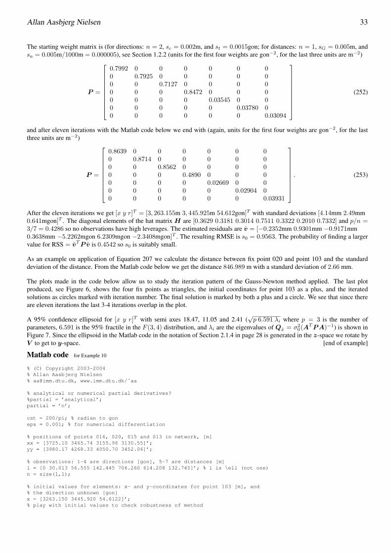
The starting weight matrix is (for directions: n = 2, sc = 0.002m, and st = 0.0015gon; for distances: n = 1, sG = 0.005m, andsa = 0.005m/1000m = 0.000005), see Section 1.2.2 (units for the first four weights are gon−2, for the last three units are m−2)

P =

0.7992 0 0 0 0 0 00 0.7925 0 0 0 0 00 0 0.7127 0 0 0 00 0 0 0.8472 0 0 00 0 0 0 0.03545 0 00 0 0 0 0 0.03780 00 0 0 0 0 0 0.03094

(252)

and after eleven iterations with the Matlab code below we end with (again, units for the first four weights are gon−2, for the lastthree units are m−2)

P =

0.8639 0 0 0 0 0 00 0.8714 0 0 0 0 00 0 0.8562 0 0 0 00 0 0 0.4890 0 0 00 0 0 0 0.02669 0 00 0 0 0 0 0.02904 00 0 0 0 0 0 0.03931

. (253)

After the eleven iterations we get [x y r]T = [3, 263.155m 3, 445.925m 54.612gon]T with standard deviations [4.14mm 2.49mm0.641mgon]T . The diagonal elements of the hat matrix H are [0.3629 0.3181 0.3014 0.7511 0.3322 0.2010 0.7332] and p/n =3/7 = 0.4286 so no observations have high leverages. The estimated residuals are v = [−0.2352mm 0.9301mm −0.9171mm0.3638mm −5.2262mgon 6.2309mgon −2.3408mgon]T . The resulting RMSE is s0 = 0.9563. The probability of finding a largervalue for RSS = vTP v is 0.4542 so s0 is suitably small.

As an example on application of Equation 207 we calculate the distance between fix point 020 and point 103 and the standarddeviation of the distance. From the Matlab code below we get the distance 846.989 m with a standard deviation of 2.66 mm.

The plots made in the code below allow us to study the iteration pattern of the Gauss-Newton method applied. The last plotproduced, see Figure 6, shows the four fix points as triangles, the initial coordinates for point 103 as a plus, and the iteratedsolutions as circles marked with iteration number. The final solution is marked by both a plus and a circle. We see that since thereare eleven iterations the last 3-4 iterations overlap in the plot.

A 95% confidence ellipsoid for [x y r]T with semi axes 18.47, 11.05 and 2.41 (√p 6.591 λi where p = 3 is the number of

parameters, 6.591 is the 95% fractile in the F (3, 4) distribution, and λi are the eigenvalues of Qx = σ20(A

TPA)−1) is shown inFigure 7. Since the ellipsoid in the Matlab code in the notation of Section 2.1.4 in page 28 is generated in the z-space we rotate byV to get to y-space. [end of example]

Matlab code for Example 10

% (C) Copyright 2003-2004% Allan Aasbjerg Nielsen% [email protected], www.imm.dtu.dk/˜aa

% analytical or numerical partial derivatives?%partial = ’analytical’;partial = ’n’;

cst = 200/pi; % radian to goneps = 0.001; % for numerical differentiation

% positions of points 016, 020, 015 and 013 in network, [m]xx = [3725.10 3465.74 3155.96 3130.55]’;yy = [3980.17 4268.33 4050.70 3452.06]’;

% observations: 1-4 are directions [gon], 5-7 are distances [m]l = [0 30.013 56.555 142.445 706.260 614.208 132.745]’; % l is \ell (not one)n = size(l,1);

% initial values for elements: x- and y-coordinates for point 103 [m], and% the direction unknown [gon]x = [3263.150 3445.920 54.6122]’;% play with initial values to check robustness of method


2.6 2.8 3 3.2 3.4 3.6 3.8 4

x 106

2.8

3

3.2

3.4

3.6

3.8

4

4.2

4.4x 10

6

103 start016

020

015

013

1

2

3

4

5

67

103 stop

x and y over iterations

Figure 6: Development of x and y coordinates of point 103 over iterations with first seven iterations annotated; righthandcoordinate system.

x = [0 0 -200]’;x = [0 0 -100]’;x = [0 0 100]’;x = [0 0 200]’;x = [0 0 40000]’;x = [0 0 0]’;x = [100000 100000 0]’;x = [mean(xx) mean(yy) 0]’;%x = [mean(xx) 3452.06 0]’; % approx. same y as 013p = size(x,1);

% desired units: mm and mgonxx = 1000*xx;yy = 1000*yy;l = 1000*l;x = 1000*x;cst = 1000*cst;

%number of degrees of freedomf = n-p;

x0 = x;

sc = 0.002*1000;%[mm]st = 0.0015*1000;%[mgon]sG = 0.005*1000;%[mm]sa = 0.000005;%[m/m], no unit%a [mm]

idx = [];e2 = [];dc = [];X = [];

for iter = 1:50 % iter ---------------------------------------------------------


−15−10

−50

510

15 −10

0

10

−2

0

2

y [mm]x [mm]

r [m

gon]

−15 −10 −5 0 5 10 15

−10

−5

0

5

10

x [mm]

y [m

m]

Figure 7: 95% ellipsoid for [x y r]T with projection on xy-plane.

% output from atan2 is in radian, convert to gonF1 = cst.*atan2(yy-x(2),xx-x(1))-x(3);a = (x(1)-xx).ˆ2+(x(2)-yy).ˆ2;F2 = sqrt(a);F = [F1; F2([1 3:end])]; % skip distance from 103 to 020

% weight matrix%a [mm]P = diag([2./(2*(cst*sc).ˆ2./a+stˆ2); 1./(sGˆ2+a([1 3:end])*sa.ˆ2)]);diag(P)’

k = l-F; % l is \ell (not one)

A1 = [];A2 = [];if strcmp(partial,’analytical’)

% A is matrix of analytical partial derivativeserror(’not implemented yet’);

else% A is matrix of numerical partial derivatives%directionsdF = (cst.*atan2(yy- x(2) ,xx-(x(1)+eps))- x(3) -F1)/eps;A1 = [A1 dF];dF = (cst.*atan2(yy-(x(2)+eps),xx- x(1) ) - x(3) -F1)/eps;A1 = [A1 dF];dF = (cst.*atan2(yy- x(2) ,xx- x(1) ) -(x(3)+eps)-F1)/eps;A1 = [A1 dF];%distancesdF = (sqrt((x(1)+eps-xx).ˆ2+(x(2) -yy).ˆ2)-F2)/eps;A2 = [A2 dF];dF = (sqrt((x(1) -xx).ˆ2+(x(2)+eps-yy).ˆ2)-F2)/eps;A2 = [A2 dF];dF = (sqrt((x(1) -xx).ˆ2+(x(2) -yy).ˆ2)-F2)/eps;A2 = [A2 dF];A2 = A2([1 3:4],:);% skip derivatives of distance from 103 to 020


A = [A1; A2];end

N = A’*P;c = N*k;N = N*A;%WLSdeltahat = N\c;khat = A*deltahat;vhat = k-khat;e2 = [e2 vhat’*P*vhat];dc = [dc deltahat’*c];%update for iterationsx = x+deltahat;X = [X x];

idx = [idx iter];

% stop iterationsitertst = (k’*P*k)/e2(end);if itertst < 1.000001

break;end

end % iter -------------------------------------------------------------------

%x-x0% number of iterationsiter

%MSEs02 = e2(end)/f;%RMSEs0 = sqrt(s02)

%Variance/covariance matrix of the observations, lDl = s02.*inv(P);%Standard deviationsstdl = sqrt(diag(Dl))

%Variance/covariance matrix of the adjusted elements, xhatNinv = inv(N);Dxhat = s02.*Ninv;%Standard deviationsstdxhat = sqrt(diag(Dxhat))

%Variance/covariance matrix of the adjusted observations, lhatDlhat = s02.*A*Ninv*A’;%Standard deviationsstdlhat = sqrt(diag(Dlhat))

%Variance/covariance matrix of the adjusted residuals, vhatDvhat = Dl-Dlhat;%Standard deviationsstdvhat = sqrt(diag(Dvhat))

%Correlations between adjusted elements, xhataux = diag(1./stdxhat);corrxhat = aux*Dxhat*aux

% Standard deviation of estimated distance from 103 to 020d020 = sqrt((xx(2)-x(1))ˆ2+(yy(2)-x(2))ˆ2);%numerical partial derivatives of d020, i.e. gradient of d020grad = [];dF = (sqrt((xx(2)-(x(1)+eps))ˆ2+(yy(2)- x(2) )ˆ2)-d020)/eps;grad = [grad; dF];dF = (sqrt((xx(2)- x(1) )ˆ2+(yy(2)-(x(2)+eps))ˆ2)-d020)/eps;grad = [grad; dF; 0];stdd020 = s0*sqrt(grad’*Ninv*grad)

% plots to illustrate progress of iterationsfigure%plot(idx,e2);semilogy(idx,e2);


title(’vˆTPv’);figure%plot(idx,dc);semilogy(idx,dc);title(’cˆTNˆ{-1}c’);figure%plot(idx,dc./e2);semilogy(idx,dc./e2);title(’(cˆTNˆ{-1}c)/(vˆTPv)’);for i = 1:p

figureplot(idx,X(i,:));%semilogy(idx,X(i,:));title(’X(i,:) vs. iteration index’);

endfigure%loglog(x0(1),x0(2),’k+’)plot(x0(1),x0(2),’k+’) % initial values for x and ytext(x0(1)+30000,x0(2)+30000,’103 start’)hold% positions of points 016, 020, 015 and 013 in network%loglog(xx,yy,’xk’)plot(xx,yy,’kˆ’)txt = [’016’; ’020’; ’015’; ’013’];for i = 1:4

text(xx(i)+30000,yy(i)+30000,txt(i,:));endfor i = 1:iter% loglog(X(1,i),X(2,i),’ko’);

plot(X(1,i),X(2,i),’ko’);endfor i = 1:7

text(X(1,i)+30000,X(2,i)-30000,num2str(i));endplot(X(1,end),X(2,end),’k+’);%loglog(X(1,end),X(2,end),’k+’);text(X(1,end)+30000,X(2,end)+30000,’103 stop’)title(’x and y over iterations’);%title(’X(1,:) vs. X(2,:) over iterations’);axis equalaxis([2.6e6 4e6 2.8e6 4.4e6])

% t-values and probabilities of finding larger |t|% pt should be smaller than, say, (5% or) 1%t = x./stdxhat;pt = betainc(f./(f+t.ˆ2),0.5*f,0.5);

% probabilitiy of finding larger v’Pv% should be greater than, say, 5% (or 1%)pchi2 = 1-gammainc(0.5*e2(end),0.5*f);

% semi-axes in confidence ellipsoid% 95% fractile for 3 dfs is 7.815 = 2.796ˆ2% 99% fractile for 3 dfs is 11.342 = 3.368ˆ2%[vDxhat dDxhat] = eigsort(Dxhat(1:2,1:2));[vDxhat dDxhat] = eigsort(Dxhat);%semiaxes = sqrt(diag(dDxhat));% 95% fractile for 2 dfs is 5.991 = 2.448ˆ2% 99% fractile for 2 dfs is 9.210 = 3.035ˆ2% df F(3,df).95 F(3,df).99% 1 215.71 5403.1% 2 19.164 99.166% 3 9.277 29.456% 4 6.591 16.694% 5 5.409 12.060% 10 3.708 6.552% 100 2.696 3.984% inf 2.605 3.781% chiˆ2 approximation, 95% fractilesemiaxes = sqrt(7.815*diag(dDxhat))figureellipsoidrot(0,0,0,semiaxes(1),semiaxes(2),semiaxes(3),vDxhat);axis equalxlabel(’x [mm]’); ylabel(’y [mm]’); zlabel(’r [mgon]’);


title(’95% confidence ellipsoid, \chiˆ2 approx.’)% F approximation, 95% fractile. NB the fractile depends on dfsemiaxes = sqrt(3*6.591*diag(dDxhat))figureellipsoidrot(0,0,0,semiaxes(1),semiaxes(2),semiaxes(3),vDxhat);axis equalxlabel(’x [mm]’); ylabel(’y [mm]’); zlabel(’r [mgon]’);title(’95% confidence ellipsoid, F approx.’)view(37.5,15)print -depsc2 confxyr.eps%clear%close all

function [v,d] = eigsort(a)[v1,d1] = eig(a);d2 = diag(d1);[dum,idx] = sort(d2);v = v1(:,idx);d = diag(d2(idx));

function [xx,yy,zz] = ellipsoidrot(xc,yc,zc,xr,yr,zr,Q,n)%ELLIPSOID Generate ellipsoid.%% [X,Y,Z] = ELLIPSOID(XC,YC,ZC,XR,YR,ZR,Q,N) generates three% (N+1)-by-(N+1) matrices so that SURF(X,Y,Z) produces a rotated% ellipsoid with center (XC,YC,ZC) and radii XR, YR, ZR.%% [X,Y,Z] = ELLIPSOID(XC,YC,ZC,XR,YR,ZR,Q) uses N = 20.%% ELLIPSOID(...) and ELLIPSOID(...,N) with no output arguments% graph the ellipsoid as a SURFACE and do not return anything.%% The ellipsoidal data is generated using the equation after rotation with% orthogonal matrix Q:%% (X-XC)ˆ2 (Y-YC)ˆ2 (Z-ZC)ˆ2% -------- + -------- + -------- = 1% XRˆ2 YRˆ2 ZRˆ2%% See also SPHERE, CYLINDER.

% Modified by Allan Aasbjerg Nielsen (2004) after% Laurens Schalekamp and Damian T. Packer% Copyright 1984-2002 The MathWorks, Inc.% $Revision: 1.7 $ $Date: 2002/06/14 20:33:49 $

error(nargchk(7,8,nargin));

if nargin == 7n = 20;end

[x,y,z] = sphere(n);

x = xr*x;y = yr*y;z = zr*z;xvec = Q*[reshape(x,1,(n+1)ˆ2); reshape(y,1,(n+1)ˆ2); reshape(z,1,(n+1)ˆ2)];x = reshape(xvec(1,:),n+1,n+1)+xc;y = reshape(xvec(2,:),n+1,n+1)+yc;z = reshape(xvec(3,:),n+1,n+1)+zc;if(nargout == 0)

surf(x,y,z)% surfl(x,y,z)% surfc(x,y,z)

axis equal%shading interp%colormap gray

elsexx = x;yy = y;zz = z;end


Example 11 In this example we have data on the positions of Navstar Global Positioning System (GPS)space vehicles (SV) 1, 4, 7, 13, 20, 24 and 25 and pseudoranges from our position to the SVs. We wantto determine the (3-D) coordinates [X Y Z]T of our position and the clock error in our GPS receiver, cdT ,[x1 x2 x3 x4]

T = [X Y Z cdT ]T , so the number of parameters is p = 4. The positions of and pseudoranges(ℓ) to the SVs given in a data file from the GPS receiver are

SV X [m] Y [m] Z [m] ℓ [m]1 16,577,402.072 5,640,460.750 20,151,933.185 20,432,524.04 11,793,840.229 –10,611,621.371 21,372,809.480 21,434,024.47 20,141,014.004 –17,040,472.264 2,512,131.115 24,556,171.0

13 22,622,494.101 –4,288,365.463 13,137,555.567 21,315,100.220 12,867,750.433 15,820,032.908 16,952,442.746 21,255,217.024 –3,189,257.131 –17,447,568.373 20,051,400.790 24,441,547.225 –7,437,756.358 13,957,664.984 21,692,377.935 23,768,678.3

.

The true position is (that of the no longer existing GPS station at Landmalervej in Hjortekær) [X Y Z]T =[3, 507, 884.948 780, 492.718 5, 251, 780.403]T m. We have seven observations, n = 7. Therefore we havef = n− p = 7− 4 = 3 degrees of freedom. The observation equations are (in m)

ℓ1 =√(16577402.072−X)2 + (5640460.750− Y )2 + (20151933.185− Z)2 + cdT + v1 (254)

ℓ2 =√(11793840.229−X)2 + (−10611621.371− Y )2 + (21372809.480− Z)2 + cdT + v2 (255)

ℓ3 =√(20141014.004−X)2 + (−17040472.264− Y )2 + (2512131.115− Z)2 + cdT + v3 (256)

ℓ4 =√(22622494.101−X)2 + (−4288365.463− Y )2 + (13137555.567− Z)2 + cdT + v4 (257)

ℓ5 =√(12867750.433−X)2 + (15820032.908− Y )2 + (16952442.746− Z)2 + cdT + v5 (258)

ℓ6 =√(−3189257.131−X)2 + (−17447568.373− Y )2 + (20051400.790− Z)2 + cdT + v6(259)

ℓ7 =√(−7437756.358−X)2 + (13957664.984− Y )2 + (21692377.935− Z)2 + cdT + v7 (260)

As the initial values [X∗ Y ∗ Z∗ cdT ∗]T we choose [0 0 0 0]T , center of the Earth, no clock error. First orderTaylor expansions of the observation equations near the initial values give (in m)

ℓ1 = d1 + cdT ∗ (261)

−16577402.072−X∗

d1∆X − 5640460.750− Y ∗

d1∆Y − 20151933.185− Z∗

d1∆Z +∆cdT + v1

ℓ2 = d2 + cdT ∗ (262)

−11793840.229−X∗

d2∆X − −10611621.371− Y ∗

d2∆Y − 21372809.480− Z∗

d2∆Z +∆cdT + v2

ℓ3 = d3 + cdT ∗ (263)

−20141014.004−X∗

d3∆X − −17040472.264− Y ∗

d3∆Y − 2512131.115− Z∗

d3∆Z +∆cdT + v3

ℓ4 = d4 + cdT ∗ (264)

−22622494.101−X∗

d4∆X − −4288365.463− Y ∗

d4∆Y − 13137555.567− Z∗

d4∆Z +∆cdT + v4

ℓ5 = d5 + cdT ∗ (265)

−12867750.433−X∗

d5∆X − 15820032.908− Y ∗

d5∆Y − 16952442.746− Z∗

d5∆Z +∆cdT + v5


ℓ6 = d6 + cdT ∗ (266)

−−3189257.131−X∗

d6∆X − −17447568.373− Y ∗

d6∆Y − 20051400.790− Z∗

d6∆Z +∆cdT + v6

ℓ7 = d7 + cdT ∗ (267)

−−7437756.358−X∗

d7∆X − 13957664.984− Y ∗

d7∆Y − 21692377.935− Z∗

d7∆Z +∆cdT + v7

where (in m)

d1 =√(16577402.072−X∗)2 + (5640460.750− Y ∗)2 + (20151933.185− Z∗)2 (268)

d2 =√(11793840.229−X∗)2 + (−10611621.371− Y ∗)2 + (21372809.480− Z∗)2 (269)

d3 =√(20141014.004−X∗)2 + (−17040472.264− Y ∗)2 + (2512131.115− Z∗)2 (270)

d4 =√(22622494.101−X∗)2 + (−4288365.463− Y ∗)2 + (13137555.567− Z∗)2 (271)

d5 =√(12867750.433−X∗)2 + (15820032.908− Y ∗)2 + (16952442.746− Z∗)2 (272)

d6 =√(−3189257.131−X∗)2 + (−17447568.373− Y ∗)2 + (20051400.790− Z∗)2 (273)

d7 =√(−7437756.358−X∗)2 + (13957664.984− Y ∗)2 + (21692377.935− Z∗)2. (274)

In matrix form we get (k = A∆; as above units are m)

20432524.0− d1 − cdT ∗

21434024.4− d2 − cdT ∗

24556171.0− d3 − cdT ∗

21315100.2− d4 − cdT ∗

21255217.0− d5 − cdT ∗

24441547.2− d6 − cdT ∗

23768678.3− d7 − cdT ∗

=

−16577402.072−X∗

d1−5640460.750−Y ∗

d1−20151933.185−Z∗

d11

−11793840.229−X∗

d2−−10611621.371−Y ∗

d2−21372809.480−Z∗

d21

−20141014.004−X∗

d3−−17040472.264−Y ∗

d3−2512131.115−Z∗

d31

−22622494.101−X∗

d4−−4288365.463−Y ∗

d4−13137555.567−Z∗

d41

−12867750.433−X∗

d5−15820032.908−Y ∗

d5−16952442.746−Z∗

d51

−−3189257.131−X∗

d6−−17447568.373−Y ∗

d6−20051400.790−Z∗

d61

−−7437756.358−X∗

d7−13957664.984−Y ∗

d7−21692377.935−Z∗

d71

∆X

∆Y

∆Z

∆cdT

.(275)

After five iterations with the Matlab code below (with all observations weighted equally, pi = 1/(10m)2)we get [X Y Z cdT ]T = [3, 507, 889.1 780, 490.0 5, 251, 783.8 25, 511.1]T m with standard deviations[6.42 5.31 11.69 7.86]T m. 25, 511.1 m corresponds to a clock error of 0.085 ms. The difference between thetrue position and the solution found is [−4.18 2.70 −3.35]T m, all well within one standard deviation. Thecorresponding distance is 6.00 m. Figure 8 shows the four parameters over the iterations including the startingguess. The diagonal elements of the hat matrix H are [0.4144 0.5200 0.8572 0.3528 0.4900 0.6437 0.7218]and p/n = 4/7 = 0.5714 so no observations have high leverages. The estimated residuals are v =[5.80 −5.10 0.74 −5.03 3.20 5.56 −5.17]T m. With prior variances of 102 m2, the resulting RMSE iss0 = 0.7149.

The probability of finding a larger value for RSS = vTP v is 0.6747 so s0 is suitably small. With prior variances of 52 m2 insteadof 102 m2, s0 is 1.4297 and the probability of finding a larger value for RSS = vTP v is 0.1054 so also in this situation s0 issuitably small. With prior variances of 32 m2 instead of 102 m2, s0 is 2.3828 and the probability of finding a larger value forRSS = vTP v is 0.0007 so in this situation s0 is too large.

95% confidence ellipsoids for [X Y Z]T in an earth-centered-earth-fixed (ECEF) coordinate system and in a local Easting-Northing-Up (ENU) coordinate system are shown in Figure 9. The semi axes in both the ECEF and the ENU systems are 64.92,30.76 and 23.96 (this is

√m 9.277 λi where m = 3 is the number of parameters, 9.277 is the 95% fractile in the F (3, 3) distribu-

tion, and λi are the eigenvalues of QXY Z , the upper-left 3× 3 submatrix of Qx = σ20(A

TPA)−1); units are metres. The rotationto the local ENU system is performed by means of the orthogonal matrix (F TF = FF T = I)

F T =

− sinλ cosλ 0− sinϕ cosλ − sinϕ sinλ cosϕcosϕ cosλ cosϕ sinλ sinϕ

(276)


0 50

2

4

6x 10

6

0 50

5

10x 10

5

0 50

2

4

6

8x 10

6

0 50

5

10

15x 10

5

Figure 8: Parameters [X Y Z cdT ]T over iterations including the starting guess.

where ϕ is the latitude and λ is the longitude. The variance-covariance matrix of the position estimates in the ENU coordinatesystem is QENU = F TQXY ZF . Since

QXY Za = λa (277)F TQXY ZFF Ta = λF Ta (278)

QENU (FTa) = λ(F Ta) (279)

we see that QXY Z and QENU have the same eigenvalues and their eigenvectors are related as indicated. Since the ellipsoid in theMatlab code in the notation of Section 2.1.4 in page 28 is generated in the z-space we rotate by V to get to y-space.

Dilution of Precision, DOP Satellite positioning works best when there is a good angular separation between the space vehicles.A measure of this separation is termed the dilution of precision, DOP. Low values of the DOP correspond to a good angularseparation, high values to a bad angular separation, i.e., a high degree of clustering of the SVs. There are several versions of DOP.From Equation 193 the dispersion of the parameters is

Qx = D{xWLS} = σ20(A

TPA)−1. (280)

This matrix has contributions from our prior expectations to the precision of the measurements (P ), the actual precision of themeasurements (σ2

0) and the geometry of the problem (A). Let’s look at the geometry alone and define the symmetric matrix

QDOP = Qx/(σ20 σ2

prior) = (ATPA)−1/σ2prior =

q2X qXY qXZ qXcdT

qXY q2Y qY Z qY cdT

qXZ qY Z q2Z qZcdT

qXcdT qY cdT qZcdT q2cdT

(281)

where σ2prior = σ2

i,prior, i.e., all prior variances are equal, see Section 1.2.2. In WLS (with equal weights on all observations) thiscorresponds to QDOP = (ATA)−1.

We are now ready to define the position DOP

PDOP =√

q2X + q2Y + q2Z , (282)

the time DOP

TDOP =√q2cdT = qcdT (283)

and the geometric DOP

GDOP =√q2X + q2Y + q2Z + q2cdT (284)

which is the square root of the trace of QDOP . It is easily seen that GDOP 2 = PDOP 2 + TDOP 2.

In practice PDOP values less than 2 are considered excellent, between 2 and 4 good, up to 6 acceptable. PDOP values greater thanaround 6 are considered suspect.

DOP is a measure of size of the matrix QDOP (or sub-matrices thereof, for PDOP for example the upper left three by three matrix).As an alternative measure of this size we could use the determinant. Such a DOP measure would allow for off-diagonal elements


of QDOP , i.e., for covariances between the final estimates of the position. Determinant based DOP measures are not used in theGNSS literature.

After rotation from the ECEF to the ENU coordinate system which transforms the upper-left 3 × 3 submatrix QXY Z of Qx intoQENU , we can define

QDOP,ENU = QENU/(σ20 σ2

prior) =

q2E qEN qEU

qEN q2N qNU

qEU qNU q2U

, (285)

the horizontal DOP

HDOP =√

q2E + q2N (286)

and the vertical DOP

V DOP =√

q2U = qU . (287)

We see that PDOP 2 = HDOP 2 + V DOP 2 which is the trace of QDOP,ENU . [end of example]

−200

20

−200

20

−60

−40

−20

0

20

40

60

X [m]Y [m]

Z [m

]

−200

20−20

020

−60

−40

−20

0

20

40

60

E [m]N [m]

U [m

]

−20 0 20

−30

−20

−10

0

10

20

30

E [m]

N [m

]

Figure 9: 95% ellipsoid for [X Y Z]T in ECEF (left) and ENU (middle) coordinate systems with projection on EN-plane (right).

Matlab code for Example 11Code for functions eigsort and ellipsoidrot are listed under Example 10.


format short g

% use analytical partial derivativespartial = ’analytical’;%partial = ’n’;% speed of light, [m/s]%clight = 300000000;clight = 299792458;% length of C/A code, [m]%L = 300000;

% true position (Landmaalervej, Hjortekaer)xtrue = [3507884.948 780492.718 5251780.403 0]’;% positions of satellites 1, 4, 7, 13, 20, 24 and 25 in ECEF coordinate system, [m]


xxyyzz = [16577402.072 5640460.750 20151933.185;11793840.229 -10611621.371 21372809.480;20141014.004 -17040472.264 2512131.115;22622494.101 -4288365.463 13137555.567;12867750.433 15820032.908 16952442.746;-3189257.131 -17447568.373 20051400.790;-7437756.358 13957664.984 21692377.935];

pseudorange = [20432524.0 21434024.4 24556171.0 21315100.2 21255217.0 ...24441547.2 23768678.3]’; % [m]

l = pseudorange; % l is \ell (not one)xx = xxyyzz(:,1);yy = xxyyzz(:,2);zz = xxyyzz(:,3);n = size(xx,1); % number of observations

% weight matrixsprior2 = 10ˆ2; %5ˆ2; %prior variance [mˆ2]P = eye(n)/sprior2; % weight = 1/"prior variance" [mˆ(-2)]

% preliminary position, [m]x = [0 0 0 0]’;p = size(x,1); % number of elements/parametersf = n-p; % number of degrees of freedomx0 = x;

for iter = 1:20 % iter --------------------------------------------------------------

range = sqrt((x(1)-xx).ˆ2+(x(2)-yy).ˆ2+(x(3)-zz).ˆ2);prange = range+x(4);F = prange;

A = [];if strcmp(partial,’analytical’)

% A is matrix of analytical partial derivativesirange = 1./range;dF = irange.*(x(1)-xx);A = [A dF];dF = irange.*(x(2)-yy);A = [A dF];dF = irange.*(x(3)-zz);A = [A dF];dF = ones(n,1);A = [A dF];

else% A is matrix of numerical partial derivativesdF = sqrt((x(1)+1-xx).ˆ2+(x(2) -yy).ˆ2+(x(3) -zz).ˆ2)+ x(4) -prange;A = [A dF];dF = sqrt((x(1) -xx).ˆ2+(x(2)+1-yy).ˆ2+(x(3) -zz).ˆ2)+ x(4) -prange;A = [A dF];dF = sqrt((x(1) -xx).ˆ2+(x(2) -yy).ˆ2+(x(3)+1-zz).ˆ2)+ x(4) -prange;A = [A dF];dF = sqrt((x(1) -xx).ˆ2+(x(2) -yy).ˆ2+(x(3) -zz).ˆ2)+(x(4)+1)-prange;A = [A dF];

end

k = l-F; % l is \ell (not one)%k = -l+F;N = A’*P;c = N*k;N = N*A;deltahat = N\c;% OLS solution%deltahat = A\k;% WLS-as-OLS solution%sqrtP = sqrt(P);%deltahat = (sqrtP*A)\(sqrtP*k)

khat = A*deltahat;vhat = k-khat;

% prepare for iterationsx = x+deltahat;

% stop iterations


if max(abs(deltahat))<0.001break

end%itertst = (k’*P*k)/(vhat’*P*vhat);%if itertst < 1.000001% break%end

end % iter --------------------------------------------------------------

% DOPSSE = vhat’*P*vhat; %RSS or SSEs02 = SSE/f; % MSEs0 = sqrt(s02); %RMSEQdop = inv(A’*P*A);Qx = s02.*Qdop;Qdop = Qdop/sprior2;PDOP = sqrt(trace(Qdop(1:3,1:3)));% must be in local Easting-Northing-Up coordinates%HDOP = sqrt(trace(Qdop(1:2,1:2)));% must be in local Easting-Northing-Up coordinates%VDOP = sqrt(Qdop(3,3));TDOP = sqrt(Qdop(4,4));GDOP = sqrt(trace(Qdop));

% Dispersion etc of elements%Qx = s02.*inv(A’*P*A);sigmas = sqrt(diag(Qx));sigma = diag(sigmas);isigma = inv(sigma);% correlations between estimatesRx = isigma*Qx*isigma;

% Standardised residuals%Qv = s02.*(inv(P)-A*inv(A’*P*A)*A’);Qv = s02.*inv(P)-A*Qx*A’;sigmares = sqrt(diag(Qv));stdres = vhat./sigmares;

disp(’----------------------------------------------------------’)disp(’estimated parameters/elements [m]’)xdisp(’estimated clock error [s]’)x(4)/clightdisp(’number of iterations’)iterdisp(’standard errors of elements [m]’)sigmas%tval = x./sigmasdisp(’s0’)s0disp(’PDOP’)PDOP%stdresdisp(’difference between estimated elements and initial guess’)deltaori = x-x0disp(’difference between true values and estimated elements’)deltaori = xtrue-xdisp(’----------------------------------------------------------’)

% t-values and probabilities of finding larger |t|% pt should be smaller than, say, (5% or) 1%t = x./sigmas;pt = betainc(f./(f+t.ˆ2),0.5*f,0.5);

% probabilitiy of finding larger s02% should be greater than, say, 5% (or 1%)pchi2 = 1-gammainc(0.5*SSE,0.5*f);

% semi-axes in confidence ellipsoid for position estimates% 95% fractile for 3 dfs is 7.815 = 2.796ˆ2% 99% fractile for 3 dfs is 11.342 = 3.368ˆ2[vQx dQx] = eigsort(Qx(1:3,1:3));semiaxes = sqrt(diag(dQx));


% 95% fractile for 2 dfs is 5.991 = 2.448ˆ2% 99% fractile for 2 dfs is 9.210 = 3.035ˆ2

% df F(3,df).95 F(3,df).99% 1 215.71 5403.1% 2 19.164 99.166% 3 9.277 29.456% 4 6.591 16.694% 5 5.409 12.060% 10 3.708 6.552% 100 2.696 3.984% inf 2.605 3.781% chiˆ2 approximation, 95% fractilefigureellipsoidrot(0,0,0,semiaxes(1)*sqrt(7.815),semiaxes(2)*sqrt(7.815),...

semiaxes(3)*sqrt(7.815),vQx);axis equalxlabel(’X [m]’); ylabel(’Y [m]’); zlabel(’Z [m]’);title(’95% confidence ellipsoid, ECEF, \chiˆ2 approx.’)% F approximation, 95% fractile. NB the fractile depends on dffigureellipsoidrot(0,0,0,semiaxes(1)*sqrt(3*9.277),semiaxes(2)*sqrt(3*9.277),...

semiaxes(3)*sqrt(3*9.277),vQx);axis equalxlabel(’X [m]’); ylabel(’Y [m]’); zlabel(’Z [m]’);title(’95% confidence ellipsoid, ECEF, F approx.’)print -depsc2 confXYZ.eps%% F approximation; number of obs goes to infinity%figure%ellipsoidrot(0,0,0,semiaxes(1)*sqrt(3*2.605),semiaxes(2)*sqrt(3*2.605),...% semiaxes(3)*sqrt(3*2.605),vQx);%axis equal%xlabel(’X [m]’); ylabel(’Y [m]’); zlabel(’Z [m]’);%title(’95% confidence ellipsoid, ECEF, F approx., nobs -> inf’)

% To geographical coordinates, from Strang & Borre (1997)[bb,ll,hh,phi,lambda] = c2gwgs84(x(1),x(2),x(3))

% Convert Qx (ECEF) to Qenu (ENU)sp = sin(phi);cp = cos(phi);sl = sin(lambda);cl = cos(lambda);Ft = [-sl cl 0; -sp*cl -sp*sl cp; cp*cl cp*sl sp]; % ECEF -> ENUQenu = Ft*Qx(1:3,1:3)*Ft’;% std.err. of ENUsigmasenu = sqrt(diag(Qenu));[vQenu dQenu] = eigsort(Qenu(1:3,1:3));semiaxes = sqrt(diag(dQenu));

% F approximation, 95% fractile. NB the fractile depends on dffigureellipsoidrot(0,0,0,semiaxes(1)*sqrt(3*9.277),semiaxes(2)*sqrt(3*9.277),...

semiaxes(3)*sqrt(3*9.277),vQenu);axis equalxlabel(’E [m]’); ylabel(’N [m]’); zlabel(’U [m]’);title(’95% confidence ellipsoid, ENU, F approx.’)print -depsc2 confENU.eps% Same thing, only more elegantfigureellipsoidrot(0,0,0,semiaxes(1)*sqrt(3*9.277),semiaxes(2)*sqrt(3*9.277),...

semiaxes(3)*sqrt(3*9.277),Ft*vQx);axis equalxlabel(’E [m]’); ylabel(’N [m]’); zlabel(’U [m]’);title(’95% confidence ellipsoid, ENU, F approx.’)

%PDOP = sqrt(trace(Qenu)/sprior2)/s0;HDOP = sqrt(trace(Qenu(1:2,1:2))/sprior2)/s0;VDOP = sqrt(Qenu(3,3)/sprior2)/s0;

% Studentized/jackknifed residualsif f>1 studres = stdres./sqrt((f-stdres.ˆ2)/(f-1));end


function [bb,ll,h,phi,lambda] = c2gwgs84(x,y,z)

% C2GWGS84% Convertion of cartesian coordinates (X,Y,Z) to geographical% coordinates (phi,lambda,h) on the WGS 1984 reference ellipsoid%% phi and lambda are output as vectors: [degrees minutes seconds]’

% Modified by Allan Aasbjerg Nielsen (2004) after% Kai Borre 02-19-94% Copyright (c) by Kai Borre% $Revision: 1.0 $ $Date: 1997/10/15 %

a = 6378137;f = 1/298.257223563;

lambda = atan2(y,x);ex2 = (2-f)*f/((1-f)ˆ2);c = a*sqrt(1+ex2);phi = atan(z/((sqrt(xˆ2+yˆ2)*(1-(2-f))*f)));

h = 0.1; oldh = 0;while abs(h-oldh) > 1.e-12

oldh = h;N = c/sqrt(1+ex2*cos(phi)ˆ2);phi = atan(z/((sqrt(xˆ2+yˆ2)*(1-(2-f)*f*N/(N+h)))));h = sqrt(xˆ2+yˆ2)/cos(phi)-N;

end

phi1 = phi*180/pi;b = zeros(1,3);b(1) = fix(phi1);b(2) = fix(rem(phi1,b(1))*60);b(3) = (phi1-b(1)-b(2)/60)*3600;bb = [b(1) b(2) b(3)]’;lambda1 = lambda*180/pi;l = zeros(1,3);l(1) = fix(lambda1);l(2) = fix(rem(lambda1,l(1))*60);l(3) = (lambda1-l(1)-l(2)/60)*3600;ll = [l(1) l(2) l(3)]’;

2.2 Nonlinear WLS by other Methods

The remaining sections describe a few other methods often used for solving the nonlinear (weighted) least squares regressionproblem.

2.2.1 The Gradient or Steepest Descent Method

Let us go back to Equation 168: yi = fi(θ) + ei, i = 1, . . . , n and consider the nonlinear WLS case

∥e2(θ)∥ = eTPe/2 =1

2

n∑i=1

pi[yi − fi(θ)]2. (288)

The components of the gradient ∇∥e2∥ are

∂∥e2∥∂θk

= −n∑

i=1

pi[yi − fi(θ)]∂fi(θ)

∂θk. (289)

From an initial value (an educated guess) we can update θ by taking a step in the direction in which ∥e2∥ decreases most rapidly,namely in the direction of the negative gradient

θnew = θold − α∇∥e2(θold)∥ (290)

where α > 0 determines the step size. This is done iteratively until convergence.


2.2.2 Newton’s Method

Let us now expand ∥e2(θ)∥ to second order around an initial value θ0

∥e2(θ)∥ ≃ ∥e2(θ0)∥+ [∇∥e2(θ0)∥]T (θ − θ0) +1

2[θ − θ0]

TH(θ0)[θ − θ0] (291)

where H = ∂2∥e2(θ)∥/∂θ∂θT is the second order derivative of ∥e2(θ)∥ also known as the Hessian matrix not to be confusedwith the hat matrix in Equations 44, 114 and 196. The gradient of the above expansion is

∇∥e2(θ)∥ ≃ ∇∥e2(θ0)∥+H(θ0)[θ − θ0]. (292)

At the minimum ∇∥e2(θ)∥ = 0 and therefore we can find that minimum by updating

θnew = θold −H−1old∇∥e2(θold)∥ (293)

until convergence.

From Equation 289 the elements of the Hessian H are

Hkl =∂2∥e2∥∂θk∂θl

=n∑

i=1

pi

[∂fi(θ)

∂θk

∂fi(θ)

∂θl− [yi − fi(θ)]

∂2fi(θ)

∂θk∂θl

]. (294)

We see that the Hessian is symmetric. The second term in Hkl depends on the sum of the residuals between model and data,which is supposedly small both since our model is assumed to be good and since its terms can have opposite signs. It is thereforecustomary to omit this term. If the Hessian is positive definite we have a local minimizer and if its negative definite we have a localmaximizer (if its indefinite, i.e., it has both positive and negative eigenvalues, we have a saddle point). H is sometimes termed thecurvature matrix.

2.2.3 The Gauss-Newton Method

The basis of the Gauss-Newton method is a linear Taylor expansion of e

e(θ) ≃ e(θ0) + J(θ0)[θ − θ0] (295)

where J is the so-called Jacobian matrix containing the partial derivatives of e (like A containing the partial derivatives of F inEquation 179). In the WLS case this leads to

1

2eT (θ)Pe(θ) ≃ 1

2eT (θ0)Pe(θ)0 + [θ − θ0]

TJT (θ0)Pe(θ0) +1

2[θ − θ0]

TJT (θ0)PJ(θ0)[θ − θ0]. (296)

The gradient of this expression is JT (θ0)Pe(θ0) + JT (θ0)PJ(θ0)[θ − θ0] and its Hessian is JT (θ0)PJ(θ0). The gradientevaluated at θ0 is JT (θ0)Pe(θ0). We see that the Hessian is independent of θ − θ0, it is symmetric and it is positive definite ifJ(θ0) is full rank corresponding to linearly independent columns. Since the Hessian is positive definite we have a minimizer andsince ∇∥e2(θold)∥ = JT (θold)Pe(θold) we get from Equation 293

θnew = θold − [JT (θold)PJ(θold)]−1JT (θold)Pe(θold). (297)

This corresponds to the normal equations for θnew − θold

[JT (θold)PJ(θold)](θnew − θold) = −JT (θold)Pe(θold). (298)

This is equivalent to Equation 181 so the linearization method described in Section 2.1 is actually the Gauss-Newton method with−A as the Jacobian.

It can be shown that if the function to be minimized is twice continuously differentiable in a neighbourhood around the solutionθ∗, if J(θ) over iterations is nonsingular, and if the initial solution θ0, is close enough to θ∗, then the Gauss-Newton methodconverges. It can also be shown that the convergence is quadratic, i.e., the length of the increment vector (∆ in Section 2.1 and hin the Matlab function below) decreases quadratically over iterations.

Below is an example of a Matlab function implementation of the unweighted version of the Gauss-Newton algorithm. Note, thatthe code to solve the positioning problem is a while loop the body of which is three (or four) statements only. This is easilyextended with the weighting and the statistics part given in the previous example (do this as an exercise). Note also, that in the callto function gaussnewton we need to call the function fJ with the at symbol (@) to create a Matlab function handle.


Matlab code for Example 11

function x = gaussnewton(fJ, x0, tol, itermax)

% x = gaussnewton(@fJ, x0, tol, itermax)%% gaussnewton solves a system of nonlinear equations% by the Gauss-Newton method.%% fJ - gives f(x) and the Jacobian J(x) by [f, J] = fJ(x)% x0 - initial solution% tol - tolerance, iterate until maximum absolute value of correction% is smaller than tol% itermax - maximum number of iterations%% x - final solution%% fJ is written for the occasion

% (c) Copyright 2005% Allan Aasbjerg Nielsen% [email protected], www.imm.dtu.dk/˜aa% 8 Nov 2005

% Modified after% L. Elden, L. Wittmeyer-Koch and H.B. Nielsen (2004).

if nargin < 2, error(’too few input arguments’); endif nargin < 3, tol = 1e-2; endif nargin < 4, itermax = 100; end

iter = 0;x = x0;h = realmax*ones(size(x0));

while (max(abs(h)) > tol) && (iter < itermax)[f, J] = feval(fJ, x);h = J\f;x = x - h;iter = iter + 1;

end

%%%%%%%%%%%%%%%%%%%%%%%%%%%%%%%%%%%%%%%%%%%%%%%%%%%%%%%%%%%%%%

function [f, J] = fJ(x)

xxyyzz = [16577402.072 5640460.750 20151933.185;11793840.229 -10611621.371 21372809.480;20141014.004 -17040472.264 2512131.115;22622494.101 -4288365.463 13137555.567;12867750.433 15820032.908 16952442.746;-3189257.131 -17447568.373 20051400.790;-7437756.358 13957664.984 21692377.935]; % [m]

l = [20432524.0 21434024.4 24556171.0 21315100.2 21255217.0 24441547.2 ...23768678.3]’; % [m]

xx = xxyyzz(:,1);yy = xxyyzz(:,2);zz = xxyyzz(:,3);

range = sqrt((x(1)-xx).ˆ2 + (x(2)-yy).ˆ2 + (x(3)-zz).ˆ2);prange = range + x(4);f = l - prange;

if nargout < 2, return; end

n = size(f,1); % # obsp = 4; % # parametersJ = zeros(n,p);

% analytical derivativesJ(:,1) = -(x(1)-xx)./range;J(:,2) = -(x(2)-yy)./range;J(:,3) = -(x(3)-zz)./range;J(:,4) = -ones(n,1);


return

% numerical derivativesdelta = 1;for i = 1:p

y = x;y(i) = x(i) + delta;J(:,i) = (fJ(y) - f); %./delta;

end

return

% or symmetrizeddelta = 0.5;for i = 1:p

y = x;z = x;y(i) = x(i) + delta;z(i) = x(i) - delta;J(:,i) = (fJ(y) - fJ(z)); %./(2*delta);

end

2.2.4 The Levenberg-Marquardt Method

The Gauss-Newton method may cause the new θ to wander off further from the minimum than the old θ because of nonlinear com-ponents in e which are not modelled. Near the minimum the Gauss-Newton method converges very rapidly whereas the gradientmethod is slow because the gradient vanishes at the minimum. In the Levenberg-Marquardt method we modify Equation 298 to

[JT (θold)PJ(θold) + µI](θnew − θold) = −JT (θold)Pe(θold) (299)

where µ ≥ 0 is termed the damping factor. The Levenberg-Marquardt method is a hybrid of the gradient method far from theminimum and the Gauss-Newton method near the minimum: if µ is large we step in the direction of the steepest descent, if µ = 0we have the Gauss-Newton method.

Also Newton’s method may cause the new θ to wander off further from the minimum than the old θ since the Hessian may beindefinite or even negative definite (this is not the case for JTPJ ). In a Levenberg-Marquardt-like extension to Newton’s methodwe could modify Equation 293 to

θnew = θold − (Hold + µI)−1∇∥e2(θold)∥. (300)

3 Final Comments

In geodesy (and land surveying and GNSS) applications of regression analysis we are often interested inthe estimates of the regression coefficients also known as the parameters or the elements which are often2- or 3-D geographical positions, and their estimation accuracies. In many other application areas we are(also) interested in the ability of the model to predict values of the response variable from new values of theexplanatory variables not used to build the model.

Unlike the Gauss-Newton method both the gradient method and Newton’s method are general and not re-stricted to least squares problems, i.e., the functions to be optimized are not restricted to the form eTe oreTPe. Many other methods than the ones described and sketched here both general and least squares meth-ods such as quasi-Newton methods, conjugate gradients and simplex search methods exist.

Solving the problem of finding a global optimum in general is very difficult. The methods described andsketched here (and many others) find a minimum that depends on the set of initial values chosen for theparameters to estimate. This minimum may be local. It is often wise to use several sets of initial values tocheck the robustness of the solution offered by the method chosen.


Literature

P.R. Bevington (1969). Data Reduction and Error Analysis for the Physical Sciences. McGraw-Hill.

K. Borre (1990). Landmaling. Institut for Samfundsudvikling og Planlægning, Aalborg. In Danish.

K. Borre (1992). Mindste Kvadraters Princip Anvendt i Landmalingen. Aalborg. In Danish.

M. Canty, A.A. Nielsen and M. Schmidt (2004). Automatic radiometric normalization of multitemporalsatellite imagery. Remote Sensing of Environment 41(1), 4-19.

P. Cederholm (2000). Udjævning. Aalborg Universitet. In Danish.

R.D. Cook and S. Weisberg (1982). Residuals and Infuence in Regression. Chapman & Hall.

K. Conradsen (1984). En Introduktion til Statistik, vol. 1A-2B. Informatik og Matematisk Modellering, Dan-marks Tekniske Universitet. In Danish.

K. Dueholm, M. Laurentzius and A.B.O. Jensen (2005). GPS. 3rd Edition. Nyt Teknisk Forlag. In Danish.

L. Elden, L. Wittmeyer-Koch and H.B. Nielsen (2004). Introduction to Numerical Computation - analysisand MATLAB illustrations. Studentlitteratur.

N. Gershenfeld (1999). The Nature of Mathematical Modeling.

Cambridge University Press.

G.H. Golub and C.F. van Loan (1996). Matrix Computations, Third Edition. Johns Hopkins University Press.

P.S. Hansen, M.P. Bendsøe and H.B. Nielsen (1987). Lineær Algebra - Datamatorienteret. Informatik ogMatematisk Modellering, Matematisk Institut, Danmarks Tekniske Universitet. In Danish.

T. Hastie, R. Tibshirani and J. Friedman (2009). The Elements of Statistical Learning: Data Mining, Infer-ence, and Prediction. Second Edition. Springer.

O. Jacobi (1977). Landmaling 2. del. Hovedpunktsnet. Den private Ingeniørfond, Danmarks Tekniske Uni-versitet. In Danish.

A.B.O. Jensen (2002). Numerical Weather Predictions for Network RTK. Publication Series 4, volume 10.National Survey and Cadastre, Denmark.

N. Kousgaard (1986). Anvendt Regressionsanalyse for Samfundsvidenskaberne. Akademisk Forlag. In Dan-ish.

K. Madsen, H.B. Nielsen and O. Tingleff (1999). Methods for Non-Linear Least Squares Problems. Infor-matics and Mathematical Modelling, Technical University of Denmark.

P. McCullagh and J. Nelder (1989). Generalized Linear Models. Chapman & Hall. London, U.K.

E.M. Mikhail, J.S. Bethel and J.C. McGlone (2001). Introduction to Modern Photogrammetry. John Wileyand Sons.

E. Mærsk-Møller and P. Frederiksen (1984). Landmaling: Elementudjævning. Den private Ingeniørfond,Danmarks Tekniske Universitet. In Danish.


A.A. Nielsen (2001). Spectral mixture analysis: linear and semi-parametric full and partial unmixing inmulti- and hyperspectral image data. International Journal of Computer Vision 42(1-2), 17-37 and Journalof Mathematical Imaging and Vision 15(1-2), 17-37.

W.H. Press, S.A. Teukolsky, W.T. Vetterling and B.P. Flannery (1992). Numerical Recipes in C: The Art ofScientific Computing. Second Edition. Cambridge University Press.

J.A. Rice (1995). Mathematical Statistics and Data Analysis. Second Edition. Duxbury Press.

G. Strang (1980). Linear Algebra and its Applications. Second Edition. Academic Press.

G. Strang and K. Borre (1997). Linear Algebra, Geodesy, and GPS. Wellesley-Cambridge Press.

P. Thyregod (1998). En Introduktion til Statistik, vol. 3A-3D. Informatik og Matematisk Modellering, Dan-marks Tekniske Universitet. In Danish.

W.N. Venables and B.D. Ripley (1999). Modern Applied Statistics with S-PLUS. Third Edition. Springer.

IndexF distribution, 28R2, 12χ2 distribution, 21, 23, 28σ0, 16, 18s0, 21, 28t distribution, 12, 13, 22t-test, two-sided, 12, 22

adjustment, 7

chain rule, 29, 30Cholesky, 8, 15–17, 23, 27coefficient of determination, 12confidence

ellipsoid, 28, 33, 41Cook’s distance, 14coordinate system

ECEF, 41ENU, 41

damping factor, 49decomposition

Cholesky, 15QR, 15singular value, 15

degrees of freedom, 7derivative matrix, 26, 29dilution of precision, 41dispersion matrix, 11, 21, 27distribution

F , 28χ2, 21, 23, 28t, 12, 13, 22normal, 12, 21, 22

DOP, 41

ECEF coordinate system, 41ENU coordinate system, 41error

ellipsoid, 28gross, 13or residual, 6, 7

estimatorcentral, 9, 18unbiased, 9, 18

fundamental equations, 9, 17, 26

Gauss-Newton method, 27, 33, 47, 48, 50Global Navigation Satellite System, 29, 31Global Positioning System, 39GNSS, 29, 31

GPS, 39gradient method, 47

hat matrix, 9, 17Hessian, 47–49

idempotent, 9, 17iid, 12influence, 11, 14, 28initial value, 25, 29, 47, 50iterations, 27iterative solution, 27

Jacobian, 27, 47, 48

least squaresgeneral (GLS), 24nonlinear (NLS), 24ordinary (OLS), 7weighted (WLS), 16WLS as OLS, 24

levelling, 19Levenberg-Marquardt method, 49leverage, 11, 14, 21, 28, 33, 40linear constraints, 8, 26linearization, 25, 26

Matlab command mldivide, 13minimum

global, 50local, 50

MSE, 11, 21, 28multicollinearity, 8, 17, 27multiple regression, 6

Navstar, 39Newton’s method, 47, 50normal distribution, 12, 21, 22normal equations, 8, 17, 24

objective function, 7, 16observation equations, 7, 26optimum

global, 50local, 50

orientation unknown, 30, 31outlier, 13, 14

partial derivativesanalytical, 29numerical, 30

precision

52


dilution of, 41pseudorange, 39

QR, 8, 13, 15, 17, 27

regression, 7multiple, 6simple, 4

regressors, 6residual

jackknifed, 13or error, 6standardized, 13studentized, 13

RMSE, 11, 21, 28RSS, 11, 21, 27

significance, 12, 22, 28simple regression, 4space vehicle, 31, 39SSE, 11, 21, 27standard deviation of unit weight, 16steepest descent method, 47SVD, 8, 15, 17, 27

Taylor expansion, 25, 29, 47

uncertainty, 7

variabledependent, 6explanatory, 6independent, 6predictor, 6response, 6

variance-covariance matrix, 11, 21, 27

weights, 18

least squares adjustment: linear and nonlinear weighted regression...

Documents