Least squares estimation of nonlinear spatial trends

Rosa M. CRUJEIRAS ∗ Ingrid VAN KEILEGOM †

Abstract

The goal of this work is to study the asymptotic and finite sample properties of an

estimator of a nonlinear regression function when errors are spatially correlated, and

when the spatial dependence structure is unknown. The proposed method is based on

a weighted nonlinear least squares approach, taking into account the spatial covari-

ance. Weak consistency of the regression parameters estimator is derived, along with

its asymptotic Gaussian limit. The behavior of the proposed estimator is illustrated

with a simulation study, considering different correlation structures in R2 and a more

general case including a spatial covariate. The method is also applied to two real data

cases.

Key words and phrases. Asymptotic normality; Nonlinear least squares; Spatial regression;

Variogram.

∗Institute of Statistics, Universite catholique de Louvain, Voie du Roman Pays 20, B 1348 Louvain-la-

Neuve, Belgium. E-mail address: rosa.crujeiras@usc.es. Research supported by IAP research net-

work grant nr. P6/03 of the Belgian government (Belgian Science Policy) and Xunta de Galicia Project

PGIDIT06PXIB207009PR.†Institute of Statistics, Universite catholique de Louvain, Voie du Roman Pays 20, B 1348 Louvain-

la-Neuve, Belgium. E-mail address: ingrid.vankeilegom@uclouvain.be. Research supported by IAP

research network grant nr. P6/03 of the Belgian government (Belgian Science Policy), and by the European

Research Council under the European Community’s Seventh Framework Programme (FP7/2007-2013) /

ERC Grant agreement No. 203650.

1

1 Introduction

Consider a regression model Y (s) = g(s) + ε(s), where s belongs to some subset of Rd.The errors ε(s) are assumed to be spatially correlated, but we do not impose any type of

structural condition. We are mostly interested in the case where d = 2 (spatial setting) or

d = 3 (spatio-temporal setting), but other values of d are also possible. Spatial locations

may be irregularly spaced. In this paper we suppose that the regression function g belongs

to some parametric class gθ : θ ∈ Θ of (nonlinear) functions, and we are interested in the

estimation of the parameters of this model, when the error correlation structure is unknown.

Nonlinear trends are present in many examples involving spatially dependent data. For

instance, in soil science, [21] describe a sigmoide growth curve for modelling the relation-

ship between irrigation and soil water content; in environmental science, [15] considers a

nonlinear trend model for sulphate deposition, and in meteorology, [24] derives a nonlinear

model for acid deposition, based on a differential equation system.

In the context of nonlinear regression with time-dependent errors, [11] consider the esti-

mation of a nonlinear regression function for time-dependent autoregressive errors. [25]

obtain a more general result on the consistency and asymptotic normality of a nonlinear

least squares estimator, with serially correlated time series errors.

For spatially correlated errors, [1] propose an estimation procedure for the parameters of

a linear regression model, in the two-dimensional spatial case. The errors are assumed to

follow a spatial unilateral first-order autoregressive moving average model and the regres-

sion parameters are obtained by an iterative procedure based on generalized least squares.

The error covariance matrix is computed by maximum likelihood or a restricted maximum

likelihood, based on residuals. However, no theoretical results are given.

In this work, we consider a more general case, where the trend may be nonlinear and

the errors are spatially correlated, but without imposing any structural assumption. The

method we propose in this work is a two-step procedure based on least squares estimation.

The asymptotic distribution of the estimators is also obtained.

This paper is organized as follows. In the next section, we explain the precise estimation

procedure for the regression parameters θ. The asymptotic properties of the proposed

estimator are stated in Section 3, along with the conditions under which these properties

are valid. In Section 4, an elaborated simulation study is carried out to study the finite

sample performance of the estimators, whereas the estimation procedure is applied to two

data sets in Section 5. Finally, the Appendix contains the proof of all asymptotic results.

2

2 The estimation procedure

When modelling a spatial process Y (s), it is common to consider that

Y (s) = g(s) + ε(s), s ∈ D, D ⊂ Rd (2.1)

where g is the trend component, which captures the large-scale variability of the process, and

ε(s) is a zero-mean second-order stationary process, describing the small-scale variability

(see [6], Section 3.1). We consider a general parametric nonlinear model for the trend g,

i.e.

g ∈ G = gθ : θ ∈ Θ,with Θ ⊂ Rp a compact set. Let θ0 be the true value of θ, i.e. g ≡ gθ0 . The error process is

assumed to be second-order stationary, so in particular intrinsic stationary (e.g. [6], p. 40).

Hence we can describe the dependence structure via the variogram function, given by:

2γ(u) = Var(ε(s)− ε(s + u)), s, s + u ∈ D. (2.2)

At fixed design points s1, . . . , sn, we observe Y (si) = g(si) + ε(si) (i = 1, . . . , n).

We are interested in the estimation of the parameter vector θ. The proposed estimation

procedure consists of three steps: (1) unweighted least squares estimation of θ, ignoring

the dependence structure of the errors; (2) estimation of the variance-covariance matrix of

the errors based on the estimator of θ found in the first step; (3) weighted least squares

estimation of θ, taking the dependence structure of the errors into account.

The proposed procedure is a generalization of the method proposed by [11] in the context

of temporally autocorrelated errors. Our purpose is to adapt this method to a more gen-

eral setting, for a spatial regression model with spatially dependent errors. The unknown

dependence in the errors is not restricted to a spatial autoregression context (see [2]) and

we do not impose a structural assumption (for instance, a Markov condition) on the spatial

model. So, we go much further than simply extending the method from time-dependence

to spatial dependence.

We now explain each of these three steps in detail. First, compute the ordinary least squares

estimator for the regression parameter θ as follows:

θ = arg minθ∈Θ

(Y − gθ)t(Y − gθ),

where Y = (Y (s1), . . . , Y (sn))t and gθ = (gθ(s1), . . . , gθ(sn))t.

In order to improve this preliminary estimator by taking into account the dependence

structure of the errors, we will start with the estimation of the variogram. There is a

3

broad literature concerning the estimation of the variogram, either from parametric or

nonparametric perspective. In this last context, variogram estimators are not generally

valid, since they fail to satisfy the conditional negative definiteness property ([6], p. 86),

or it is not easy to prove that this condition holds. However, nonparametric variogram

estimators can be used as pilots for fitting a valid parametric model, by minimizing a

certain criterion, such as the least squares distance.

The classical nonparametric estimator for the variogram is the empirical variogram, which

is obtained by the method of moments:

2γ(u) =1

|N(u)|∑

N(u)

(ε(si)− ε(sj))2, (2.3)

where N(u) = (si, sj) : si − sj = u, |N(u)| denotes the number of such pairs, and

ε(si) = Y (si)− geθ(si)

(i = 1, . . . , n) are the estimated errors. When the empirical variogram is computed from

the (unobserved) errors ε(s1), . . . , ε(sn) (instead of the residuals ε(s1), . . . , ε(sn)), it is an

asymptotically unbiased and consistent estimator of the variogram, in a pointwise sense (see

[6], p.71), as long as the number of contributing pairs at each lag increases. However, this

estimator may be influenced by outliers. For a Gaussian process, the squared differences

involved in the latter empirical variogram follow a χ21 distribution. Transforming these

differences by a fourth-root, they are proved to have a distribution with skewness and

kurtosis similar to the standard normal. Based on this argument, [4] proposed a robust

version of this estimator.

When the observations are irregularly spaced, the variogram estimator (2.3) is usually

smoothed by considering a tolerance region:

2γ∗(u) =1

|T (u)|∑

T (u)

(ε(si)− ε(sj))2

where T (u) is some specified neighbourhood of u in Rd. Tolerance regions may be chosen

small enough to keep the spatial dependence, but large enough to guarantee the stability

of the estimator. For further discussion, see [6], p.70. In what follows, we will work with

2γ(u), but similar results can be obtained for the latter estimator 2γ∗(u).

Suppose that a valid parametric variogram family is given by 2γα(u) : α ∈ A, where A is

a subset of Rq. The parameter vector α can be estimated by using a weighted least squares

approach, comparing the functions at lags u1, . . . ,uK for some K <∞:

αLS = arg minα∈A

Γ(α)tW (α)Γ(α) := arg minα∈A

Pn(α), (2.4)

4

where Γ(α) = (γα(u1) − γ(u1), . . . , γα(uK) − γ(uK))t and W (α) is an appropriate weight

matrix. Ideally, we should take W (α) = Cov(Γ(α))−1, but it is not easy to find an expres-

sion for this covariance matrix, even for quite simple estimators of the variogram. When

the errors would be observed (so θ would not need to be estimated in that case), and when

the empirical estimator (2.3) or its robust version is used, the expression for the covariance

matrix of Γ(α) has been derived by [5]. The strong consistency of the least squares estima-

tors αLS has been proved by [17] in that case, who also obtain the asymptotic distribution

accounting for different sampling designs. For choosing the number of lags K, we may

follow the recommendations from Journel and Huijbregths (see, for instance, [6], p. 70),

with K fitting only up to half the maximum possible lag and considering only lags with

|N(u)| larger than 30, and K ≤ U/2, where U = max‖u‖ : N(u) > 0.

Other fitting methods such as the maximum likelihood method could also be considered,

in order to obtain a valid parametric variogram estimator. This estimation procedure

relies on the Gaussian assumption, whereas the least squares method only depends on

the asymptotic second-order structure of the process. Besides, the maximum likelihood

parameter estimators may present a serious bias, although this problem can be mitigated

using a restricted maximum likelihood approach.

Since the process ε(s) is second-order stationary, there exists a function Cα, called the

covariogram, such that:

Cα(u) = Cov(ε(s), ε(s + u)) = σ2 − γα(u), (2.5)

which can be recovered from the variogram, and where σ2 <∞ is the variance of the spatial

process. For Gaussian processes, intrinsic and second-order stationarity are equivalent,

although variogram estimation is usually preferred to covariogram estimation in practice.

First, if the second-order stationarity of the process is not assessed, the covariogram C

does not exists. In practice, this assumption can be checked using the test proposed by

[10]. Another problem is that sample covariances do not provide unbiased estimators of the

underlying covariances. This unbiasedness becomes a serious problem if there is any kind

of trend ‘contamination’, which is the case here.

A valid estimator of the covariogram Cα(u) can be obtained by plugging-in in (2.5) the

corresponding estimator of the variogram and a suitable estimator σ2 of the variance. In

most parametric variogram families, the variance parameter can be identified. In case this

parameter can not be explicitly obtained from the model, we may use (n−1)−1∑n

i=1(ε(si)−¯ε)2, as an estimator of the variance, where ¯ε denotes the average of the estimated errors.

In the method proposed in this work, the variogram is computed based on residuals from a

regression model. As it is pointed out in [16], the empirical variogram based on residuals is

5

seriously biased downwards, implying an underestimation of the variance when considering

the method in (2.4). The authors monotonize the empirical variogram, applying the pool

adjacent violators algorithm. The resulting empirical variogram is also strongly consistent.

Next, denote by Σ = Σn the covariance matrix of the process ε(s1), . . . , ε(sn), with entries:

Σ(i, j) = Cα(si − sj), i, j = 1, . . . , n.

This matrix can be estimated by Σ = (Σ(i, j))ni,j=1, where Σ(i, j) = CdαLS(si − sj). Since Σ

is an n × n symmetric and positive-definite matrix, the Cholesky decomposition allows to

write:

Σ = LLt,

where L is a lower triangular n× n matrix.

Finally, define the following estimator of the regression parameter vector θ. This estimator

(contrary to the preliminary estimator θ) is based on a weighted least squares criterion,

which takes into account the dependence structure of the errors:

θ = arg minθ∈Θ

1

n(L−1Y − L−1gθ)

t(L−1Y − L−1gθ) := arg minθ∈Θ

Qn(θ). (2.6)

Also note that although in the proposed method we consider a least squares procedure for

the estimation of the variogram, it could be replaced by any other pointwise consistent

estimator, as long as the result in Proposition 3.1 below is proved to hold.

An obvious question that arises is the construction of a second-step estimator for the depen-

dence parameters, for instance, by a least squares criterion as in (2.4) based on ε = Y −gbθ.

When estimating the variogram of a process based on residuals, we have to take into ac-

count the dependence structure in the data and the constraints required in the least squares

procedure. Therefore, the two-stage estimator of α, obtained by replacing in the formula

of αLS the estimator θ by θ, will share with αLS the same asymptotic properties, but the

behavior on finite samples may not be satisfactory (see [6] or[12] for a detailed discussion).

This problem has also been noticed by [11], for temporally autoregressive errors. In that

context, improvements were only found when the autoregression condition was fullfilled and

the correlation length was correctly identified.

3 Main results

Let ∇gθ =(∂∂θ1gθ, . . . ,

∂∂θpgθ)t

be the gradient of gθ. Denote also by G(θ) the n×p Jacobian

matrix of gθ with respect to θ at the sampling points, i.e. the i-th row of G(θ) equals

6

∇gθ(si)t (i = 1, . . . , n). The notation ‖A‖ = tr(AtA) will be used for the Euclidean norm

of any matrix A. We start by stating the assumptions under which the main asymptotic

results will be valid.

Assumptions.

(A1) The spatial process Y (s) can be represented as in (2.1), with gθ ∈ G = gθ : θ ∈ Θ,Θ ⊂ Rp a compact set. The error ε is a zero-mean, second-order stationary Gaussian

process with covariance function Cα ∈ L1(Rd), α ∈ A with A ⊂ Rq. The covariance

function Cα is continuously differentiable with respect to α, sup|Cα(u)| : u ∈ D,α ∈A < ∞ and sup| ∂

∂αjCα(u)| : u ∈ D,α ∈ A, j = 1, . . . , q < ∞. Moreover, |N(ui)|

(i = 1, . . . , K) tends to infinity as n tends to infinity.

(A2) The weight matrix W (α) is positive definite and continuous for all α ∈ A and

sup‖W (α)‖+ ‖W (α)‖−1 : α ∈ A <∞.

(A3) For all ε > 0, there exists a ν > 0 such that inf‖α−α0‖>ε∑K

i=1(γα(ui)− γα0(ui))2 > ν.

(A4) The regression function gθ(s) is differentiable with respect to the components of θ and

maxj=1,...,p

supθ∈Θ,s∈D

∣∣∣∣∂

∂θjgθ(s)

∣∣∣∣ <∞.

(A5) For all ε > 0, there exists a ν > 0 such that inf‖θ−θ0‖>εR(θ) > ν, where R(θ) =

limn→∞ n−1(gθ0 − gθ)tΣ−1(gθ0 − gθ), and gθ = (gθ(s1), . . . , gθ(sn)).

(A6) The sequence of matrices Snn, such that Sn = n−1G(θ0)tΣ−1(α0)G(θ0) converges to

a positive definite matrix S as n→∞.

The Gaussianity assumption in (A1) is required in order to apply the Law of Large Numbers

and the Central Limit Theorem. This assumption could be relaxed by fixing the conditions

under which the differences ε(si)− ε(sj), with (si, sj) ∈ N(u) are an associated sequence for

a certain lag u (see [18]). Another alternative is to determine an appropriate Hajek-Renyi

type inequality, and apply the results in [9]. In the proof of Propostion 3.2, the Gaussian

assumption is a sufficient condition for applying a maximal inequality for degenerate U -

processes (see [20]). Also in condition (A1), considering an L1−integrable covariance is

not too restrictive, meaning that the error process ε(s) is short memory. The uniform

bound condition on the weight matrix in (A2) holds if the parameter space A is compact.

Condition (A3) is a form of identifiability condition on the parametric variogram model.

This condition requires choosing the lag vectors u1, . . . ,uK in such a way that any two

7

variograms with different parameters take different values in at least one of the lags. That

is to say, 2γα1 and 2γα2, with α1 6= α2 can be distinguished by considering their values at

u1, . . . ,uK. Similarly, condition (A5) is required for identifying the θ-parameter.

We are now ready to state the main asymptotic results of the paper.

Proposition 3.1. Assume that conditions (A1)− (A4) hold. Then,

αLS − α0 → 0,

in probability, as n→∞.

Note that under conditions (A1)− (A3), [17] proved that the estimator of α0 obtained by

replacing in the definition of αLS the estimated errors εi by the true errors εi (i = 1, . . . , n),

converges a.s. to the true dependence parameter α0. We are now ready to prove the weak

consistency of θ.

Proposition 3.2. Assume that conditions (A1)− (A5) hold. Then,

θ − θ0 → 0,

in probability, as n→∞.

Theorem 3.3 below gives the asymptotic distribution of the estimator θ of the regression

parameters.

Theorem 3.3. Assume that conditions (A1)− (A6) hold. Then, as n→∞,

√n (θ − θ0)

d→Np(0, S−1),

where S is given in (A6).

Remark 3.4. Consider the following more general spatial regression model for the process

Y (s):

Y (s) = gθ(X(s)) + ε(s), s ∈ D, D ⊂ Rd, (3.1)

where X(s) is also a spatial varying process. This kind of models has become popular in

practical applications, when combining two sources of information. For prediction purposes,

model (3.1) motivates the so-called kriging method with external drift (see [3], Section

5.7.3), where the explanatory process X(s) is usually observed at a finer grid, since it is

necessary to observe it both at data locations and prediction locations. Just focusing on the

estimation issue, which is the goal of this work, it can be shown that the above asymptotic

results can be extended to this more general model, under suitable additional assumptions

related to this new process X(s), and taking into account the possible correlation between

X(s) and Y (s).

8

4 Simulation study

In order to explore the performance of the estimation method proposed in Section 2, we have

carried out a simulation study considering different scenarios for the spatial regression model

(2.1). Data have been generated from an isotropic Gaussian spatial process Y (s) = Y (s1, s2)

observed at regularly spaced locations s1, . . . , sn in the unit square [0, 1]×[0, 1], with trend

models:

g1(s) = exp(s1s2

θ

),

g2(s) = θ sin(2πs1) + cos(2πs2).

We have also considered different isotropic dependence structures: exponential and spher-

ical, with variance σ2 and range parameter φ (that is α = (σ2, φ)t). For a second-order

stationary process, the variance of the process is given by lim‖u‖→∞ γ(u) (by relation (2.5)).

The range is defined as the distance, in the isotropic context, beyond which observations

become independent. The following semi-variograms γ are considered:

- Spherical: γS(u) = σ2

(1.5‖u‖

φ− 0.5

(‖u‖φ

)3)2

for ‖u‖ ≤ φ and γS(u) = σ2, otherwise.

- Exponential: γE(u) = σ2(

1− exp(−‖u‖

φ

)).

In Table 1, we consider a spherical model for the variogram, and model g1 for the trend. The

mean, median and mean squared error (MSE) are calculated for the ordinary least squares

estimator θ, obtained without taking into account the presence of a spatial dependence

structure, and also for the proposed estimator θ. Summary statistics for the estimators

of the variance and the range parameter are also reported. It can be observed that in

general the mean squared error of all estimators reduces significantly when the sample size

is n = 400. For the estimation of the parameter θ, the second step estimator, θ, clearly

outperforms the first step estimator, θ. In Table 2 we consider the same trend g1, but

this time the variogram is exponential. The same conclusions can be drawn regarding the

behaviour for increasing sample size, and regarding the comparison of θ and θ. Finally,

Table 3 shows summary statistics for trend model g2 and a spherical variogram. Again, the

MSE of the estimator θ is smaller than that of the estimator θ, although the improvement

found when increasing the sample size is not that large, maybe due to the complexity of

the model.

For the more general regression model (3.1), we take g3(x) = θ sin(x), that is:

Y (s) = g3(X(s)) + ε(s),

9

First step: θ = 0.5 Second step: θ = 0.5 σ2 = 1 φ = 0.8

γS n = 100 n = 400 n = 100 n = 400 n = 100 n = 400 n = 100 n = 400

Mean 0.512 0.515 0.507 0.500 1.053 0.949 0.865 0.821

Median 0.494 0.499 0.493 0.497 0.881 0.778 0.736 0.670

MSE 1.31e-04 2.89e-04 5.08e-05 1.42e-06 1.48e-01 4.20e-02 7.67e-02 4.83e-02

First step: θ = 0.4 Second step: θ = 0.4 σ2 = 1 φ = 0.5

γS n = 100 n = 400 n = 100 n = 400 n = 100 n = 400 n = 100 n = 400

Mean 0.402 0.402 0.400 0.400 1.015 1.000 0.578 0.514

Median 0.398 0.403 0.399 0.397 0.955 0.978 0.497 0.441

MSE 3.24e-06 5.99e-06 7.05e-07 6.01e-08 1.22e-02 8.67e-03 1.84e-02 6.01e-03

Table 1: Simulation results for trend model g1 with spherical variogram. Mean, median

and mean squared error (MSE) from 100 Monte Carlo experiments are reported for the first

and second step estimators θ and θ, and for the estimators of σ2 and φ.

First step Second step

θ = 0.5 θ = 0.5

γE, (σ2, φ) = (1, 0.8) n = 100 n = 400 n = 100 n = 400

Mean 0.562 0.534 0.504 0.498

Median 0.497 0.482 0.500 0.496

MSE 1.84e-02 2.04e-03 1.44e-05 2.96e-06

θ = 0.25 θ = 0.25

γE, (σ2, φ) = (2, 0.5) n = 100 n = 400 n = 100 n = 400

Mean 0.250 0.249 0.250 0.250

Median 0.250 0.249 0.250 0.249

MSE 1.47e-07 3.79e-07 1.10e-09 3.73e-10

Table 2: Simulations results for trend model g1 with exponential variogram. Mean, median

and mean squared error (MSE) from 100 Monte Carlo experiments are reported for the first

and second step estimators θ and θ.

where X(s) is a zero mean Gaussian spatial process with spherical variogram, variance

σ2X = 1 and range φX = 0.5. In Table 4 we show the results for this model, considering two

different parameter values. We observe the great improvement of considering the second

step estimator θ, in the reduction of the mean squared error, for different dependence

models.

10

First step Second step

θ = 0.5 θ = 0.5

γS, (σ2, φ) = (1, 0.5) n = 100 n = 400 n = 100 n = 400

Mean 0.520 0.544 0.510 0.507

Median 0.515 0.576 0.536 0.504

MSE 3.30e-02 8.41e-02 6.11e-03 4.56e-03

θ = 0.25 θ = 0.25

γS, (σ2, φ) = (2, 0.8) n = 100 n = 400 n = 100 n = 400

Mean 0.231 0.172 0.230 0.248

Median 0.277 0.246 0.245 0.300

MSE 0.201 0.213 3.20e-02 2.92e-02

Table 3: Simulations results for trend model g2 with spherical variogram. Mean, median

and mean squared error (MSE) from 100 Monte Carlo experiments are reported for the first

and second step estimators θ and θ.

First step Second step

θ = 0.5 θ = 0.5

γS, (σ2, φ) = (1, 0.8) n = 100 n = 400 n = 100 n = 400

Mean 0.526 0.518 0.487 0.499

Median 0.501 0.506 0.480 0.497

MSE 1.52e-02 1.63e-02 3.01e-04 1.05e-05

θ = 0.25 θ = 0.25

γS, (σ2, φ) = (2, 0.8) n = 100 n = 400 n = 100 n = 400

Mean 0.280 0.283 0.236 0.256

Median 0.234 0.294 0.218 0.255

MSE 9.31e-02 6.11e-02 8.07e-04 7.70e-05

Table 4: Simulations results for trend model g3, with external trend and spherical variogram.

Mean, median and mean squared error (MSE) from 100 Monte Carlo experiments are

reported for the first and second step estimators θ and θ. X(s) is a zero mean Gaussian

process with spherical variogram and (σ2X , φX) = (1, 0.5).

5 Application to real data

In order to illustrate the performance of the method, we consider in this section two different

data sets. The first data set collects surface elevations at different spatial locations, and is

11

0 1 2 3 4 5 6

700

750

800

850

900

950

W−E

Ele

vatio

n

0 1 2 3 4 5 6

700

750

800

850

900

950

N−S

Ele

vatio

n

Figure 1: Elevation against coordinates. Left plot: West-East direction. Right plot: North-

South direction. Solid line: lowess curve.

thoroughly described in [8], Chapter 1. The second data set is concerned with the Swiss

Jura data from [14], which is available in the R package gstat. We apply the proposed

algorithm to the first example, and we consider the extension for the more general model

(3.1) in the second case.

5.1 Elevation data

Elevation models provide an ideal external drift function for mapping quantities which are

controlled by topographic or orographic effects. For instance, digital elevation models have

been used in order to model external trends for water level kriging (see [7]). Although our

main goal is not to explore the issue of prediction with an external trend, it seems clear that

a proper modelization of the random process with this collateral information will improve

the kriging accuracy.

We have considered the elevation data studied in [8]. This dataset comprises a sample of

elevation values at 52 locations within a square (sidelength of 6.7 units). The unit distances

are 50 feet for the spatial locations, and 10 feet for elevation.

In Figure 1, we show the scatterplots of the elevation against the coordinates, in the West-

East and North-South directions. This representation reveals the presence of a North-South

trend, with higher values towards the eastern and western parts of the region. From this

analysis, [8] consider two low-order polynomial trends: a linear and a quadratic trend model.

We will check the performance of our method considering the linear trend model:

- Model 1: Linear trend g1(x, y) = β0 + β1x+ β2y,

12

where x and y are, respectively, the coordinates in the West-East and North-South direc-

tions, and we compare our results with the ones obtained by [8]. From an ordinary least

squares estimation (ignoring the spatial dependence structure), the estimated values for the

parameters in Model 1 are: β0 = 913.80, β1 = −1.695 and β2 = −25.252.

We have also considered a non-linear model, based on rational functions (see [19]) which

have been proved to provide a more flexible approach than polynomials, with the same

number of parameters. This type of rational functions has also been used by [15] for

multivariate spatial prediction under non-stationarity and non-linear trend assumptions.

The model considered is the following:

- Model 2: Rational trend g2(x, y) =1

θ0 + θ1x+ θ2y.

For the rational model, the estimated parameters by ordinary least squares are θ0 = 1.08e−03, θ1 = 2.37e− 06 and θ2 = 3.66e− 05.

For incorporating the spatial dependence, we have considered a Matern covariance model.

The Matern covariance model is a three-parameter class of covariance functions, which in

the isotropic case is given by

Cα(u) = σ2(u/φ)κKκ

(uφ

)

2κ−1Γ(κ), α = (κ, φ, σ2),

where u is the distance between two sampling locations, σ2 denotes the variance of the

process, Kκ(·) is the modified Bessel function of the second kind of order κ, and φ > 0

is a scale parameter which determines the rate at which the correlation decays to zero as

u increases. The order parameter κ controls the analytic smoothness of the process. The

value κ = 0.5 corresponds to the exponential covariance model, and κ = 1.5 and κ = 2.5

correspond to processes which are once and twice differentiable, respectively. Estimating

the three parameters in the Matern model is not a trivial task, since they are not well-

identified. For that reason, [8] compares different values of a fixed smoothness parameter.

We also follow this approach. For a more detailed description of the Matern model and its

properties, see [8], p.52 and [22], pp.32-33.

A histogram of the observed values shows a slight asymmetry and no presence of out-

liers, finding no reason for rejecting a Gaussian model. Based on this condition, [8] apply

maximum likelihood estimation (MLE), assuming a Matern covariance function with fixed

smoothness parameter κ = 1.5. When a linear trend surface (Model 1) is considered, then

the estimates are β0 = 912.5, β1 = −16.5 (West-East coordinate) and β2 = −5 (North-

South coordinate). The estimated values for the dependence parameters are, in this case,

13

Model 1

β0 β1 β2 σ2 φ τ 2

κ = 0.5 917.01 -17.73 -4.74 1557.57 1.45 0

κ = 1.5 949.62 -20.73 -3.55 3181.19 6.81 980.08

κ = 2.5 956.10 -21.92 -3.07 3121.69 4.70 1012.12

Table 5: Parameter estimates with the proposed method, for the surface elevation data

with linear trend model.

Model 3

θ0 θ1 θ2 σ2 φ τ 2

κ = 0.5 1.08e-03 7.08e-06 2.45e-05 1559.25 1.43 0

κ = 1.5 1.09e-03 6.73e-06 2.48e-05 1501.88 0.66 0

κ = 2.5 1.04e-03 4.76e-06 2.81e-05 3122.58 4.76 1023.14

Table 6: Parameter estimates with the proposed method, for the surface elevation data

with rational trend model.

σ2 = 1693.1, τ 2 = 34.9 and φ = 0.8, where τ 2 is called the nugget, and it appears as an

additive term in the covariance expression (see [8], p.37 for discussion). The nugget effect

has a dual interpretation, as the microscale variation of the process and as a measurement

error variance. When the nugget is positive, then the variogram presents a discontinuity at

the origin. The maximized log-likelihood is -240.08, for κ = 1.5.

The estimations obtained with the method proposed in this work, for the linear trend

Model 1, are shown in Table 5, considering different smoothness parameters for the Matern

covariance. With the same number of parameters, we obtain the estimates for the rational

trend model with normal errors (Model 2), which are shown in Table 6. For κ = 1.5, the

maximized log-likelihood for the rational trend model is -242.8. For the linear trend model,

we observe that the values of the estimated parameters are quite similar to those obtained

by [8], using the MLE.

We have obtained kriging predictions for the surface elevation data, considering the rational

trend. Results are shown in Figure 2. The prediction surface is quite similar to that provided

by the constant and linear trend cases (see [8], p.38), but with different standard errors,

running in this case between 0 and 27.61. The residuals for the linear trend model were

reported between 0 and 22.9.

The estimates obtained for the regression parameters with the proposed method are quite

14

0 1 2 3 4 5 6

01

23

45

6

X Coord

Y C

oord

700

750

800

850

850

900

900

900

0 1 2 3 4 5 6

01

23

45

6

X Coord

Y C

oord

10

14

14

14

14

14

14

14

14

14

14

14

14

14

14

14

14

14

14

14

14

14

14

14

14

14

14

14

14

14

14

14

14

14

14

14

14

14

14

14

14

18

18 18

18

18

18

18

18

18

18

18

18

18

18

18

18

18

22

22

22

22

22

22

22

+ + + + +

+ ++

+ +

++

+ +

+

+ + + +

+ +

+

+ +

+

+ ++

+

+

+ +

+ + +

+ +

+ +

+ +

+ +

+

+

+

+

+

+

+

+

+

Figure 2: Kriging with external drift. Left plot: kriging prediction, with rational trend

model. Right plot: standard deviation predictions. The dots are the sampling locations.

similar to those provided by the MLE. One of the advantages of the least squares approach

compared with MLE is its computational efficiency. Another advantage is that, strictly

speaking, the proposed method does not rely on the Gaussianity of the data, as long as

the error differences form an associated sequence (see discussion after list of assumptions

in Section 3).

5.2 Soil data

The Swiss Jura dataset contains measurements of heavy metal concentrations collected

by the Swiss Federal Institute of Technology, in the Swiss canton of Jura. For a detailed

description of the dataset, see [14]. For the illustration of the nonlinear trend estimation

method in model (3.1), we consider 259 observations of cobalt (Co) and chromium (Cr),

measured in mg/Kg.

Co is mainly derived from pollution sources, such as steelworks, whereas Cr may come

both from pollution sources as well as from airborne particulates. In both cases, these

metals present a close relation to indigenous soils. The relation between these two metals

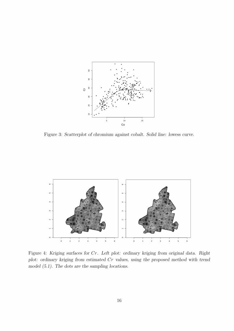
has already been reported by [26] and [13]. From an initial non-spatial descriptive analysis

(see Figure 3), we observe a clear nonlinear relationship between Cr and Co.

We apply the method proposed in this paper to model the relation between these two

metals, considering a sigmoidal curve:

Cr(s) =θ0

1 + exp(θ1 − θ2 · Co(s))+ ε(s). (5.1)

15

5 10 15

1020

3040

5060

Co

Cr

Figure 3: Scatterplot of chromium against cobalt. Solid line: lowess curve.

0 1 2 3 4 5 6

01

23

45

6

25

25

30

30

30

30

30

30

30

30

35

35

35

35

35

35

35 35

35

35

35

35

40 40 40

40

40

40

40

40

40

40

40

40

40

45

0 1 2 3 4 5 6

01

23

45

6

25

25

25

30

30

30

30

30

30

30

35

35

35

35

35

35

35

35

35

35 35

40

40

40

40

40

40

40

40

40

40

40

40

45

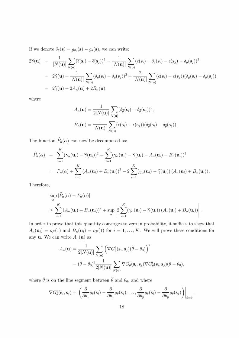
Figure 4: Kriging surfaces for Cr. Left plot: ordinary kriging from original data. Right

plot: ordinary kriging from estimated Cr values, using the proposed method with trend

model (5.1). The dots are the sampling locations.

16

The estimated parameters are θ0 = 41.74, θ1 = 1.47 and θ2 = 0.40. The first parameter

represents the asymptote, that is, the maximum value of Cr achieved, for growing concen-

trations of Co. θ1 provides information about the intercept and θ2 is the rate at which the

Cr concentration changes from its initial to its final value. We have assumed an exponential

model for the dependence structure, with estimated parameters φ = 0.10, σ2 = 62.92 and

nugget τ 2 = 13.11.

We have also obtained in Figure 4 kriging surfaces for the Cr and for the estimated values

of Cr, considering model (5.1). We can observe that the prediction surfaces are quite

similar, indicating that the large scale variation of the Cr is well described by its nonlinear

relationship with Co soil content.

6 Appendix

Proof of Proposition 3.1. For the sake of simplicity, we will restrict the proof to the

ordinary least squares estimator. The extension to a weighted least squares problem is

straightforward, taking into account assumption (A2). Note that αLS is the minimizer of

the function Pn(α) =∑K

i=1(γα(ui)− γ(ui))2. Define P (α) =

∑Ki=1(γα(ui)− γα0(ui))

2. We

prove the statement of the proposition by verifying the conditions of Theorem 5.7 in [23],

p. 45) for Mn = −Pn and M = −P , i.e. we will show that:

For all ε > 0, ∃ν > 0 : inf‖α−α0‖>ε

|P (α)− P (α0)| > ν (6.1)

∆n = supα∈A|Pn(α)− P (α)| P→ 0. (6.2)

Condition (6.1) follows from assumption (A3), since P (α0) = 0. By the proof of Theorem

3.1 in [17], we have that

∆0n = sup

α∈A|Pn(α)− P (α)| P→ 0,

where Pn(α) =∑K

i=1(γα(ui)− γ(ui))2 and 2γ(u) = |N(u)|−1

∑N(u)(ε(si)− ε(sj))2. We will

prove that:

supα∈A|Pn(α)− Pn(α)| P→ 0.

17

If we denote δθ(s) = gθ0(s)− gθ(s), we can write:

2γ(u) =1

|N(u)|∑

N(u)

(ε(si)− ε(sj))2 =1

|N(u)|∑

N(u)

(ε(si) + δeθ(si)− ε(sj)− δeθ(sj))2

= 2γ(u) +1

|N(u)|∑

N(u)

(δeθ(si)− δeθ(sj))2 +2

|N(u)|∑

N(u)

(ε(si)− ε(sj))(δeθ(si)− δeθ(sj))

= 2γ(u) + 2An(u) + 2Bn(u),

where

An(u) =1

2|N(u)|∑

N(u)

(δeθ(si)− δeθ(sj))2,

Bn(u) =1

|N(u)|∑

N(u)

(ε(si)− ε(sj))(δeθ(si)− δeθ(sj)).

The function Pn(α) can now be decomposed as:

Pn(α) =

K∑

i=1

(γα(ui)− γ(ui))2 =

K∑

i=1

(γα(ui)− γ(ui)− An(ui)− Bn(ui))2

= Pn(α) +

K∑

i=1

(An(ui) +Bn(ui))2 − 2

K∑

i=1

(γα(ui)− γ(ui)) (An(ui) +Bn(ui)) .

Therefore,

supα|Pn(α)− Pn(α)|

≤K∑

i=1

(An(ui) +Bn(ui))2 + sup

α

∣∣∣∣∣2K∑

i=1

(γα(ui)− γ(ui)) (An(ui) +Bn(ui))

∣∣∣∣∣ .

In order to prove that this quantity converges to zero in probability, it suffices to show that

An(ui) = oP (1) and Bn(ui) = oP (1) for i = 1, . . . , K. We will prove these conditions for

any u. We can write An(u) as

An(u) =1

2|N(u)|∑

N(u)

(∇Gt

θ(si, sj)(θ − θ0))2

= (θ − θ0)t1

2|N(u)|∑

N(u)

∇Gθ(si, sj)∇Gtθ(si, sj)(θ − θ0),

where θ is on the line segment between θ and θ0, and where

∇Gtθ(si, sj) =

(∂

∂θ1gθ(si)−

∂

∂θ1gθ(sj), . . . ,

∂

∂θpgθ(si)−

∂

∂θpgθ(sj)

)∣∣∣∣θ=θ

.

18

The convergence to zero in probability now follows from assumption (A4) and from the fact

that θP→ θ0 (see [11]). We can write Bn(u) as:

Bn(u) =1

|N(u)|∑

N(u)

(ε(si)− ε(sj))∇Gtθ(si, sj)(θ − θ0)

= (θ − θ0)t1

|N(u)|∑

N(u)

(ε(si)− ε(sj))∇Gθ(si, sj).

For simplicity, we assume that dim(Θ) = p = 1. When p > 1, it suffices to prove this

condition componentwise. Since θ converges in probability to θ0, we will prove that the

remaining part of Bn(u) is OP (1). Consider

∣∣∣ 1

|N(u)|∑

N(u)

(ε(si)− ε(sj))∇Gθ(si, sj)∣∣∣ ≤ c

|N(u)|∑

N(u)

|ε(si)− ε(sj)|,

where c := 2 supθ∈Θ,s∈D | ∂∂θgθ(s)| < ∞ by assumption (A4). Also, note that by assump-

tion (A1), the absolute differences |ε(si) − ε(sj)|, for (si, sj) ∈ N(u) follow a half-normal

distribution with variance 2γ(u)(1− 2/π). Hence, by Cauchy-Schwarz’s inequality,

Var

1

|N(u)|∑

N(u)

|ε(si)− ε(sj)|

≤ 1

|N(u)|2∑

(si,sj)∈N(u)

∑

(sk ,sl)∈N(u)

|Cov(|ε(si)− ε(sj)|, |ε(sk)− ε(sl)|)|

≤ 1

|N(u)|2∑

(si,sj)∈N(u)

∑

(sk ,sl)∈N(u)

√Var(|ε(si)− ε(sj)|)Var(|ε(sk)− ε(sl)|)

≤ 2γ(u)

(1− 2

π

)<∞.

It now easily follows that |N(u)|−1∑

N(u) |ε(si) − ε(sj)| = OP (1), using Tchebychev’s in-

equality. Hence, Bn(u) = oP (1). 2

Proof of Proposition 3.2. Similar to the proof of Proposition 3.1, we will check the

following conditions:

For all ε > 0, ∃ν > 0 : inf‖θ−θ0‖>ε

|Q(θ)−Q(θ0)| > ν (6.3)

Ωn = supθ∈Θ|Qn(θ)−Q(θ)| P→ 0, (6.4)

where

Q(θ) = 1 +R(θ) = 1 + limn→∞

1

nδtθΣ

−1δθ,

19

and δθ = (gθ0(s1)− gθ(s1), . . . , gθ0(sn) − gθ(sn))t. Condition (6.3) follows from assumption

(A5) and the fact that R(θ0) = 0. For (6.4) note that the function Qn(θ) can be decomposed

as:

Qn(θ) =1

n(Y − gθ)

t(L−1)tL−1(Y − gθ)

=1

n(ε+ δθ)

tΣ−1(ε+ δθ) = Qn1 +Qn2(θ) +Qn3(θ),

where

Qn1 =1

nεtΣ−1ε, Qn2(θ) =

2

nεtΣ−1δθ, Qn3(θ) =

1

nδtθΣ

−1δθ,

and ε = (ε1, . . . , εn)t. Then,

Ωn ≤ |Qn1 − 1|+ supθ∈Θ|Qn2(θ)|+ sup

θ∈Θ|Qn3(θ)− R(θ)|.

For notational convenience, write Σ = Σ(αLS) and Σ = Σ(α0). Note that

Qn1 =1

nεtΣ−1ε +

q∑

j=1

(αLSj − α0j)1

nεt∂Σ−1(α)

∂αjε,

for some α on the line segment between α0 and αLS. To show that the second term on

the right hand side is oP (1), first note that αLSj − α0j = oP (1) for all j = 1, . . . , q by

Proposition 3.1. Next, since α− α0 = oP (1), there exists a neighborhood N(α0) of α0 that

contains α with probability tending to one, and that is such that Σ(α) is positive definite

for all α ∈ N(α0). We will prove that(n−1εt ∂Σ−1(α)

∂αjε)

is OP (1) for j = 1, . . . , q. For that

purpose, note that ε is equal to Le, in distribution, for some et = (e1, . . . , en) ∼ Nn(0, In),

where In is the n× n identity matrix. Then:

1

n

∣∣∣etLt∂Σ−1(α)

∂αjLe∣∣∣

≤ 1

nsup

α∈N(α0)

∣∣∣etLt ∂Σ−1(α)

∂αjLe∣∣∣

≤ 1

nsup

α∈N(α0)

∣∣∣n∑

k=1

(Lt∂Σ−1(α)

∂αjL)kke2k

∣∣∣+2

nsup

α∈N(α0)

∣∣∣∑

k<l

(Lt∂Σ−1(α)

∂αjL)klekel

∣∣∣.

The first term on the right hand side is OP (1) by using similar arguments as for the term

Bn(u) in the proof of Proposition 3.1. For the second term, assumption (A1) entails that

the expression between absolute values is a degenerate U -process of order 2 indexed by

a Euclidean class of functions with square integrable envelope function. Hence, it follows

from Corollary 4 in [20] that the second term is also OP (1).

20

Now, consider1

nεtΣ−1ε =

1

n(L−1ε)t(L−1ε)

d=

1

n

n∑

i=1

e2i ,

where e1, . . . , en are i.i.d. N(0, 1) random variables. Hence n−1εtΣ−1εP→ 1. This shows

that Qn1− 1 = oP (1). We now turn to Qn2(θ). In a very similar way as for the term Bn(u)

in the proof of Proposition 3.1, we can show that supθ∈Θ |Qn2(θ)| = oP (1). Finally, for

Qn3(θ), it is readily seen that supθ∈Θ |Qn3(θ) − R(θ)| P→ 0, by using the weak consistency

of αLS established in Proposition 3.1. 2

Proof of Theorem 3.3. Consider Qn(θ) = Qn1 +Qn2(θ)+Qn3(θ), the same decomposition

as in the proof of Proposition 3.2. Since θ is defined as the minimizer of Qn(θ), we have

that ∇Qn(θ) = 0. If we examine the gradients of each addend in the decomposition of

Qn(θ), we see that ∇Qn1 = 0 and

∇Qn2(θ) =2

nG(θ)tΣ−1(αLS)ε, ∇Qn3(θ) = − 2

nG(θ)tΣ−1(αLS)δθ,

where ε and δθ are defined as in the proof of Proposition 3.2. The vector ∇Qn3(θ) can be

written after a first order Taylor expansion as

∇Qn3(θ) = − 2

nG(θ)tΣ−1(αLS)G(θ)(θ − θ0),

for some θ on the line segment between θ0 and θ. Therefore, for θ = θ we have the following

equality :

G(θ)tΣ−1(αLS)ε = G(θ)tΣ−1(αLS)G(θ)(θ − θ0).

It follows that

√n(θ − θ0) =

√n(G(θ)tΣ−1(αLS)G(θ)

)−1

G(θ)tΣ−1(αLS)ε.

Now, note that by Propositions 3.1 and 3.2, the estimators θ and αLS converge in probability

to θ0 and α0. Hence, by Slutsky’s theorem and noting that εd= Le with e ∼ Nn(0, In), it

follows that the previous variable converges in distribution to a normal random variable

with zero mean and covariance matrix S−1, where

S = limn→∞

1

nG(θ0)tΣ−1(α0)G(θ0),

which is well-defined by assumption (A6). 2

21

References

[1] Basu, S. and Reinsel, G.C. (1994) Regression models with spatially correlated errors.

Journal of the American Statistical Association, 89, 88-99.

[2] Besag, J. (1974) Spatial interaction and the statistical analysis of lattice systems.

Journal of the Royal Statistical Society, Series B, 36, 192-236.

[3] Chiles, J.P. and Delfiner, P. (1999) Geostatistics: Modeling Spatial Uncertainty. Wiley,

New York.

[4] Cressie, N. (1980) Robust estimation of the variogram. Journal of the International

Association for Mathematical Geology, 12, 115-125.

[5] Cressie, N. (1985) Fitting variogram models by weighted least squares. Journal of the

International Association for Mathematical Geology, 17, 563-586.

[6] Cressie, N.(1993) Statistics for Spatial Data. Wiley, New York.

[7] Desbarats, A.J., Logan, C.E., Hinton, M.J. and Sharpe, D.R. (2002) On the kriging

of water table elevations using collateral information from a digitial elevation model.

Journal of Hydrology, 255, 25-38.

[8] Diggle, P. and Ribeiro, P.J. (2007) Model-based Geostatistics. Springer, New York.

[9] Fazekas, I. and Klesov, O. (2000) A general approach to the strong law of large num-

bers. Theory of Probability and its Applications, 45, 569-583.

[10] Fuentes, M. (2005) A formal test for nonstationarity of spatial stochastic processes.

Journal of Multivariate Analysis, 96, 30-55.

[11] Gallant, A.R. and Goebel, J.J. (1976) Nonlinear regression with autocorrelated errors.

Journal of the American Statistical Association, 71, 961-967.

[12] Gambolati, G. and Galeati, G. (1987) Comments on Analysis of nonintrinsic spatial

variability by residual kriging with application to regional groundwater levels. Mathe-

matical Geology, 19, 249-257.

[13] Gerdol, R., Bragazza, L. and Marchesini, R. (2002) Element concentrations in the

forest moss Hylocomium splendens: variation associated with altitude, net primary

production and soil chemistry. Environmental Pollution, 116, 129-135.

[14] Goovaerts, P. (1997) Geostatistics for Natural Resources Characterization. Oxford Uni-

versity Press, New York.

22

[15] Haas, T. (1996) Multivariate spatial prediction in the presence of non-linear trend and

covariance non-stationarity. Environmetrics, 7, 145-165.

[16] Kim, H.J. and Boos, D.D. (2004) Variance estimation in spatial regression using non-

parametric semivariogram based on residuals. Scandinavian Journal of Statistics, 31,

387-401.

[17] Lahiri, S.N., Lee, Y. and Cressie, N. (2002) On asymptotic distribution and asymp-

totic efficiency of least squares estimators of spatial variogram parameters. Journal of

Statistical Planning and Inference, 103, 65-85.

[18] Matula, P. (1996) Convergence of weighted averages of associated random variables.

Probability and Mathematical Statistics, 16, 337-343.

[19] Ratkowsky, D.A. (1990) Handbook of Nonlinear Regression Models. Marcel Dekker,

New York.

[20] Sherman, R.P. (1994) Maximal inequalities for degenerate U-processes with applica-

tions to optimization estimators. Annals of Statistics, 22, 439-459.

[21] Snepvangers, J.J.J.C., Heuvelink, G.B.M. and Huisman, J.A. (2003) Soil water content

interpolation using spatio-temporal kriging with external drift. Geoderma, 112, 253-

271.

[22] Stein, M.A. (1999) Interpolation of Spatial Data. Springer, New York.

[23] Van der Vaart, A.W. (1998) Asymptotic Statistics. Cambridge University Press, Cam-

bridge.

[24] Verkatram, A. (1988) On the use of kriging in the spatial analysis of acid precipitation

data. Atmospheric Environment, 22, 1963-1975.

[25] White, H. and Domowitz, I. (1984) Nonlinear regression with dependent observations.

Econometrica, 52, 143-161.

[26] Zechmeister, H.G. (1995) Correlation between altitude and heavy metal deposition in

the Alps. Environmental Pollution, 89, 73-80.

23