ESE 531: Digital Signal Processing

Lec 18: March 26, 2018 Discrete Fourier Transform

Penn ESE 531 Spring 2018 – Khanna Adapted from M. Lustig, EECS Berkeley

Today

!  Adaptive filtering "  Blind equalization setup

!  Discrete Fourier Series !  Discrete Fourier Transform (DFT) !  DFT Properties !  Circular Convolution

2 Penn ESE 531 Spring 2018 - Khanna

Adaptive Filters

!  An adaptive filter is an adjustable filter that processes in time "  It adapts…

3

Adaptive Filter

Update Coefficients

x[n] y[n]

d[n]

e[n]=d[n]-y[n]

+ _

Penn ESE 531 Spring 2018 - Khanna

Adaptive Filter Applications

!  System Identification

4 Penn ESE 531 Spring 2018 - Khanna

Adaptive Filter Applications

!  Identification of inverse system

5 Penn ESE 531 Spring 2018 - Khanna

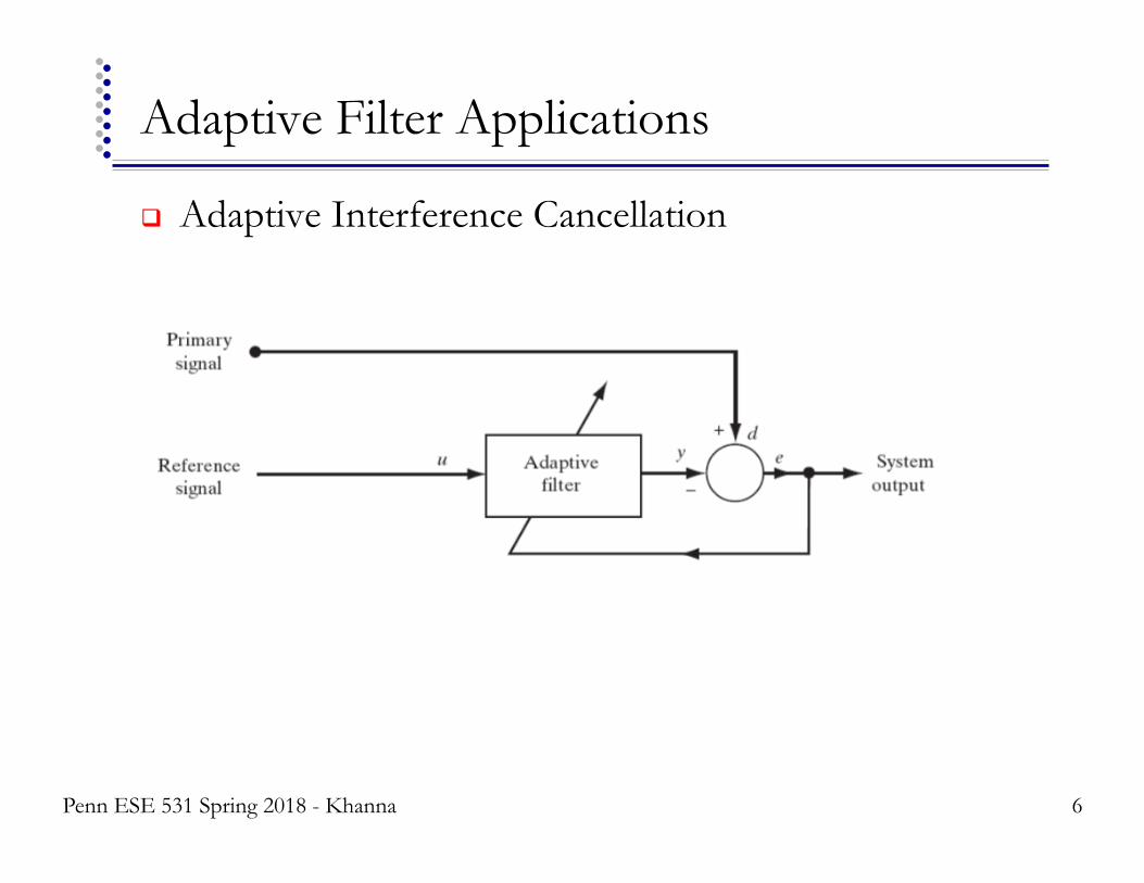
Adaptive Filter Applications

!  Adaptive Interference Cancellation

6 Penn ESE 531 Spring 2018 - Khanna

Adaptive Filter Applications

!  Adaptive Prediction

7 Penn ESE 531 Spring 2018 - Khanna

Discrete Fourier Series

Penn ESE 531 Spring 2018 - Khanna 8

Reminder: Eigenvalue (DTFT)

!  x[n]=ejωn

9 Penn ESE 531 Spring 2018 - Khanna

y[n]= x[n− k]h[k]k=−∞

∞

∑

= e jω (n−k )h[k]k=−∞

∞

∑

= e jωn h[k]k=−∞

∞

∑ e− jωk

= H (e jω )e jωn

H (e jω ) = h[k]k=−∞

∞

∑ e− jωk

!  Describes the change in amplitude and phase of signal at frequency ω

!  Frequency response !  Complex value

"  Re and Im "  Mag and Phase

Discrete Fourier Series

!  Definition: "  Consider N-periodic signal:

"  Frequency-domain also periodic in N:

"  “~” indicates periodic signal/spectrum

10 Penn ESE 531 Spring 2018 – Khanna Adapted from M. Lustig, EECS Berkeley

Discrete Fourier Series

!  Define:

!  DFS:

11 Penn ESE 531 Spring 2018 – Khanna Adapted from M. Lustig, EECS Berkeley

Discrete Fourier Series

!  Properties of WN:  "  WN

0 = WNN = WN

2N = ... = 1  "  WN

k+r = WNkWN

r and, WNk+N = WN

k 

!  Example: WNkn (N=6)

12 Penn ESE 531 Spring 2018 – Khanna Adapted from M. Lustig, EECS Berkeley

Discrete Fourier Transform

!  By convention, work with one period:

13

Same, but different!

Penn ESE 531 Spring 2018 – Khanna Adapted from M. Lustig, EECS Berkeley

Discrete Fourier Transform

!  The DFT

!  It is understood that,

14 Penn ESE 531 Spring 2018 – Khanna Adapted from M. Lustig, EECS Berkeley

DFS vs. DFT

15 Penn ESE 531 Spring 2018 – Khanna Adapted from M. Lustig, EECS Berkeley

Example

16 Penn ESE 531 Spring 2018 – Khanna Adapted from M. Lustig, EECS Berkeley

Example

17 Penn ESE 531 Spring 2018 – Khanna Adapted from M. Lustig, EECS Berkeley

Discrete Fourier Series

!  Properties of WN:  "  WN

0 = WNN = WN

2N = ... = 1  "  WN

k+r = WNkWN

r and, WNk+N = WN

k 

!  Example: WNkn (N=6)

18 Penn ESE 531 Spring 2018 – Khanna Adapted from M. Lustig, EECS Berkeley

Example

19 Penn ESE 531 Spring 2018 – Khanna Adapted from M. Lustig, EECS Berkeley

Example

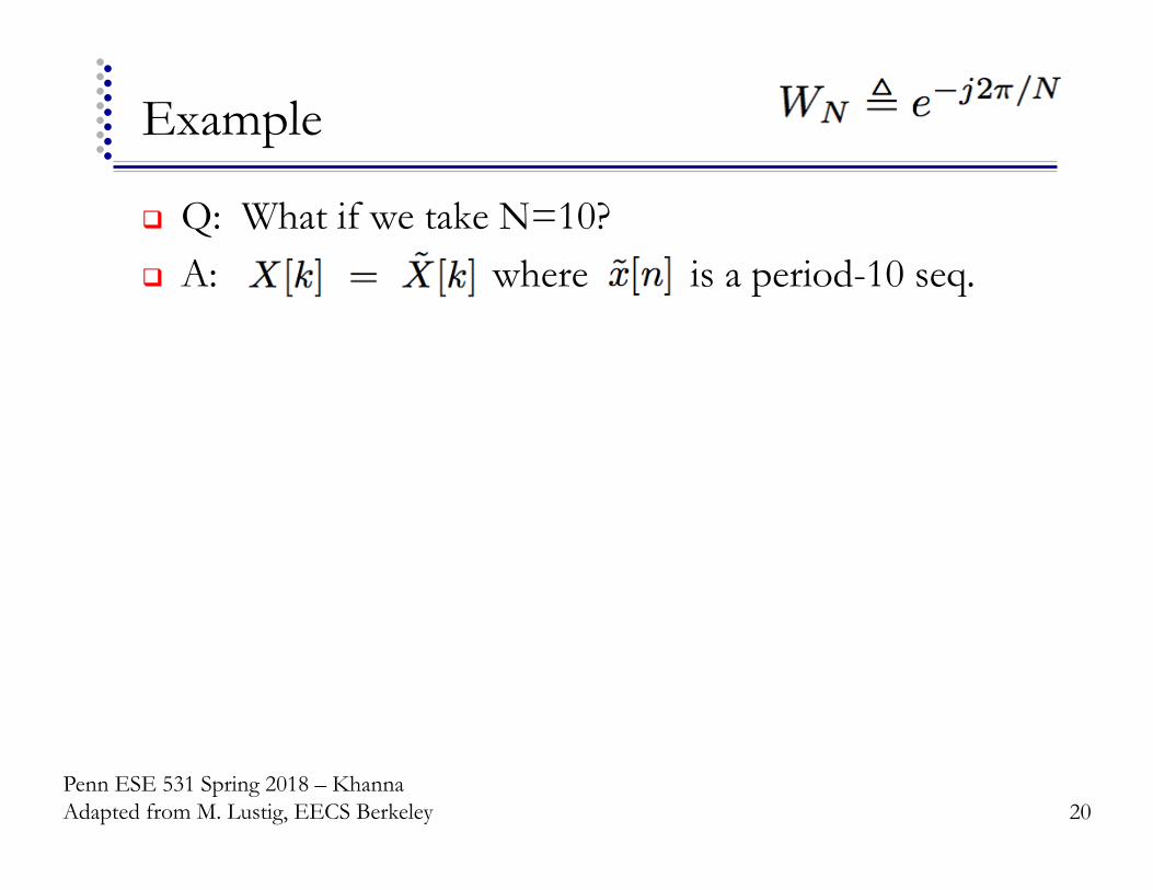
!  Q: What if we take N=10? !  A: where is a period-10 seq.

20 Penn ESE 531 Spring 2018 – Khanna Adapted from M. Lustig, EECS Berkeley

Example

!  Q: What if we take N=10? !  A: where is a period-10 seq.

21 Penn ESE 531 Spring 2018 – Khanna Adapted from M. Lustig, EECS Berkeley

Example

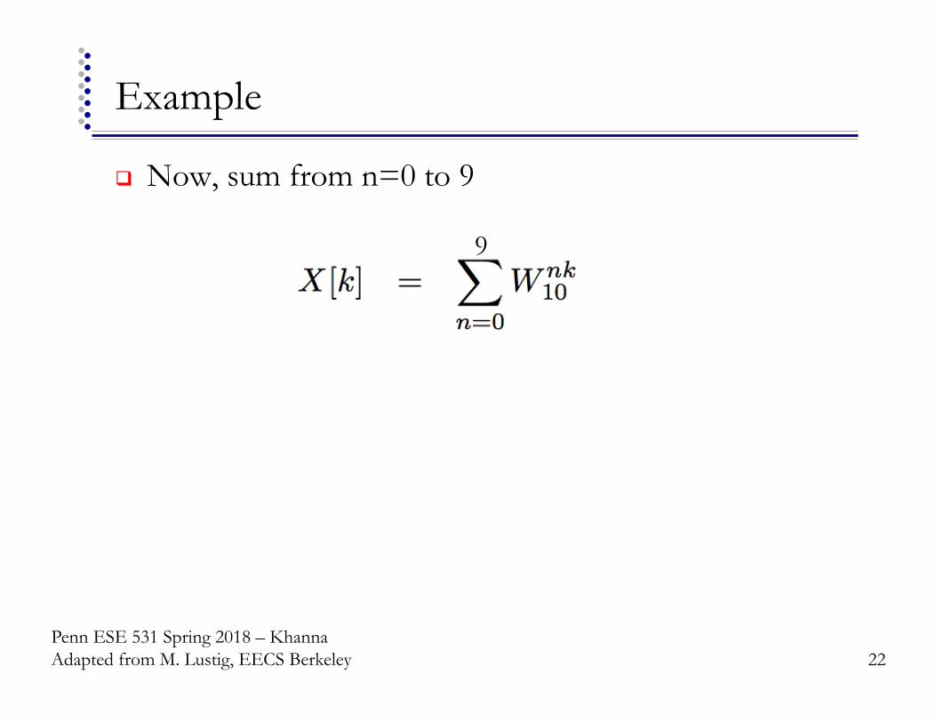
!  Now, sum from n=0 to 9

22

9

Penn ESE 531 Spring 2018 – Khanna Adapted from M. Lustig, EECS Berkeley

Example

!  Now, sum from n=0 to 9

23

9

4

Penn ESE 531 Spring 2018 – Khanna Adapted from M. Lustig, EECS Berkeley

DFT vs. DTFT

!  For finite sequences of length N: "  The N-point DFT of x[n] is:

"  The DTFT of x[n] is:

24 Penn ESE 531 Spring 2018 – Khanna Adapted from M. Lustig, EECS Berkeley

DFT vs. DTFT

!  The DFT are samples of the DTFT at N equally spaced frequencies

25 Penn ESE 531 Spring 2018 – Khanna Adapted from M. Lustig, EECS Berkeley

4

DFT vs DTFT

!  Back to example

26 Penn ESE 531 Spring 2018 – Khanna Adapted from M. Lustig, EECS Berkeley

4

DFT vs DTFT

!  Back to example

27 Penn ESE 531 Spring 2018 – Khanna Adapted from M. Lustig, EECS Berkeley

4

DFT vs DTFT

!  Back to example

28

Use fftshift to center around dc

Penn ESE 531 Spring 2018 – Khanna Adapted from M. Lustig, EECS Berkeley

DFT and Inverse DFT

!  Use the DFT to compute the inverse DFT. How?

29 Penn ESE 531 Spring 2018 – Khanna Adapted from M. Lustig, EECS Berkeley

DFT and Inverse DFT

!  Use the DFT to compute the inverse DFT. How?

30 Penn ESE 531 Spring 2018 – Khanna Adapted from M. Lustig, EECS Berkeley

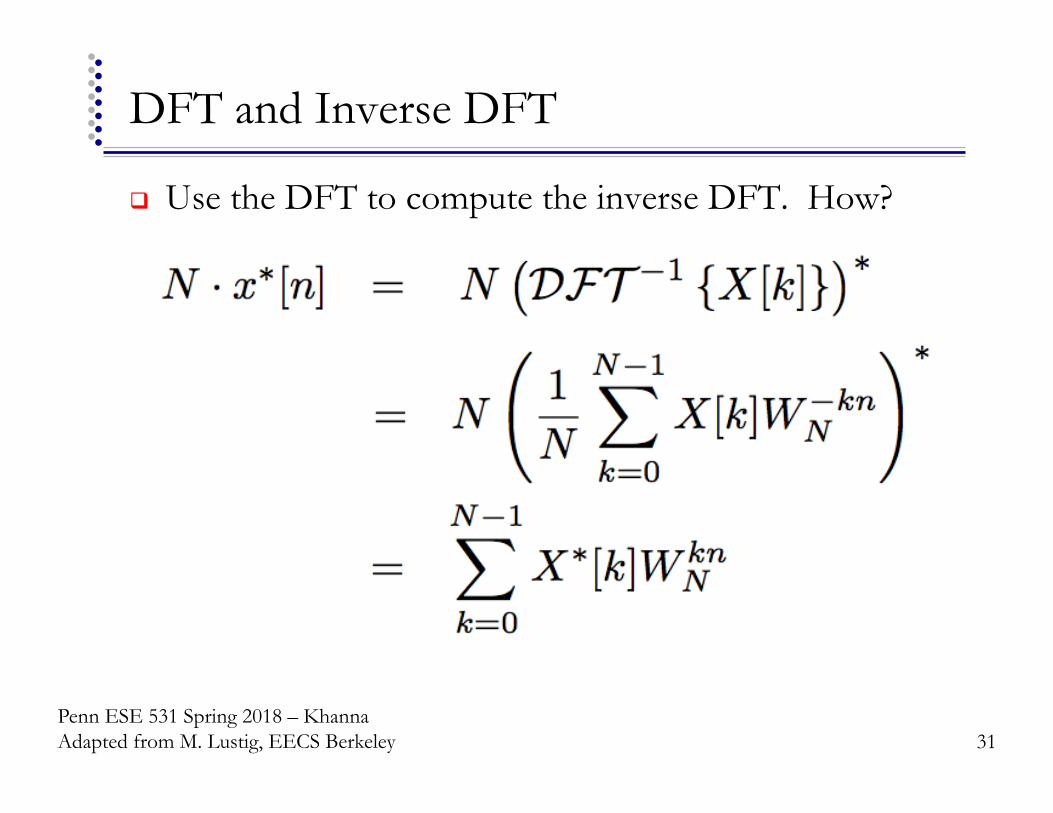
DFT and Inverse DFT

!  Use the DFT to compute the inverse DFT. How?

31 Penn ESE 531 Spring 2018 – Khanna Adapted from M. Lustig, EECS Berkeley

DFT and Inverse DFT

!  Use the DFT to compute the inverse DFT. How?

32 Penn ESE 531 Spring 2018 – Khanna Adapted from M. Lustig, EECS Berkeley

DFT and Inverse DFT

!  Use the DFT to compute the inverse DFT. How?

33 Penn ESE 531 Spring 2018 – Khanna Adapted from M. Lustig, EECS Berkeley

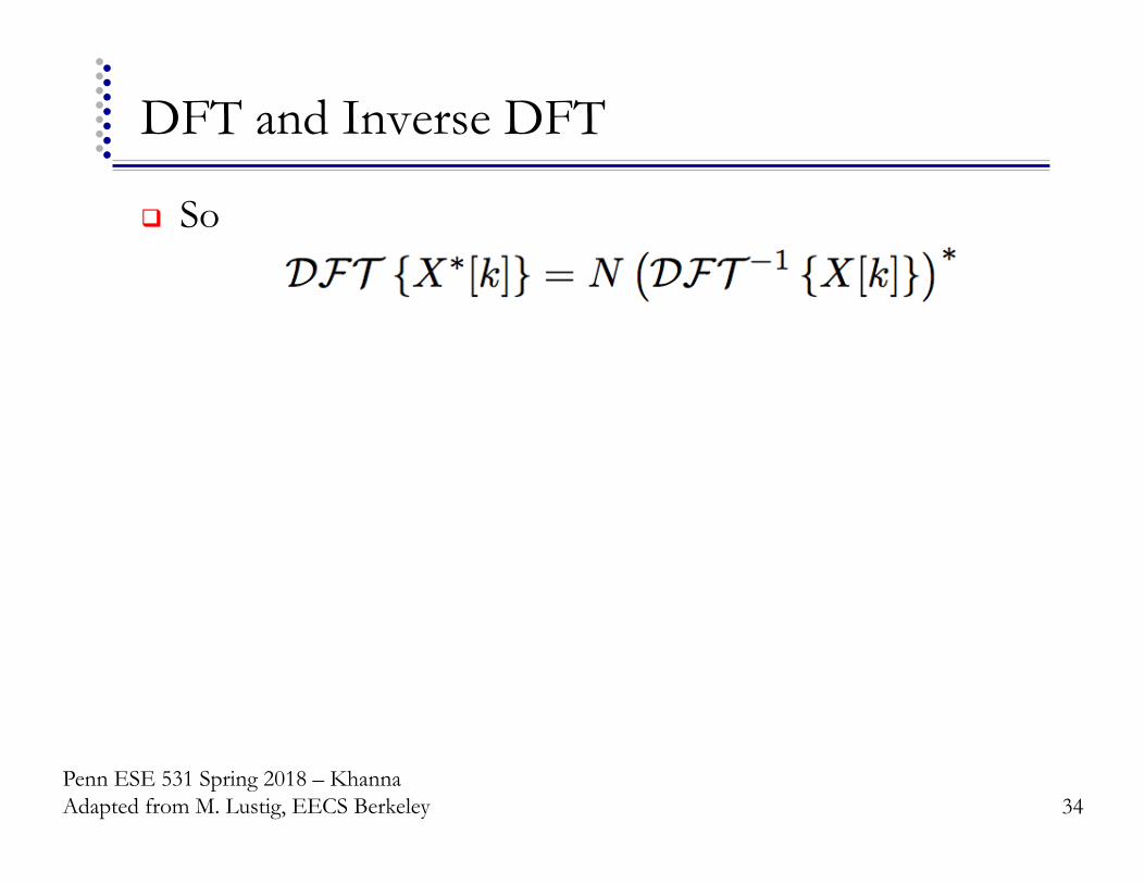
DFT and Inverse DFT

!  So

34 Penn ESE 531 Spring 2018 – Khanna Adapted from M. Lustig, EECS Berkeley

DFT and Inverse DFT

!  So

35 Penn ESE 531 Spring 2018 – Khanna Adapted from M. Lustig, EECS Berkeley

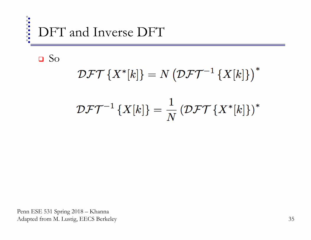
DFT and Inverse DFT

!  So

!  Implement IDFT by:

"  Take complex conjugate "  Take DFT "  Multiply by 1/N "  Take complex conjugate

36 Penn ESE 531 Spring 2018 – Khanna Adapted from M. Lustig, EECS Berkeley

DFT as Matrix Operator

37 Penn ESE 531 Spring 2018 – Khanna Adapted from M. Lustig, EECS Berkeley

DFT as Matrix Operator

38 Penn ESE 531 Spring 2018 – Khanna Adapted from M. Lustig, EECS Berkeley

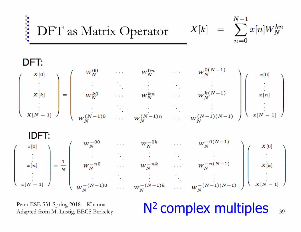
DFT as Matrix Operator

39 N2 complex multiples Penn ESE 531 Spring 2018 – Khanna Adapted from M. Lustig, EECS Berkeley

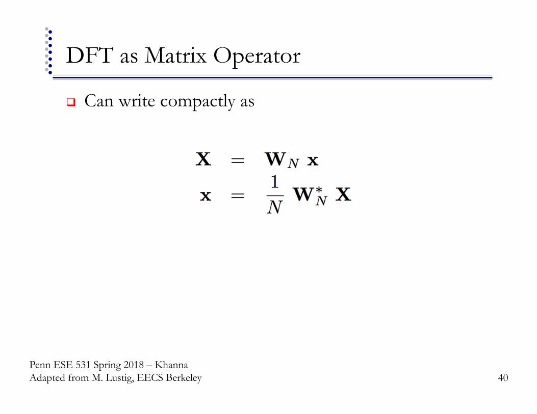
DFT as Matrix Operator

!  Can write compactly as

40 Penn ESE 531 Spring 2018 – Khanna Adapted from M. Lustig, EECS Berkeley

Properties of the DFT

!  Properties of DFT inherited from DFS !  Linearity

!  Circular Time Shift

41 Penn ESE 531 Spring 2018 – Khanna Adapted from M. Lustig, EECS Berkeley

Circular Shift

42 Penn ESE 531 Spring 2018 – Khanna Adapted from M. Lustig, EECS Berkeley

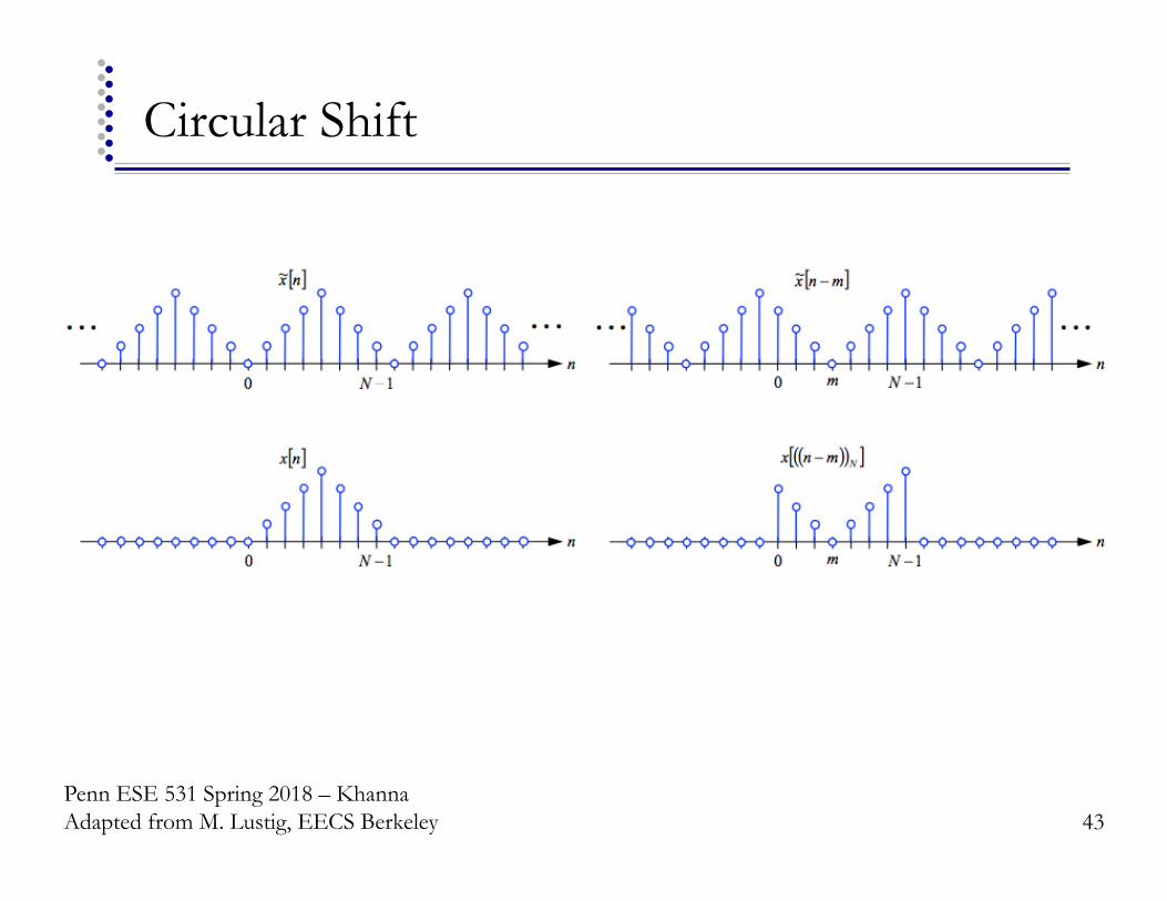
Circular Shift

43 Penn ESE 531 Spring 2018 – Khanna Adapted from M. Lustig, EECS Berkeley

Properties of DFT

!  Circular frequency shift

!  Complex Conjugation

!  Conjugate Symmetry for Real Signals

44 Penn ESE 531 Spring 2018 – Khanna Adapted from M. Lustig, EECS Berkeley

Example: Conjugate Symmetry

45 Penn ESE 531 Spring 2018 – Khanna Adapted from M. Lustig, EECS Berkeley

Example: Conjugate Symmetry

46 Penn ESE 531 Spring 2018 – Khanna Adapted from M. Lustig, EECS Berkeley

Example: Conjugate Symmetry

47 Penn ESE 531 Spring 2018 – Khanna Adapted from M. Lustig, EECS Berkeley

Example: Conjugate Symmetry

48 Penn ESE 531 Spring 2018 – Khanna Adapted from M. Lustig, EECS Berkeley

Example: Conjugate Symmetry

49 Penn ESE 531 Spring 2018 – Khanna Adapted from M. Lustig, EECS Berkeley

Example

50 Penn ESE 531 Spring 2018 – Khanna Adapted from M. Lustig, EECS Berkeley

Properties of the DFS/DFT

Penn ESE 531 Spring 2018 – Khanna Adapted from M. Lustig, EECS Berkeley

Properties (Continued)

Penn ESE 531 Spring 2018 – Khanna Adapted from M. Lustig, EECS Berkeley

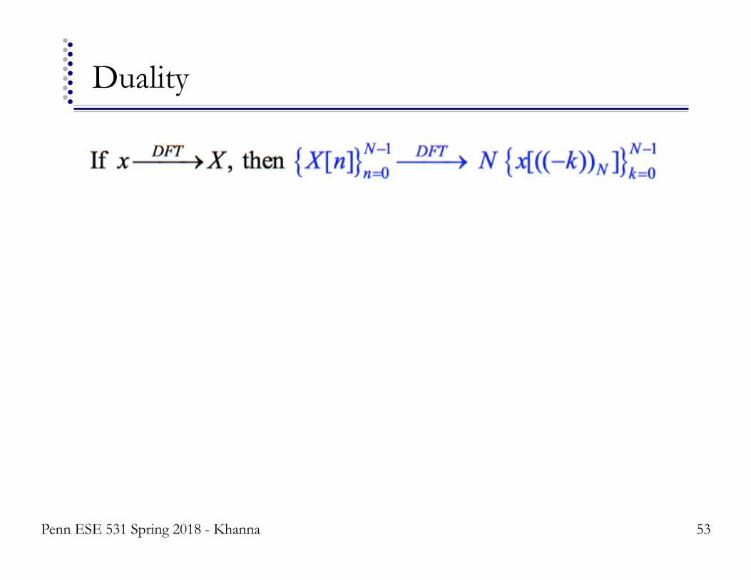
Duality

53 Penn ESE 531 Spring 2018 - Khanna

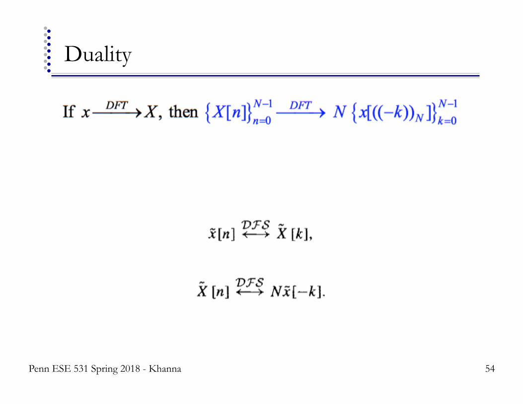
Duality

54 Penn ESE 531 Spring 2018 - Khanna

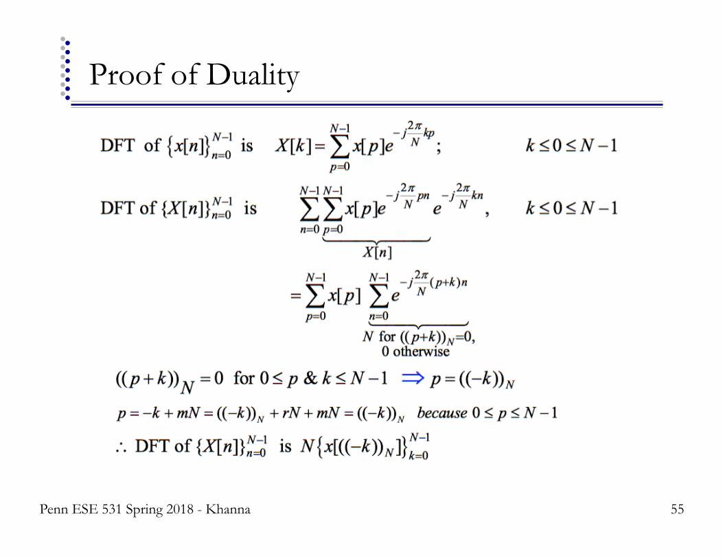
Proof of Duality

55 Penn ESE 531 Spring 2018 - Khanna

Circular Convolution

!  Circular Convolution:

For two signals of length N

56 Penn ESE 531 Spring 2018 – Khanna Adapted from M. Lustig, EECS Berkeley

Compute Circular Convolution Sum

57 Penn ESE 531 Spring 2018 – Khanna Adapted from M. Lustig, EECS Berkeley

Compute Circular Convolution Sum

58 Penn ESE 531 Spring 2018 – Khanna Adapted from M. Lustig, EECS Berkeley

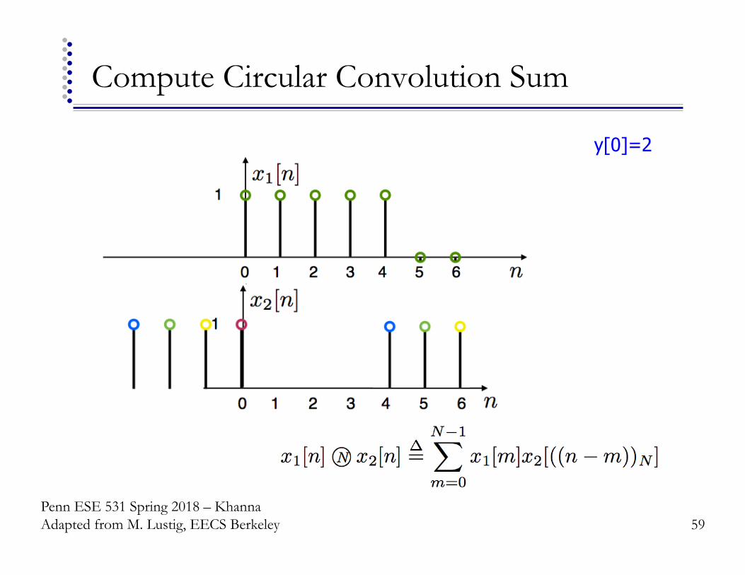
Compute Circular Convolution Sum

59

y[0]=2

Penn ESE 531 Spring 2018 – Khanna Adapted from M. Lustig, EECS Berkeley

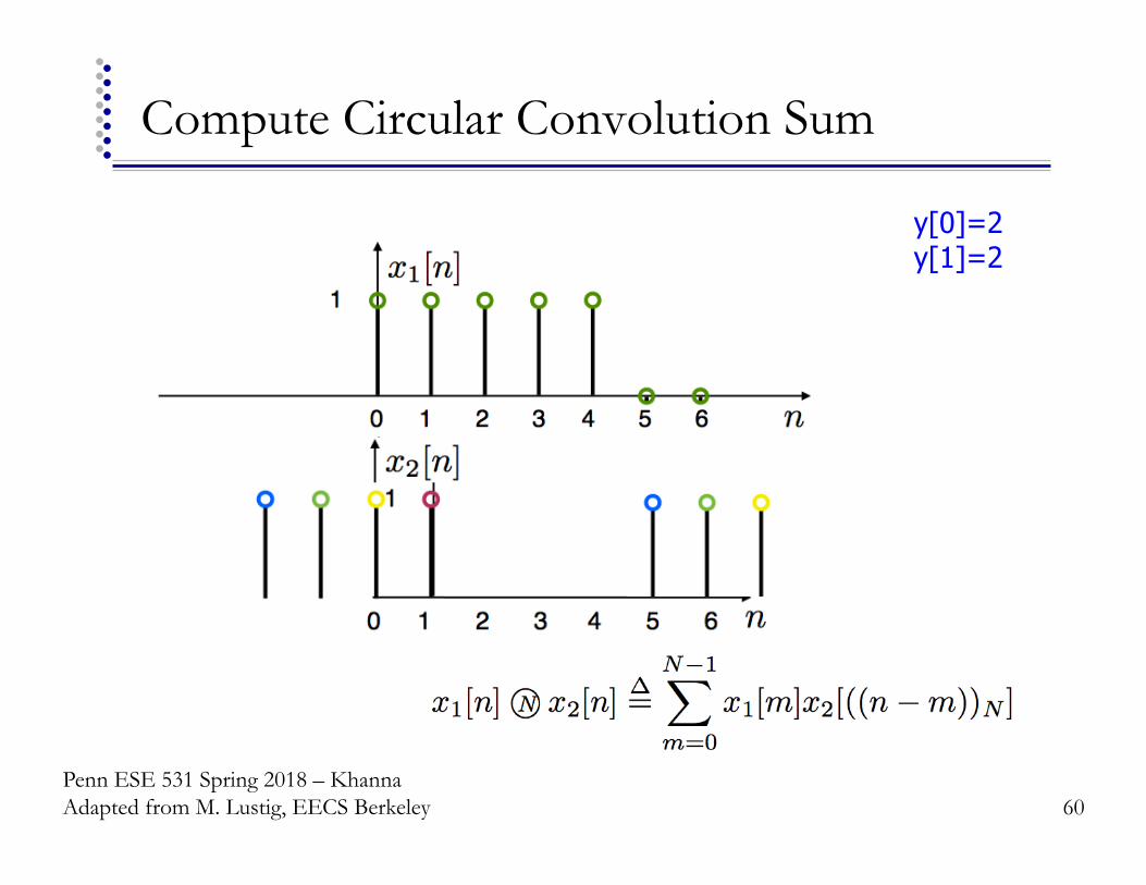
Compute Circular Convolution Sum

60

y[0]=2 y[1]=2

Penn ESE 531 Spring 2018 – Khanna Adapted from M. Lustig, EECS Berkeley

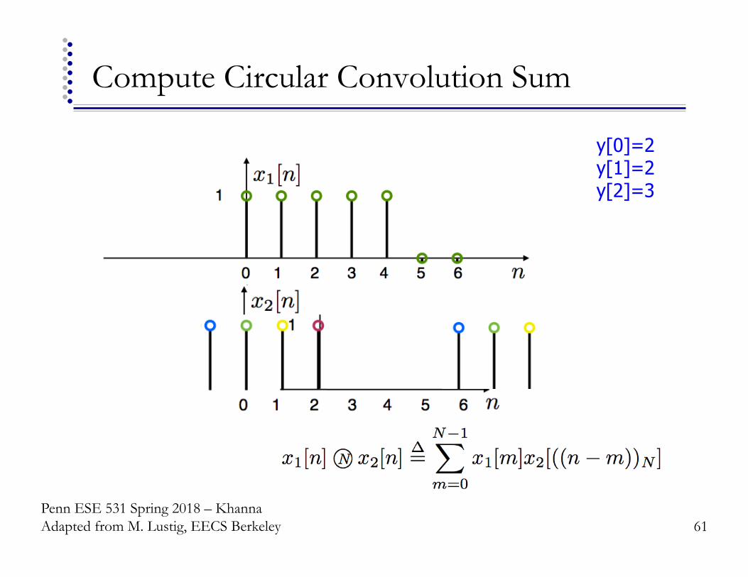
Compute Circular Convolution Sum

61

y[0]=2 y[1]=2 y[2]=3

Penn ESE 531 Spring 2018 – Khanna Adapted from M. Lustig, EECS Berkeley

Compute Circular Convolution Sum

62

y[0]=2 y[1]=2 y[2]=3 y[3]=4

Penn ESE 531 Spring 2018 – Khanna Adapted from M. Lustig, EECS Berkeley

Result

63

y[0]=2 y[1]=2 y[2]=3 y[3]=4

Penn ESE 531 Spring 2018 – Khanna Adapted from M. Lustig, EECS Berkeley

Circular Convolution

!  For x1[n] and x2[n] with length N

"  Very useful!! (for linear convolutions with DFT)

64 Penn ESE 531 Spring 2018 – Khanna Adapted from M. Lustig, EECS Berkeley

Multiplication

!  For x1[n] and x2[n] with length N

65 Penn ESE 531 Spring 2018 – Khanna Adapted from M. Lustig, EECS Berkeley

Linear Convolution

!  Next.... "  Using DFT, circular convolution is easy "  But, linear convolution is useful, not circular "  So, show how to perform linear convolution with circular

convolution "  Use DFT to do linear convolution

66 Penn ESE 531 Spring 2018 – Khanna Adapted from M. Lustig, EECS Berkeley

Big Ideas

!  Adaptive filtering "  Use LMS algorithm to update filter coefficients for

applications like system ID, channel equalization, and signal prediction

!  Discrete Fourier Transform (DFT) "  For finite signals assumed to be zero outside of defined

length "  N-point DFT is sampled DTFT at N points "  Useful properties allow easier linear convolution

!  DFT Properties "  Inherited from DFS, but circular operations!

67 Penn ESE 531 Spring 2018 – Khanna Adapted from M. Lustig, EECS Berkeley

Admin

!  HW 7 out now "  Due Friday

!  Project posted Friday "  Work in groups of up to 2

"  Can work alone if you want "  Use Piazza to find partners

68 Penn ESE 531 Spring 2018 – Khanna Adapted from M. Lustig, EECS Berkeley