Conjugate directions○

Conjugate Gram-Schmidt○

The conjugate gradient (CG) algorithm○

Solving linear systems○

Leontief input-output model of an economy○

Conjugate direction methods•This lecture:

Instructor: Amir Ali Ahmadi

Fall 2014

In the last couple of lectures we have seen several types of gradient descent methods as well as the Newton's method. Today we see yet another class of descent methods that are particularly clever and efficient: the conjugate direction methods.

•

This method is primarily developed for minimizing quadratic functions. A classic reference is due to Hestenes and Stiefel [HS52], but some of the ideas date back further.

•

They minimize a quadratic function in variables in steps (in absence of roundoff errors).

○

Evaluation and storage of the Hessian matrix is not required.○

Unlike Newton, we do not need to invert a matrix (or solve a linear system) as a sub-problem.

○

Conjugate direction methods are in some sense intermediate between gradient descent and Newton. They try to accelerate the convergence rate of steepest descent without paying the overhead of Newton's method. They have some very attractive properties:

•

Conjugate direction methods are also used in practice for solving large-scale linear systems; in particular those defined by a positive definite matrix.

•

Like our other descent methods, conjugate direction methods take the following iterative form:

•

The direction is chosen using the notion of conjugate directions which is fundamental to everything that follows. So let us start with defining that formally.

•

Our presentation in this lecture is mostly based on [CZ13] but also adapts ideas from [Ber03], [Boy13], [HS52], [Kel09], [Lay03], [She94].

•

TAs: Y. Chen, G. Hall, J. Ye

Lec10p1, ORF363/COS323

Lec10 Page 1

Definition. Let be an real symmetric matrix. We say that a set of non-zero vectors are -conjugate if

In this lecture we are mostly concerned with minimizing a quadratic function

where

If is the identity matrix, this simply means that the vectos are pairwise orthogonal.

•

For general [She94] gives a nice intution of what -conjugacy means. Figure (a) below shows the level sets of a quadratic function and a number of -conjugate pairs of vectors. "Imagine if this page was printed on bubble gum, and you grabbed Figure (a) by the ends and stretched in until the ellipse appear circular. Then vectors would appear orthogonal, as in Figure (b)."

•

The pairs on the left are -conjugate because the pairs on the right are orthogonal.

Image: [She94]

Recall that a set of vectors are linearly independent if for any sets of scalars we have

•

Lec10p2, ORF363/COS323

Lec10 Page 2

Lemma 1. Let be an symmetric positive definite matrix. If the directions are -conjugate, then they are linearly independent.

Proof.

Remark. Why in the statement of the lemma we have Because we cannot have more than linearly independent vectors in (basic fact in linear algebra, proven for your convenience below). Hence we cannot have more than vectors that are -conjugate.

Lec10p3, ORF363/COS323

Lec10 Page 3

So what are -conjugate directions good for? As we will see next, if we have

conjugate directions, we can minimize

by doing

exact line search iteratively along them. This is the conjugate direction method. Let's see it more formally.

Input: An matrix A set of -conjugate directions

The Conjugate Direction Algorithm: Pick an initial point For to

Let •

Let

•

Let •

Lemma 2. The step size given above gives the exact minimum along the direction

And more importantly,

Theorem 1. For any starting point the algorithm above converges to

the unique minimum of

in steps; i.e.,

Proof of Lemma 2.

Lec10p4, ORF363/COS323

Lec10 Page 4

Proof of Theorem 1.

Lec10p5, ORF363/COS323

Lec10 Page 5

The algorithm we presented assumed a list of -conjugate directions as input. But how can compute these directions from the matrix ? Here we propose a simple algorithm (and we'll see a more clever approach later in the lecture).

The conjugate Gram-Schmidt procedure

This is a simple procedure that allows us to start with any set of linearly independent vectors (say, the standard basis vectors ) and turn them into -conjugate vectors in such a way that and span the same subspace. In the special case that is the identity matrix, this is the usual Gram-Schmidt process for obtaining an orthogonal basis.

Jorgen Gram(1850-1916)

Erhard Schmidt(1876-1959)

Theorem 2. Let be an positive definite matrix and let be a set of linearly independent vectors. Then, the vectors constructed as follows are -conjugate (and span the same space as ) :

Proof.

Lec10p6, ORF363/COS323

Lec10 Page 6

Proof (Cont'd).

While you can always use the conjugate Gram-Schmidt algorithm to generate conjugate directions and then start your conjugate direction method, there is a much more efficient way of doing this.

•

This method can generate your conjugate directions on the fly in each iteration.

○

Moreover, The update rule to find new conjugate directions will be more efficient that what the Gram-Schmidt process offered, which requires a stack of all previous conjugate directions in the memory.

○

This is the conjugate gradient (CG) algorithm that we will see shortly. •

Before we get to the conjugate gradient algorithm, we state an important geometric property of any conjugate direction method called the "expanding subspace theorem". The proof of this comes up in the proof of correctness of the conjugate gradient algorithm.

•

Lec10p7, ORF363/COS323

Lec10 Page 7

Theorem 3 (the expanding subspace theorem). Let be an

symmetric positive definite matrix,

a set

of -conjugate directions, an arbitrary point in , and the sequence of points generated by the conjugate direction algorithm. Let

Then, for minimizes over

Lemma 3. Let be an symmetric positive definite matrix,

a set of -conjugate directions, an arbitrary

point in , and the sequence of points generated by the conjugate direction algorithm. Let Then,

for all and

Image credit: [CZ13]

Note that So this proves again that the algorithm indeed terminates with the optimal solution in steps.

•Remark:

The following lemma is the main ingredient of the proof.

Lec10p8, ORF363/COS323

Lec10 Page 8

Proof of Lemma 3.

Proof of the expanding subspace theorem.

Lec10p9, ORF363/COS323

Lec10 Page 9

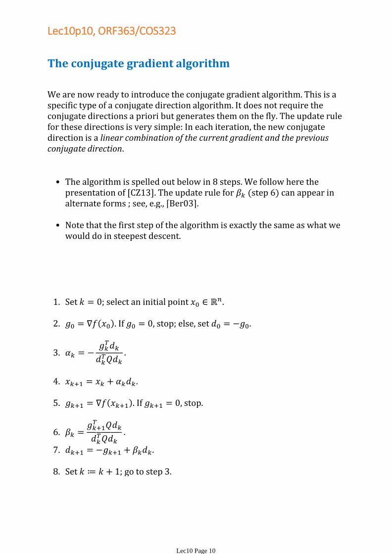
The conjugate gradient algorithm

We are now ready to introduce the conjugate gradient algorithm. This is a specific type of a conjugate direction algorithm. It does not require the conjugate directions a priori but generates them on the fly. The update rule for these directions is very simple: In each iteration, the new conjugate direction is a linear combination of the current gradient and the previous conjugate direction.

Set select an initial point 1.

If , stop; else, set 2.

3.

4.

If stop.5.

6.

7.

Set go to step 3.8.

The algorithm is spelled out below in 8 steps. We follow here the presentation of [CZ13]. The update rule for (step 6) can appear in alternate forms ; see, e.g., [Ber03].

•

Note that the first step of the algorithm is exactly the same as what we would do in steepest descent.

•

Lec10p10, ORF363/COS323

Lec10 Page 10

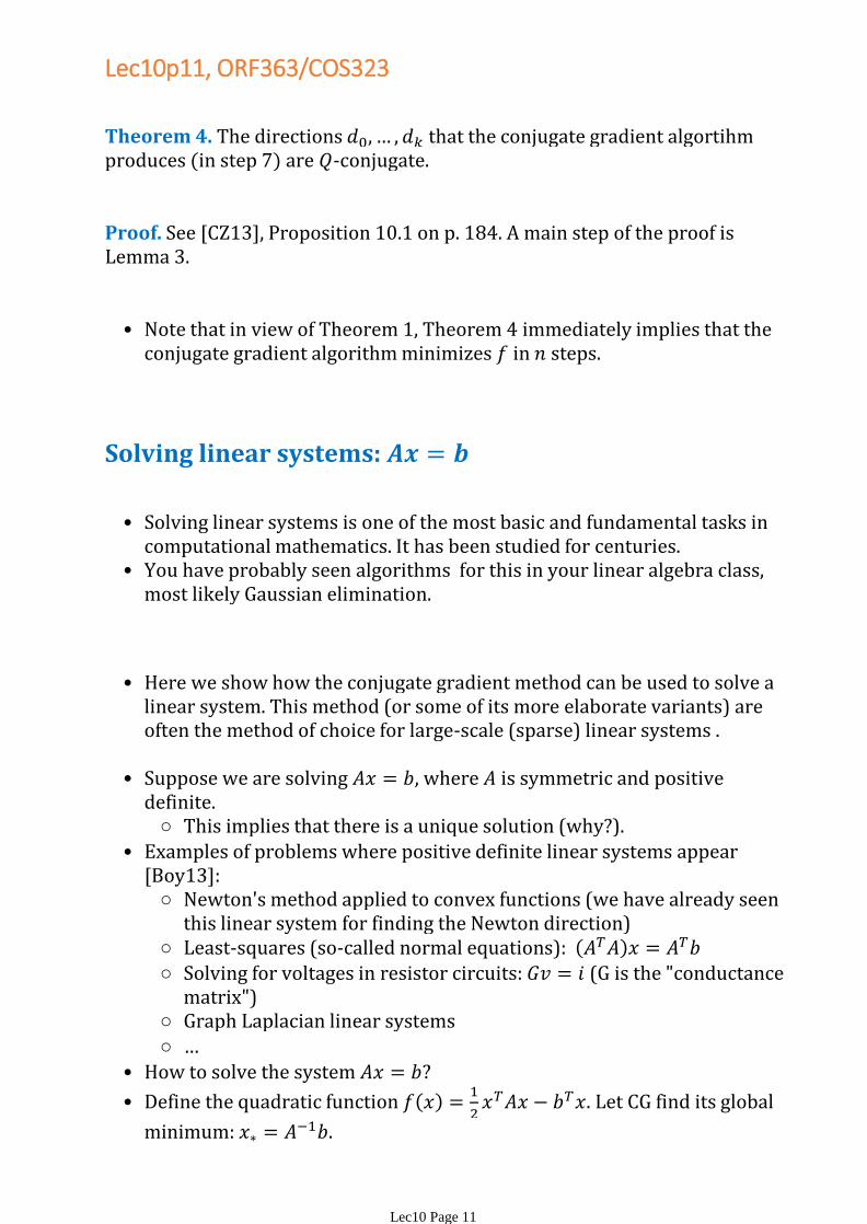
Theorem 4. The directions that the conjugate gradient algortihm produces (in step 7) are -conjugate.

Proof. See [CZ13], Proposition 10.1 on p. 184. A main step of the proof is Lemma 3.

Note that in view of Theorem 1, Theorem 4 immediately implies that the conjugate gradient algorithm minimizes in steps.

•

Solving linear systems:

Solving linear systems is one of the most basic and fundamental tasks in computational mathematics. It has been studied for centuries.

•

You have probably seen algorithms for this in your linear algebra class, most likely Gaussian elimination.

•

Here we show how the conjugate gradient method can be used to solve a linear system. This method (or some of its more elaborate variants) are often the method of choice for large-scale (sparse) linear systems .

•

This implies that there is a unique solution (why?).○

Suppose we are solving where is symmetric and positive definite.

•

Newton's method applied to convex functions (we have already seen this linear system for finding the Newton direction)

○

Least-squares (so-called normal equations): ○

Solving for voltages in resistor circuits: (G is the "conductance matrix")

○

Graph Laplacian linear systems○

…○

Examples of problems where positive definite linear systems appear [Boy13]:

•

How to solve the system •

Define the quadratic function

Let CG find its global

minimum:

•

Lec10p11, ORF363/COS323

Lec10 Page 11

Is the assumption too restrictive?•

Suppose we want to solve , where is invertible but not positive definite or even symmetric.

○

Claim: if and only if ○

Note that is symmetric. It is also positive definite if is invertible (why?).

○

So we can solve using CG instead.○

No (at least not in theory). Indeed, any nondegenerate linear system can be reduced to a positive definite one:

•

For example, the condition number of the second linear system is the square of that of the first one. (Why? Recall that condition

number is

)

○

Moreover, we don't want to pay the price of matrix multiplication to get The good news is that we don't have to: In the CG algorithm only matrix-vector operations are needed and we can do them from right to left by two matix-vector multiplications instead of first doing the matrix-matrix multiplicaiton.

○

But there is a word of caution: while this simple reduction is mathematically valid, it may raise concerns from a numerical point of view.

•

Leontief input-output model of an economy

(1973)

Wassily Leontief(1906-1999)

Agriculture○

Manufacturing ○

Services○

Education○

…○

The Leontief input-output model breaks a nation's economy into sectors (so-called producing sectors). For example,

•

Separately, it considers the society as an "open sector" which is a consumer of the output of the sectors.

•

Each of the sectors also needs the output of (some of) the other sectors in order to produce its own output.

•

The model tries to understand the interdependencies among the sectors by studying how much each sector should produce to meet the demand of the other sectors, as well as the demand of the society.

•

Lec10p12, ORF363/COS323

Lec10 Page 12

Leontief input-output model (Cont'd)

Transportation Agriculture Services Manufacturing

Transportation .2 .3 .5 .3

Agriculture .5 .3 .1 .0

Services .1 .2 .2 .5

Manufacturing .1 .1 .1 .1

This is called the consumption matrix, denoted by •

In order to produce one unit of transportation, the transportation industry needs to consume as input .2 units of transportation itself, .5 units of agriculture, .1 unites of services, and .1 units of manufacturing.

○

Other columns interpreted analogously. ○

Here is how you should interpret the first column:•

Input consumed per unit of output

Let be an vector denoting the demand of the open sector (i.e., the society or the non-producing sector) for each of the producing sectors.

•

We are interested in solving the following linear system, which is called the Leontief production equation:

•

Here, is the amount that sector needs to produce to meet intermidate demand (demand of other producing sectors) and the final demand (demand of the open sector).

•

"Amount produced = intermediate demand + final demand"

So for a given and we need to solve the following liner system to figure out how much each sector should produce:

•

A sufficient condition for this is for to have spectral radius (i.e., largest eigenvalue in absolute value) less than one. Can you prove this?

○

An economy is called "productive" if for every demand vector there exists a nonnegative production vector satisfying the above linear system. This is a property of the consumption matrix only.

•

Lec10p13, ORF363/COS323

Lec10 Page 13

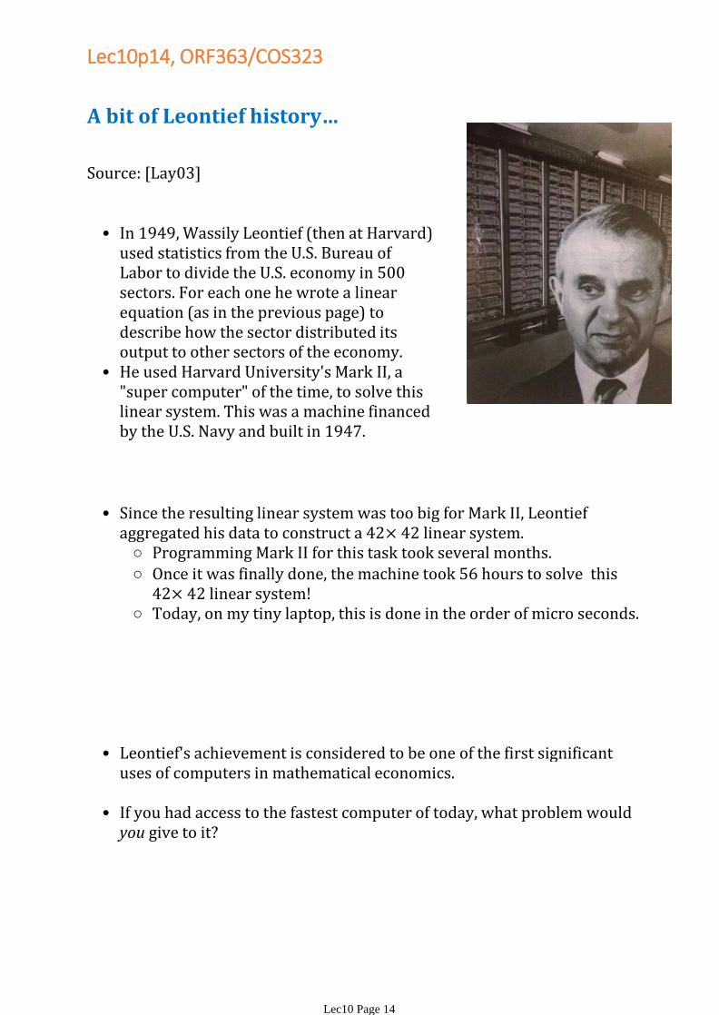
A bit of Leontief history…

Source: [Lay03]

In 1949, Wassily Leontief (then at Harvard) used statistics from the U.S. Bureau of Labor to divide the U.S. economy in 500 sectors. For each one he wrote a linear equation (as in the previous page) to describe how the sector distributed its output to other sectors of the economy.

•

He used Harvard University's Mark II, a "super computer" of the time, to solve this linear system. This was a machine financed by the U.S. Navy and built in 1947.

•

Programming Mark II for this task took several months.○

Once it was finally done, the machine took 56 hours to solve this 42 linear system!

○

Today, on my tiny laptop, this is done in the order of micro seconds.○

Since the resulting linear system was too big for Mark II, Leontief aggregated his data to construct a 42 linear system.

•

Leontief's achievement is considered to be one of the first significant uses of computers in mathematical economics.

•

If you had access to the fastest computer of today, what problem would you give to it?

•

Lec10p14, ORF363/COS323

Lec10 Page 14

References:

[Ber03] D.P. Bertsekas. Nonlinear Programming.Second edition. Athena Scientific, 2003.

-

[Boy13] S. Boyd. Lecture slides for Convex Optimization II. Stanford University, 2013. http://stanford.edu/class/ee364b/

-

[CZ13] E.K.P. Chong and S.H. Zak. An Introduction to Optimization. Fourth edition. Wiley, 2013.

-

[HS52] M. R. Hestenes and E. Stiefel. Methods of conjugate gradients for solving linear systems. Journal of Research of the National Bureau of Standards, Vol. 49, No. 6, 1952.

-

[Kel09] J. Kelner. Topics in theoretical computer science: an algorithmist's toolkit, MIT OpenCourseWare, 2009.

-

[Lay03] D. C. Lay. Linear Algebra and its Applications. Third edition. Addison Wesley, 2003.

-

[She94] J.R. Shewchuk. "An introduction to the conjugate gradient method without the agonizing pain", (1994).

-

Notes:The relevant [CZ13]chapter for this lecture is Chapter 10.

Lec10p15, ORF363/COS323

Lec10 Page 15