lec12: shape models and medical image segmentation

MEDICAL IMAGE COMPUTING (CAP 5937)

LECTURE 12: Shape Models and Medical Image Segmentation

Dr. Ulas BagciHEC 221, Center for Research in Computer Vision (CRCV), University of Central Florida (UCF), Orlando, FL [email protected] or [email protected]

1SPRING 2017

Outline• Shape Information

– Representation– Simple processing (dilation + erosion)

• Shape Modeling– M-reps– Active Shape Models (ASM)– Oriented Active Shape Models (OASM)– Application in anatomy recognition and segmentation– Comparison of ASM and OASM

2

3MotivationMost structures of clinical interest have a characteristic shape and anatomical location relative to other structures

Brain image shows: • Ventricles • Caudate nucleus • Lentiform nucleus

4Motivation

Heart model with large vessels

What is Shape?

5

What is Shape?• Shape is any connected set of points!

6

What is Shape?• Shape is any connected set of points!

7

Shape (S) Points

T: boundaryP: interiorQ: exterior

Example Applications for Shape Analysis

8

NeuroScience

• Morphological taxonomy of neural cells

• Interplay between form and function

• comparisons between cells of different cortical areas

• Comparisons between cells of different species

• …

Internet/Document Analysis

• Content-based information retrieval

• Watermarking• Graphic design• WWW• Optical character

recognition• Multimedia databases• …

Visual Arts

• Video restoration• Video tracking• Special effects• Games• Computer graphics• Image synthesis• Visualizations• …

Imaging/Vision

• Pathology detection/classification (spiculated and spherical nodules)

• 3D pose estimation• Morphological

operations• Anatomy modeling• Segmentation• Registration• Volumetry

Other areas: medicine, biology, engineering, physics, agriculture, security…

Shape Models• Point distribution, Active Shape, Active Appearance

models (Cootes & Taylor)• Fourier Snakes (Szekely)• Active Contours (Blake)• Parametrically-deformable models (Staib & Duncan)• Medial Representation (m-rep)• …

9

Shape Models• Point distribution, Active Shape, Active Appearance

models (Cootes & Taylor)• Fourier Snakes (Szekely)• Active Contours (Blake)• Parametrically-deformable models (Staib & Duncan)• Medial Representation (m-rep)• …

10

Active Shape Models can be used to help interpret new images by finding the parameters which best match an

instance of the model to the image.

The shape of an organ can be characterized as being a transformed version of some template

11

template

Credit: Parmedco.ir

Deformations/transformation

What shape representation is for• Analysis from images– Extract the kidney-shaped object

– Register based on the pelvic bone shapesCredit: Pizer

What shape representation is for

13

Snapshots of subcortical shapeevolution after geodesicregression on a multi-object

complex: putamen, amygdala, and hippocampus.

Credit: Gerig


14

A graphical visualization is presented forthe left/right asymmetry of the amygdala–hippocampal complex for healthy controls (top row) and patients with schizophrenia (bottom row).


• Shape science – Shape and biology– Shape-based diagnosis

Brain structures (Gerig)

Primitives for shape representation: Landmarks

• Sets of points of special geometry

Primitives for shape representation: Boundaries

• Boundary points with normals

Medial Primitives

Representing Boundary Displacements

• Along figurally implied boundary normals• Coarse-to-fine• Captures along-boundary covariance

• Useful for rendering

Medial Primitives• x, (b,n) frame, r, θ (object angle)• Imply boundary segments

with tolerance

• Similarity transform equi-variant– Zoom invariance implies width-proportionality of

• tolerance of implied boundary• boundary curvature distribution• spacing along net• interrogation aperture for image

θ

b

rR(- θ)b x rR(θ)bn

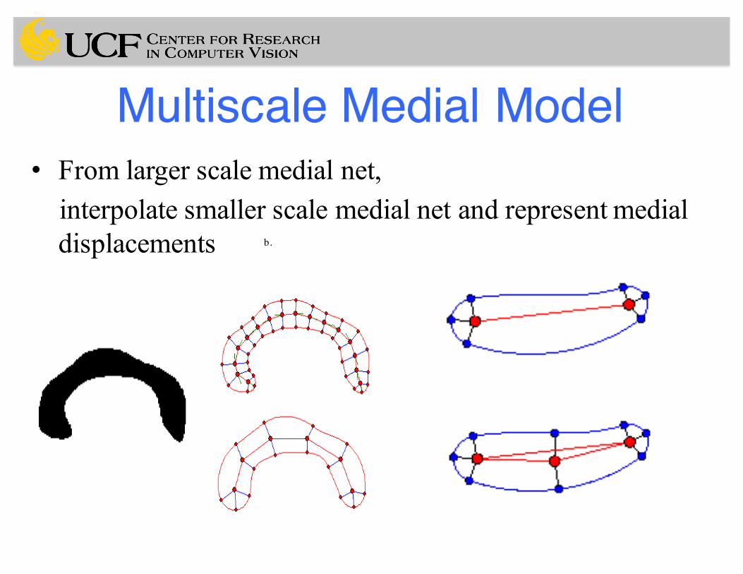
Multiscale Medial Model• From larger scale medial net,

interpolate smaller scale medial net and represent medial displacements b.

Medial Net Shape Models

Medial nets, positions onlyMedial net

Active Shape Model (T. Cootes et al., 1995)

• Representation of Shapes– Point Distribution Model (PDM)– Represent a shape instance by a judiciously chosen set of points

(features), each of which is a k-dim vector. N feature points are stacked into a long vector of length kn:

where

23

q = [p1, . . . , pn]T

pi = (xi, yi), for i = 1, ..., n

landmarks

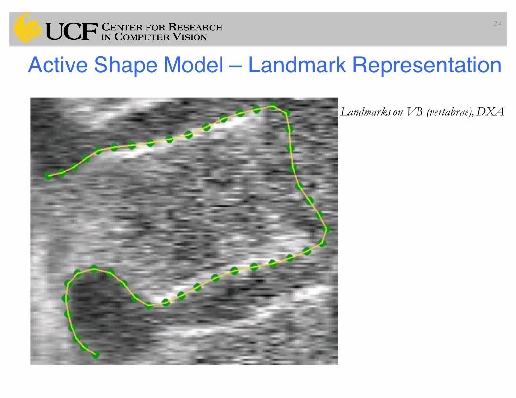
Active Shape Model – Landmark Representation

24

Landmarks on VB (vertabrae), DXA

Active Shape Model – How to?(1) Build a statistical boundary shape model that consists of a mean

shape and its allowable variations.

(2) Use the model to recognize the boundary in the given scene.

(3) Use the model to fit to the information in the scene. The resulting model is considered to be the boundary delineation.

25

(1) Mean Shape• Model is constructed via a set of landmarks or homologous points.

• Align the shapes after landmarking corresponding points– The Procrustes Algorithm is used to that the sum of instances to the

mean of each shape is minimized! Why?

• The mean shape and allowable variations are determined from a set of N training shapes

26

X

i=1,...,M

(qi � q̄)2

(1) Mean Shape

27

……

Landmark Selection

(1) Mean Shape – Alignment Step

28

Shape Alignment

Before After

(1) Mean Shape

29

(1) Mean Shape

30

(1) Mean Shape

31

(1) Mean Shape – Model Variation• We now approximate any instance of the shape, including

the training instances, by projecting onto the first t eigenvectors:

• The weight vector b is identified as the characteristic of this instance of the shape:

• Varying the weights bi enables us to explore the allowable variations in the shape!

32

q = q̄ +tX

i=1

biui

b = [b1, ..., bt]T

Variation in Shape Model

33

Credit:Inst. ofMedical SciencesUniv. of Aberdeen

(1) Mean Shape – Example Modes

34

1st mode

2nd mode

3rd mode

mean -2 std mean mean+2 std

Shape instances generated (talus bone of foot):

(1) Mean Shape – Example Brain Structures

35

(1) Mean Shape – Example Modes

36

Shape instances generated (talus bone of foot):

3 31 1λ λ− ≤ ≤b1 3 32 2λ λ− ≤ ≤b2

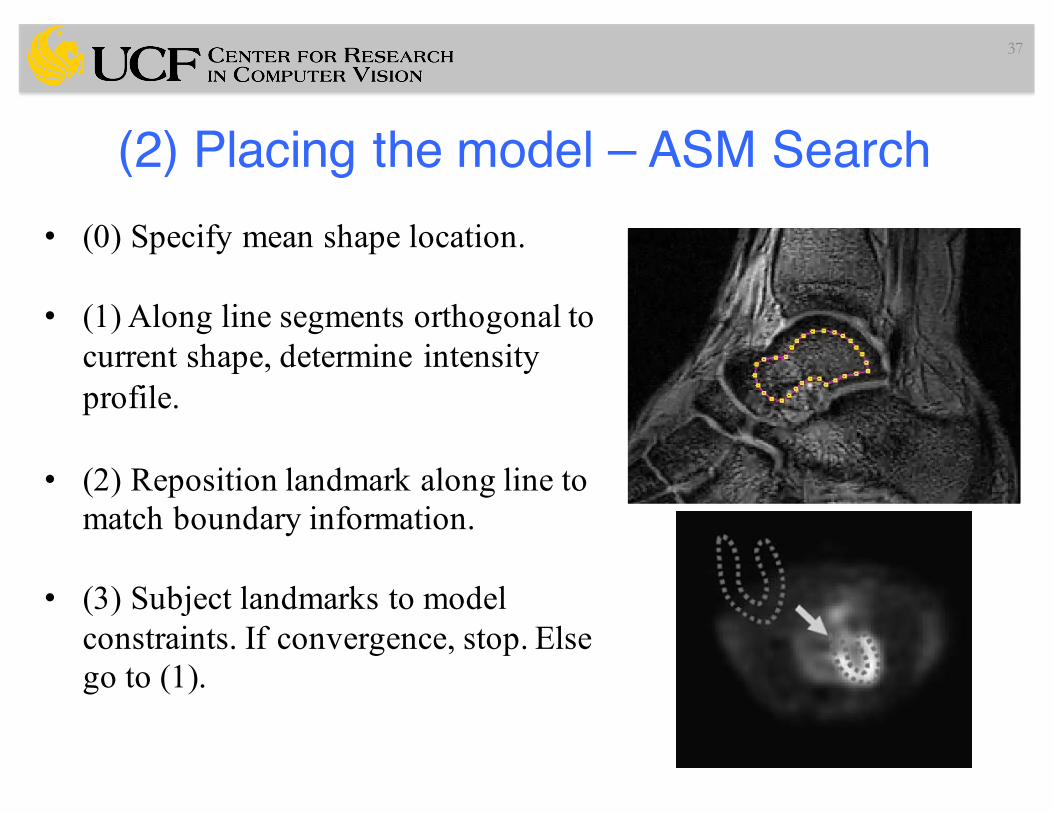
(2) Placing the model – ASM Search• (0) Specify mean shape location.

• (1) Along line segments orthogonal to current shape, determine intensity profile.

• (2) Reposition landmark along line to match boundary information.

• (3) Subject landmarks to model constraints. If convergence, stop. Else go to (1).

37

38

(2) Placing the model – ASM Search),( ii YX

Need to search for local matchFor each point:

-strongest edge-correlation-statistical model of profile

Deeper in ASM Search 39

Model boundary

Model point

Interpolate at these points

,...2,1,0,1,2...

),(),(

−−=

+

insnsiYX ynxn

),( YX

xnns

ynns

ns

),( along length of steps Take yxn nns

)(xg

xdxxdg )(

))1()1((5.0)( −−+= xgxgdxxdg

Select point along profile at strongest edge

Finding the model pose & parameters• Suppose we have identified a set of points Y in the image.

Evidently, we can seek to minimize the squared distance:

Algorithm1. Initialize b=02. Generate initial model instance 3. Find T that best aligns q to Y (e.g., similarity transform)4. Invert pose parameters, to project into model frame5. Update the model parameters: 6. Repeat from step 2 until convergence

40

|Y � T (q̄ +tX

i=1

biui)|2

q = (q̄ +tX

i=1

biui)

y = T�1(Y)

b = UT (y � q̄) U = [u1|u1|...ut]

Example Application: Knee Cartilage quantification - MRI

41

Ex: MR Brain structure segmentation

42

ASM Summary

43

+ Shape prior helps overcoming segmentation errors

+ Fast optimization

+ Can handle interior/exterior dynamics

Pros:

Cons:

Possible improvements:

Learn and apply specific motion priors for different actions

- Optimization gets trapped in local minima

- Re-initialization is problematic

ASM - Problems

44

ASM resultTrue boundary

ASM Problems

45

10 points

20 points

Talus 1 Liver 1

2D landmarking

How about 3D?

Time consuming!CorrespondenceIssue!

Alternative solutions for landmarking• Based on image registration• Based on MDL (min description length) and optimization

techniques• Based on shape characteristics of the objects

46

ASM Problems – Initialization Sensitivity

47

Oriented Active Shape Models (OASM)

48

(1) Selecting landmarks. (2) Building models. (3) Creating boundary cost function. (4) Coarse level recognition. ß(5) Fine level recognition & delineation – 2LDP. ß

training

Overview of Approach

OASM (Liu and Udupa) 49

P3

P1

P2

P4P5

P6

Rec

ogni

tion

Delineation

P1 P2 P6 P1…

- Construct a graph to setup synergy between recgn.and deln.

- Automate recognition.

(5) Fine level recognition & delineation – 2LDP

50

Delineation

P1 P2 P6 P1

Rec

ogni

tion

P1

P2

P3

P4P5

P6



OASM (Liu and Udupa)

51

Rec

ogni

tion

Delineation

P1 P2 P6 P1

P1

P2

P3

P4P5

P6




52OASM (Liu and Udupa)

.

.

.R

ecog

nitio

n

Delineation

P1 P2 P6 P1

P1

P2

P3

P4P5

P6



53

Rec

ogni

tion

Delineation

P1 P2 P6 P1

P1

P2

P3

P4P5

P6




OASM – Recognition (model placement)Coarse level recognition

• At each location in a coarse grid, evaluate the total boundary cost (from Live Wire) via 2LDP by placing the mean shape at that point.

• Select that location for which this total cost is the minimum.

54

OASM – Recognition (model placement)

55

OASM - Segmentation56

Automatic recognition

Final segmentation

Comparison with ASM

57

ASM n=36 OASM n=20

Comparison with ASM

58

OASM n=28ASM n=28

Comparison with ASM

59

OASMASM

Comparison with ASM

60

OASMASM

Comparison with ASM

61

OASMASM

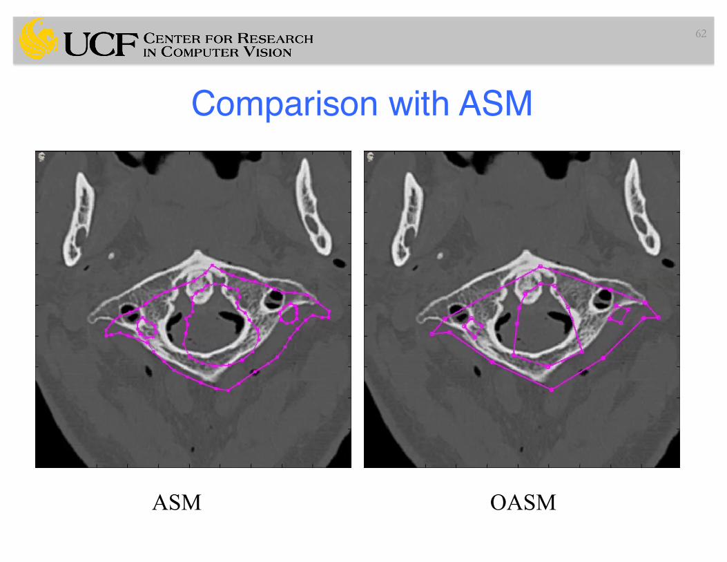
Comparison with ASM

62

OASMASM

Active Appearance Model• PLEASE READ THE FOLLOWING PAPER• T.F.Cootes, G.J. Edwards and C.J.Taylor. "Active Appearance Models",

in Proc. European Conference on Computer Vision 1998 Vol. 2, pp. 484-498, Springer, 1998. (Best paper prize)

63

Summary• Shape

– Shape representation (landmark based)• ASM

– Model placement, ASM search (optimization)• OASM

– Orientedness – Cost function– Less number of landmarks– Improved results

64

Slide Credits and References• Credits to: Jayaram K. Udupa of Univ. of Penn., MIPG• Bagci’s CV Course 2015 Fall.• TF. Cootes et al. ASM and their training and applications,

1995.• S.Pizer (UNC) presentations• K.D. Toennies, Guide to Medical Image Analysis,• Shape Analysis in Medical Image Analysis, Springer.• Handbook of Medical Imaging, Vol. 2. SPIE Press.• Handbook of Biomedical Imaging, Paragios, Duncan, Ayache.

65