lecture 06 marco aurelio ranzato - deep learning
TRANSCRIPT
Deep Learning
Marc'Aurelio Ranzato
Facebook A.I. Research
ICVSS – 15 July 2014www.cs.toronto.edu/~ranzato

https://sites.google.com/site/deeplearningcvpr2014/


6
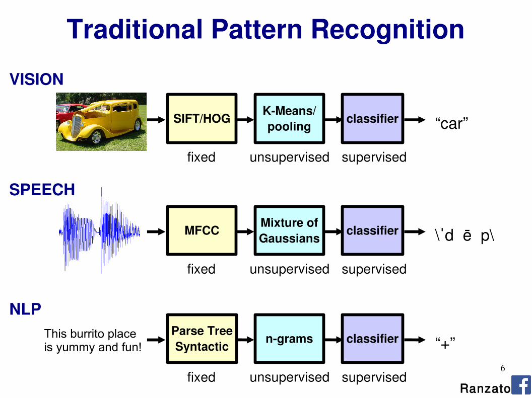
fixed unsupervised supervised
classifierMixture ofGaussians
MFCC \ˈd ē p\
fixed unsupervised supervised
classifierK-Means/poolingSIFT/HOG “car”
fixed unsupervised supervised
classifiern-gramsParse TreeSyntactic “+”
This burrito placeis yummy and fun!
Traditional Pattern Recognition
VISION
SPEECH
NLP
Ranzato

7
Hierarchical Compositionality (DEEP)
VISION
SPEECH
NLP
pixels edge texton motif part object
sample spectral band
formant motif phone word
character NP/VP/.. clause sentence storyword
Ranzato

8
fixed unsupervised supervised
classifierMixture ofGaussians
MFCC \ˈd ē p\
fixed unsupervised supervised
classifierK-Means/poolingSIFT/HOG “car”
fixed unsupervised supervised
classifiern-gramsParse TreeSyntactic “+”
This burrito placeis yummy and fun!
Traditional Pattern Recognition
VISION
SPEECH
NLP
Ranzato

9
Deep Learning
“car”
Cascade of non-linear transformations End to end learning General framework (any hierarchical model is deep)
What is Deep Learning
Ranzato
10
Ranzato
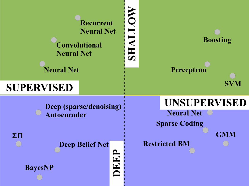
THE SPACE OF MACHINE LEARNING METHODS
11
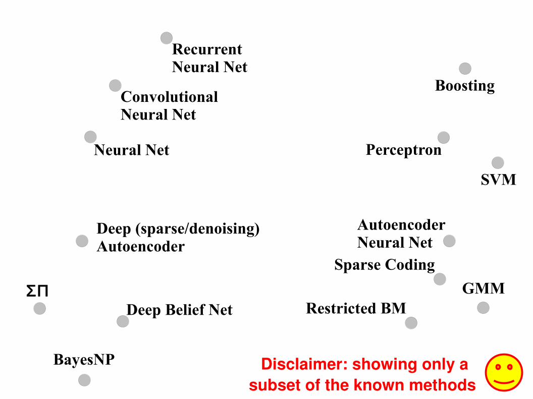
PerceptronNeural Net
Boosting
SVM
GMMΣΠ
BayesNP
Convolutional Neural Net
Recurrent Neural Net
AutoencoderNeural Net
Sparse Coding
Restricted BMDeep Belief Net
Deep (sparse/denoising) Autoencoder
Disclaimer: showing only a subset of the known methods

12
PerceptronNeural Net
Boosting
SVM
GMMΣΠ
BayesNP
Convolutional Neural Net
Recurrent Neural Net
AutoencoderNeural Net
Sparse Coding
Restricted BMDeep Belief Net
Deep (sparse/denoising) Autoencoder
SHA
LL
OW
DE
EP
13
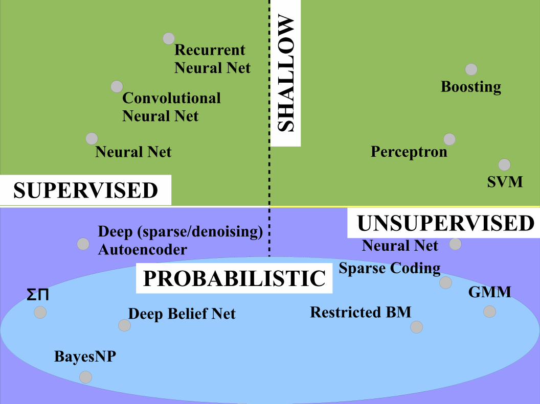
PerceptronNeural Net
Boosting
SVM
GMMΣΠ
BayesNP
Convolutional Neural Net
Recurrent Neural Net
AutoencoderNeural Net
Sparse Coding
Restricted BMDeep Belief Net
Deep (sparse/denoising) Autoencoder
UNSUPERVISED
SUPERVISED
DE
EP
SHA
LL
OW
14
PerceptronNeural Net
Boosting
SVM
Convolutional Neural Net
Recurrent Neural Net
AutoencoderNeural Net
Deep (sparse/denoising) Autoencoder
UNSUPERVISED
SUPERVISED
DE
EP
SHA
LL
OW
ΣΠ
BayesNP
Deep Belief NetGMM
Sparse Coding
Restricted BM
PROBABILISTIC
15
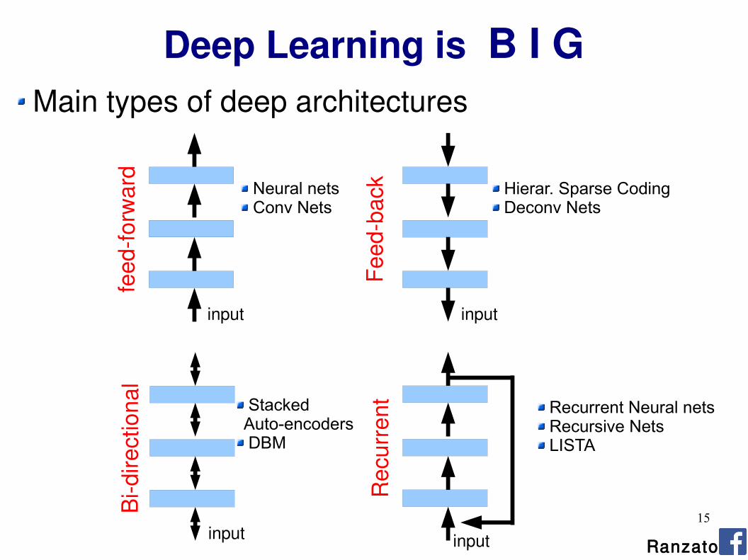
Main types of deep architectures
Ranzato
Deep Learning is B I G
input input
input
feed
-f orw
ard
Feed
- bac
k
Bi-d
irect
ion a
l
Neural nets Conv Nets
Hierar. Sparse Coding Deconv Nets
Stacked Auto-encoders DBM
input
Rec
urre
nt Recurrent Neural nets Recursive Nets LISTA

16
Ranzato
Deep Learning is B I G
input input
input
feed
-f orw
ard
Feed
- bac
k
Bi-d
irect
ion a
l
Neural nets Conv Nets
Hierar. Sparse Coding Deconv Nets
Stacked Auto-encoders DBM
input
Rec
urre
nt Recurrent Neural nets Recursive Nets LISTA
Main types of deep architectures
17
Ranzato
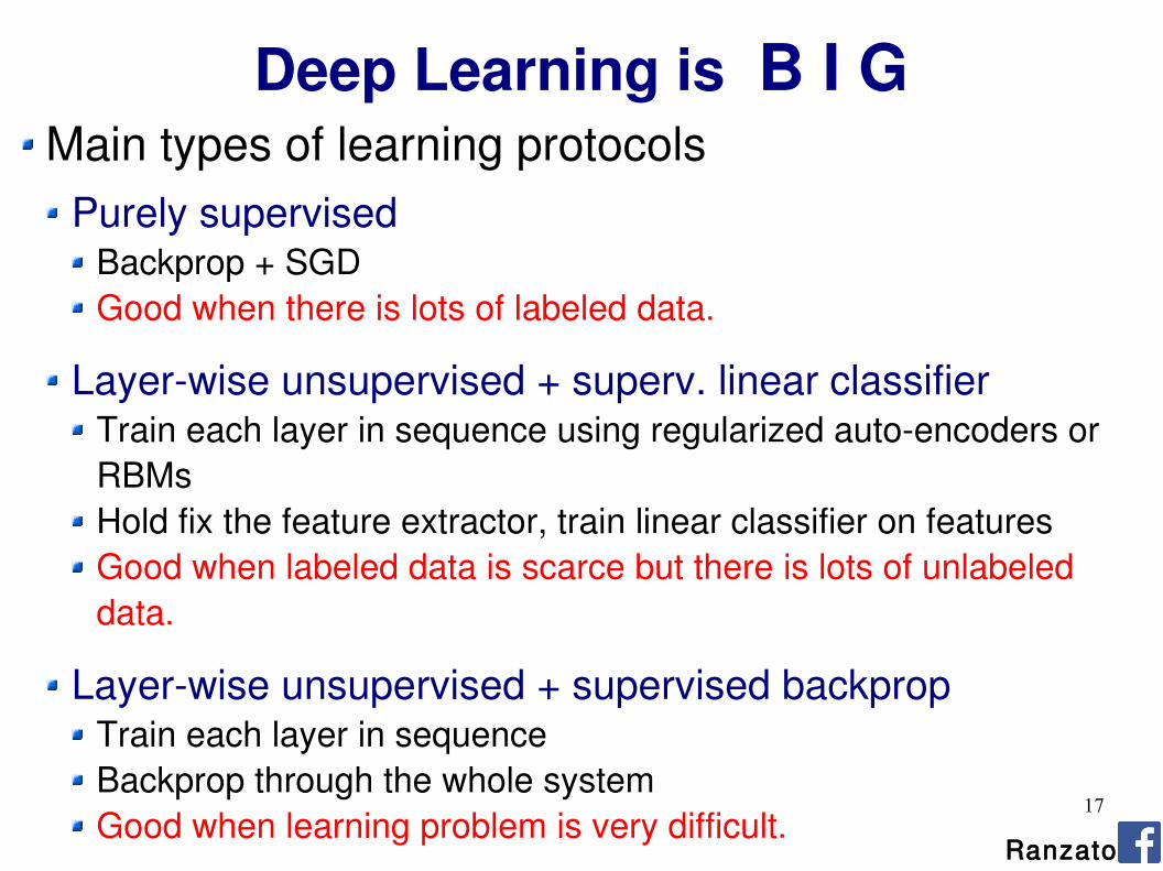
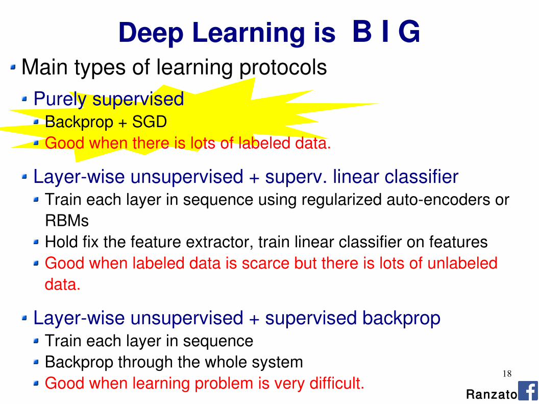
Deep Learning is B I G Main types of learning protocols
Purely supervisedBackprop + SGDGood when there is lots of labeled data.
Layer-wise unsupervised + superv. linear classifierTrain each layer in sequence using regularized auto-encoders or RBMsHold fix the feature extractor, train linear classifier on featuresGood when labeled data is scarce but there is lots of unlabeled data.
Layer-wise unsupervised + supervised backpropTrain each layer in sequenceBackprop through the whole systemGood when learning problem is very difficult.
18
Ranzato
Deep Learning is B I G Main types of learning protocols
Purely supervisedBackprop + SGDGood when there is lots of labeled data.
Layer-wise unsupervised + superv. linear classifierTrain each layer in sequence using regularized auto-encoders or RBMsHold fix the feature extractor, train linear classifier on featuresGood when labeled data is scarce but there is lots of unlabeled data.
Layer-wise unsupervised + supervised backpropTrain each layer in sequenceBackprop through the whole systemGood when learning problem is very difficult.
19
Outline Part I
Ranzato
Supervised Neural Networks
Convolutional Neural Networks
Examples
Tips

20
Neural Networks
Ranzato
Assumptions (for the next few slides): The input image is vectorized (disregard the spatial layout of pixels) The target label is discrete (classification)
Question: what class of functions shall we consider to map the input into the output?
Answer: composition of simpler functions.
Follow-up questions: Why not a linear combination? What are the “simpler” functions? What is the interpretation?
Answer: later...
21
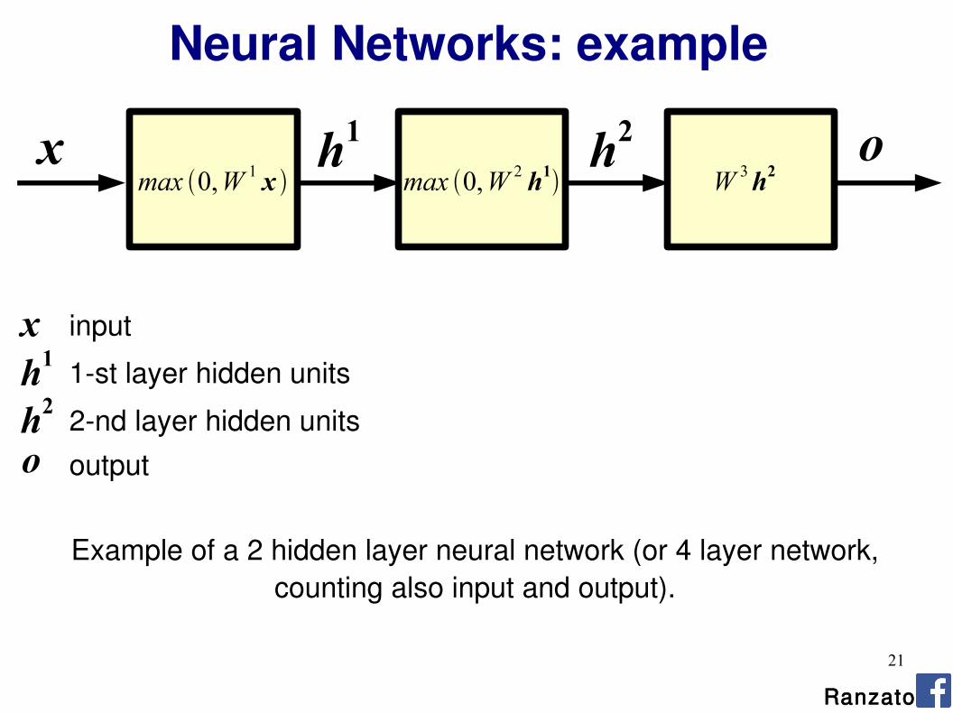
Neural Networks: example
h2h1xmax 0,W 1 x max 0,W 2 h1
W 3h2
Ranzato
input
1-st layer hidden units
2-nd layer hidden units output
Example of a 2 hidden layer neural network (or 4 layer network, counting also input and output).
xh1
h2
o
o
22
Forward Propagation
Ranzato
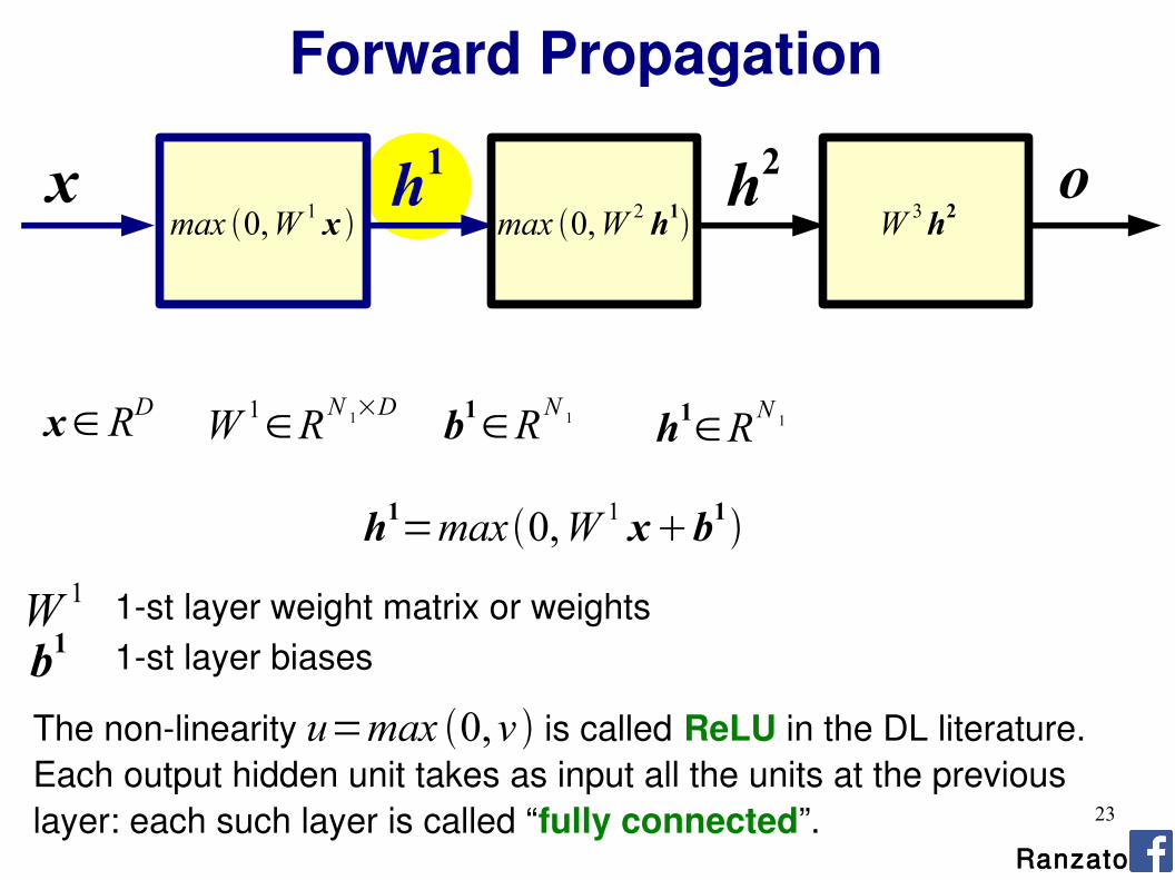
Def.: Forward propagation is the process of computing the output of the network given its input.
23
Forward Propagation
Ranzato
h1=max0,W 1 xb1
x∈RDW 1
∈RN 1×D b1
∈RN 1 h1
∈RN 1
x
1-st layer weight matrix or weightsW 1
1-st layer biasesb1
o
The non-linearity is called ReLU in the DL literature.Each output hidden unit takes as input all the units at the previous layer: each such layer is called “fully connected”.
u=max 0,v
h2h1
max 0,W 1 x max 0,W 2 h1 W 3h2

24
Forward Propagation
Ranzato
h2=max 0,W 2h1b2
h1∈R
N 1 W 2∈R
N 2×N 1 b2∈R
N 2 h2∈R
N 2
x o
2-nd layer weight matrix or weightsW 2
2-nd layer biasesb2
h2h1
max 0,W 1 x max 0,W 2 h1 W 3h2

25
Forward Propagation
Ranzato
o=max 0,W 3h2b3
h2∈R
N 2 W 3∈R
N 3×N 2 b3∈R
N 3 o∈RN 3
x o
3-rd layer weight matrix or weightsW 3
3-rd layer biasesb3
h2h1
max 0,W 1 x max 0,W 2 h1 W 3h2
26
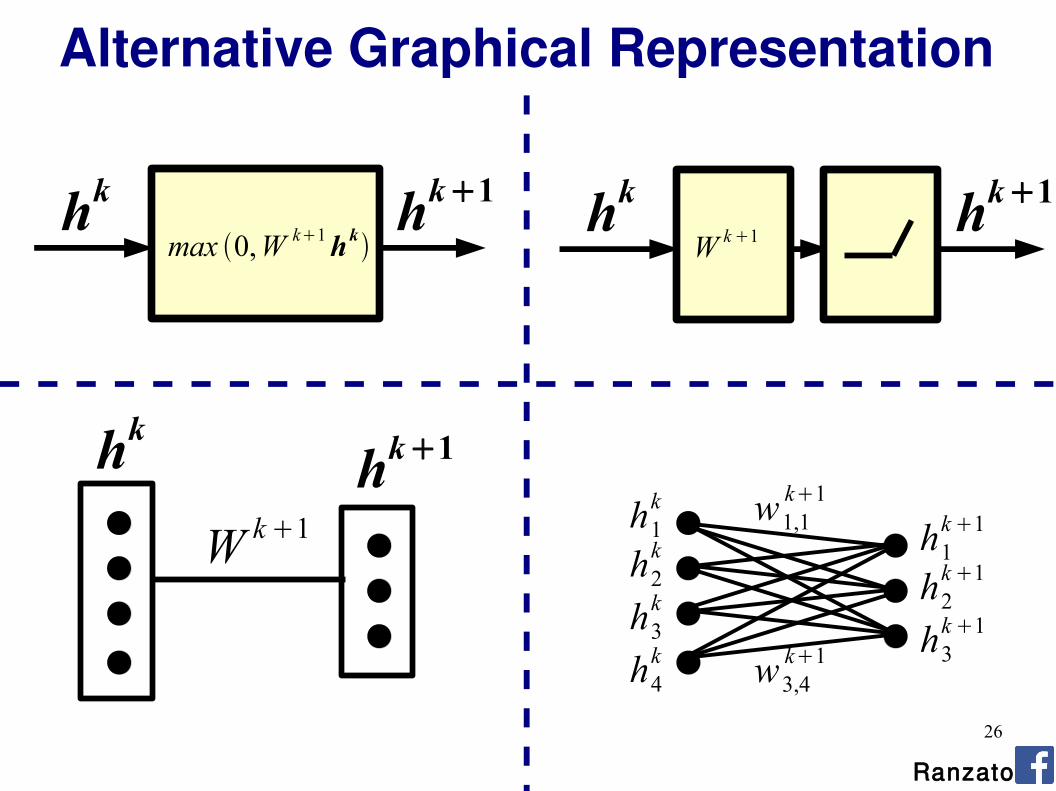
Alternative Graphical Representation
Ranzato
hk1hkmax 0,W k1hk
hk1hkW k1
h1k
h2k
h3k
h4k
h1k1
h2k1
h3k1
w1,1k1
w3,4k1
hk hk1
W k1

27
Interpretation
Ranzato
Question: Why can't the mapping between layers be linear?
Answer: Because composition of linear functions is a linear function. Neural network would reduce to (1 layer) logistic regression.
Question: What do ReLU layers accomplish?
Answer: Piece-wise linear tiling: mapping is locally linear.
Montufar et al. “On the number of linear regions of DNNs” arXiv 2014

28
Ranzato
[0/1]
[0/1]
[0/1]
[0/1] [0/1]
[0/1]
[0/1]
[0/1]
ReLU layers do local linear approximation. Number of planes grows exponentially with number of hidden units. Multiple layers yeild exponential savings in number of parameters (parameter sharing).
Montufar et al. “On the number of linear regions of DNNs” arXiv 2014
29
Interpretation
Ranzato
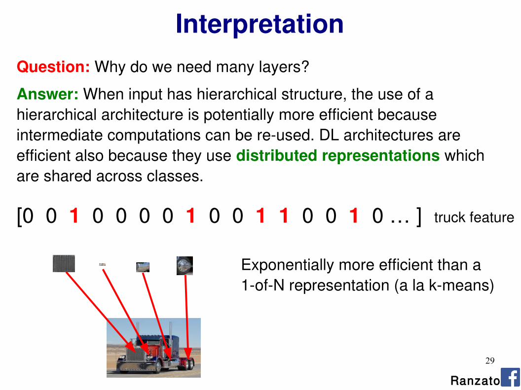
Question: Why do we need many layers?
Answer: When input has hierarchical structure, the use of a hierarchical architecture is potentially more efficient because intermediate computations can be re-used. DL architectures are efficient also because they use distributed representations which are shared across classes.
[0 0 1 0 0 0 0 1 0 0 1 1 0 0 1 0 … ]
Exponentially more efficient than a 1-of-N representation (a la k-means)
truck feature

30
Interpretation
Ranzato
[0 0 1 0 0 0 0 1 0 0 1 1 0 0 1 0 … ]
[1 1 0 0 0 1 0 1 0 0 0 0 1 1 0 1… ] motorbike
truck

31
Interpretation
Ranzato
Input image
low level parts
prediction of class
mid-level parts
high-level parts
distributed representations feature sharing compositionality
...
Lee et al. “Convolutional DBN's ...” ICML 2009

32
Interpretation
Ranzato
Question: How many layers? How many hidden units?
Answer: Cross-validation or hyper-parameter search methods are the answer. In general, the wider and the deeper the network the more complicated the mapping.
Question: What does a hidden unit do?
Answer: It can be thought of as a classifier or feature detector.
Question: How do I set the weight matrices?
Answer: Weight matrices and biases are learned.First, we need to define a measure of quality of the current mapping.Then, we need to define a procedure to adjust the parameters.

33
h2h1x o
Loss
max 0,W 1 x max 0,W 2 h1 W 3h2
L x , y ; =−∑ jy j log p c j∣x
pck=1∣x =eo k
∑ j=1
Ceo j
Probability of class k given input (softmax):
(Per-sample) Loss; e.g., negative log-likelihood (good for classification of small number of classes):
Ranzato
How Good is a Network?
y=[00 .. 010 .. 0 ]k1 C
34
Training
∗=arg min∑n=1
PL x n , yn ;
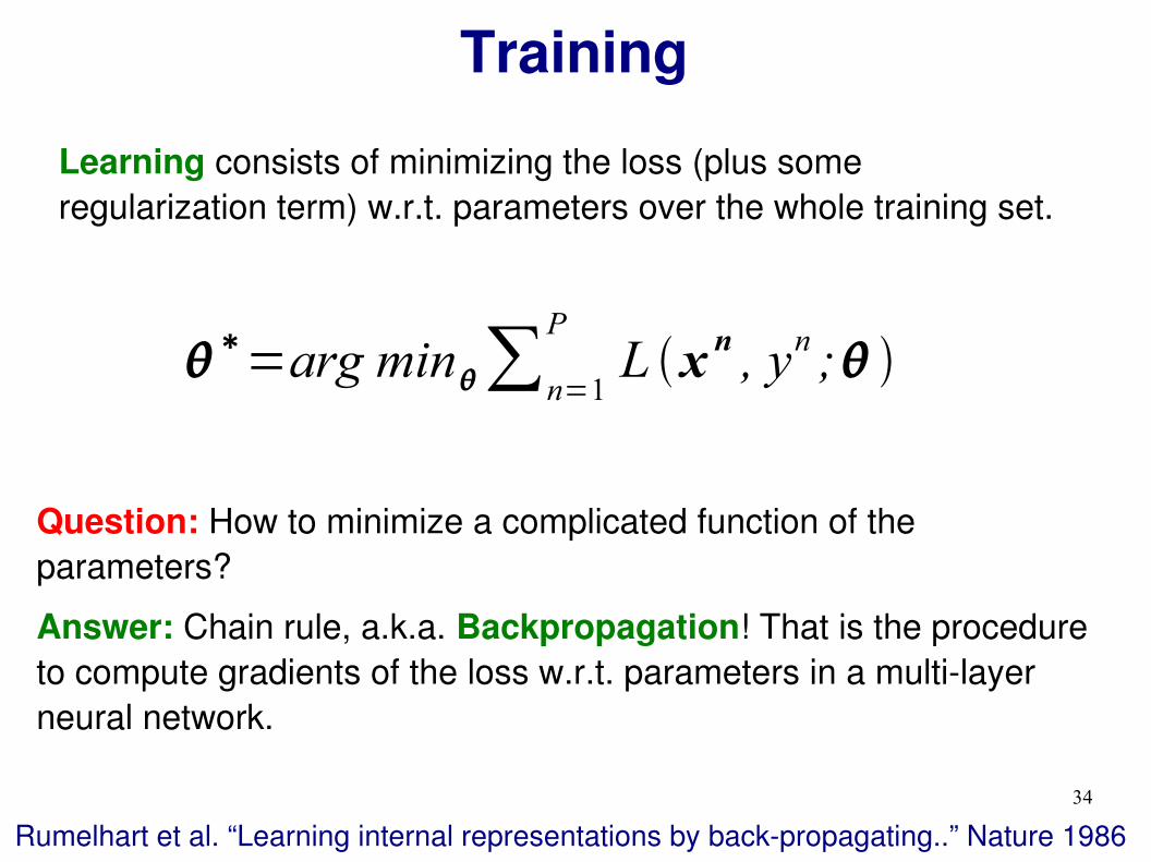
Learning consists of minimizing the loss (plus some regularization term) w.r.t. parameters over the whole training set.
Question: How to minimize a complicated function of the parameters?
Answer: Chain rule, a.k.a. Backpropagation! That is the procedure to compute gradients of the loss w.r.t. parameters in a multi-layer neural network.
Rumelhart et al. “Learning internal representations by back-propagating..” Nature 1986
35
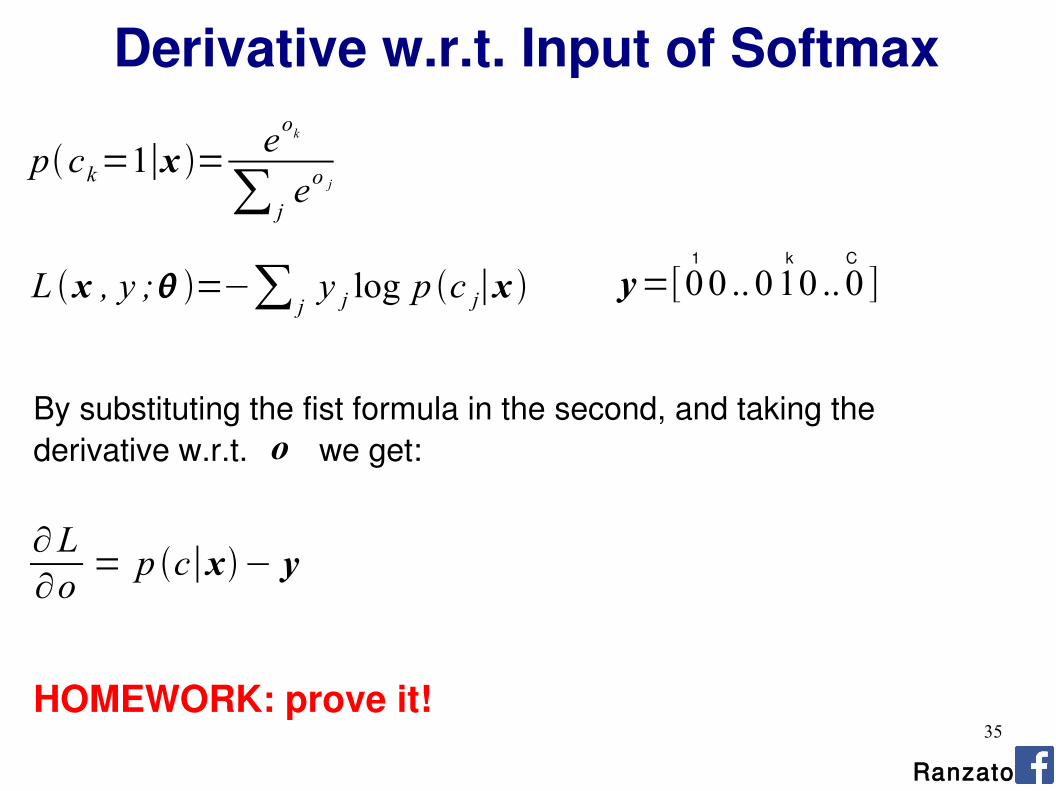
Derivative w.r.t. Input of Softmax
L x , y ; =−∑ jy j log p c j∣x
pck=1∣x =eok
∑ jeo j
By substituting the fist formula in the second, and taking the derivative w.r.t. we get:o
∂L∂o
= p c∣x− y
HOMEWORK: prove it!
Ranzato
y=[00 .. 010 .. 0 ]k1 C

36
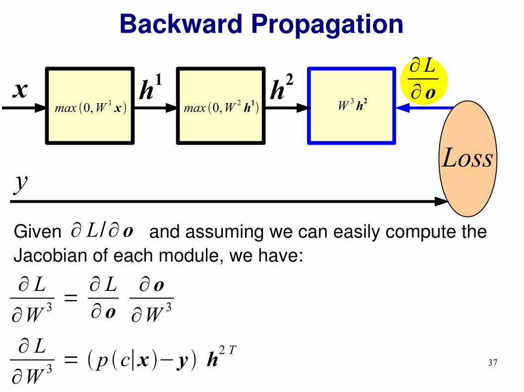
Backward Propagation
h2h1x
Lossy
Given and assuming we can easily compute the Jacobian of each module, we have:
∂ L/∂ o
∂L∂ o
max 0,W 1 x max 0,W 2 h1 W 3h2
∂ L
∂W 3 =∂ L∂ o
∂ o
∂W 3
37
Backward Propagation
h2h1x
Lossy
Given and assuming we can easily compute the Jacobian of each module, we have:
∂ L/∂ o
∂ L
∂W 3 =∂ L∂ o
∂ o
∂W 3
∂L∂ o
max 0,W 1 x max 0,W 2 h1 W 3h2
∂ L
∂W 3 = p c∣x − y h2 T

38
Backward Propagation
h2h1x
Lossy
Given and assuming we can easily compute the Jacobian of each module, we have:
∂ L/∂ o
∂ L
∂h2=
∂ L∂ o
∂ o
∂h2∂ L
∂W 3 =∂ L∂ o
∂ o
∂W 3
∂L∂ o
max 0,W 1 x max 0,W 2 h1 W 3h2
∂ L
∂W 3 = p c∣x − y h2 T

39
Backward Propagation
h2h1x
Lossy
Given and assuming we can easily compute the Jacobian of each module, we have:
∂ L/∂ o
∂ L
∂h2=
∂ L∂ o
∂ o
∂h2∂ L
∂W 3 =∂ L∂ o
∂ o
∂W 3
∂L∂ o
max 0,W 1 x max 0,W 2 h1 W 3h2
∂ L
∂W 3 = p c∣x − y h2 T ∂ L
∂h2= W
3 T pc∣x − y
40
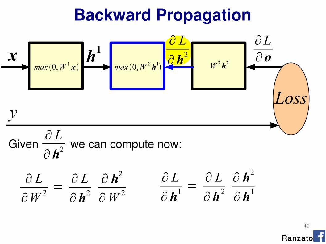
Backward Propagation
h1x
Lossy
Given we can compute now:∂ L
∂h2
∂ L
∂h1=
∂ L
∂h2∂ h2
∂h1∂ L
∂W 2 =∂ L
∂h2∂ h2
∂W 2
∂L∂ o
∂ L
∂h2
Ranzato
max 0,W 1 x max 0,W 2 h1 W 3h2
41
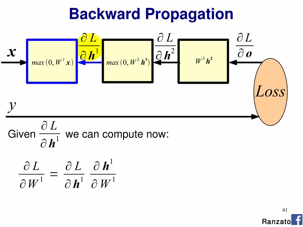
Backward Propagation
x
Lossy
Given we can compute now:∂ L
∂h1
∂ L
∂W 1 =∂ L
∂h1∂ h1
∂W 1
∂ L
∂h1
Ranzato
max 0,W 1 x max 0,W 2 h1
∂L∂ o
∂ L
∂h2W 3h2
42
Backward Propagation
Ranzato
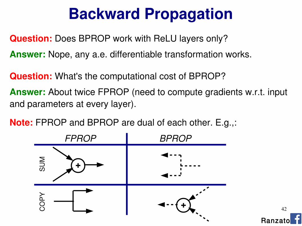
Question: Does BPROP work with ReLU layers only?
Answer: Nope, any a.e. differentiable transformation works.
Question: What's the computational cost of BPROP?
Answer: About twice FPROP (need to compute gradients w.r.t. input and parameters at every layer).
Note: FPROP and BPROP are dual of each other. E.g.,:
+
+
FPROP BPROP
SU
MC
OP
Y
43
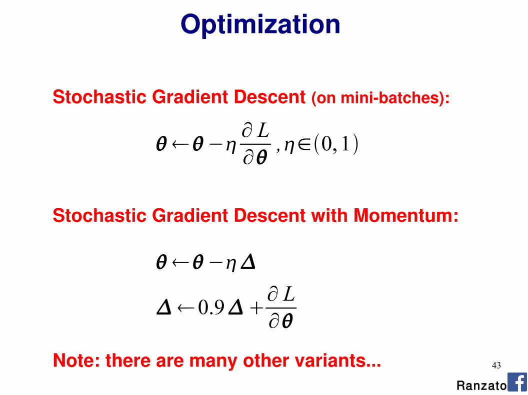
Optimization
Stochastic Gradient Descent (on mini-batches):
−∂ L∂
,∈0,1
Stochastic Gradient Descent with Momentum:
0.9∂ L∂
−
RanzatoNote: there are many other variants...

44
Outline
Ranzato
Supervised Neural Networks
Convolutional Neural Networks
Examples
Tips

45
Example: 200x200 image 40K hidden units
~2B parameters!!!
- Spatial correlation is local- Waste of resources + we have not enough training samples anyway..
Fully Connected Layer
Ranzato
46
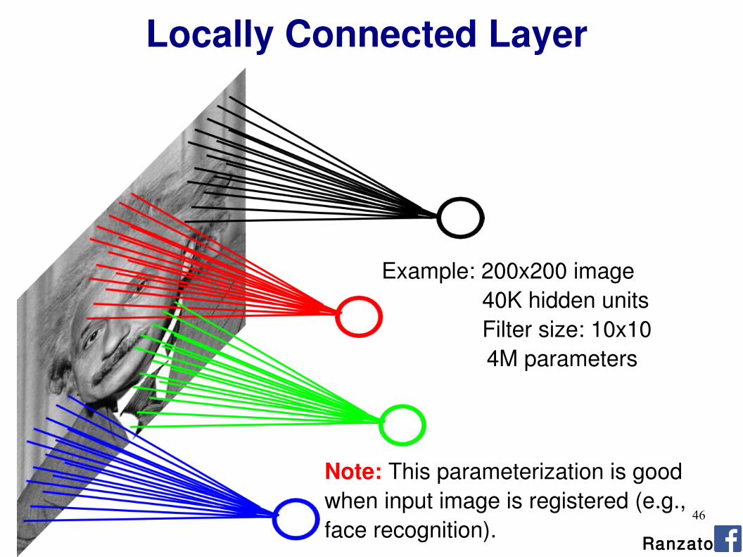
Locally Connected Layer
Example: 200x200 image 40K hidden units Filter size: 10x10
4M parameters
Ranzato
Note: This parameterization is good when input image is registered (e.g., face recognition).
47
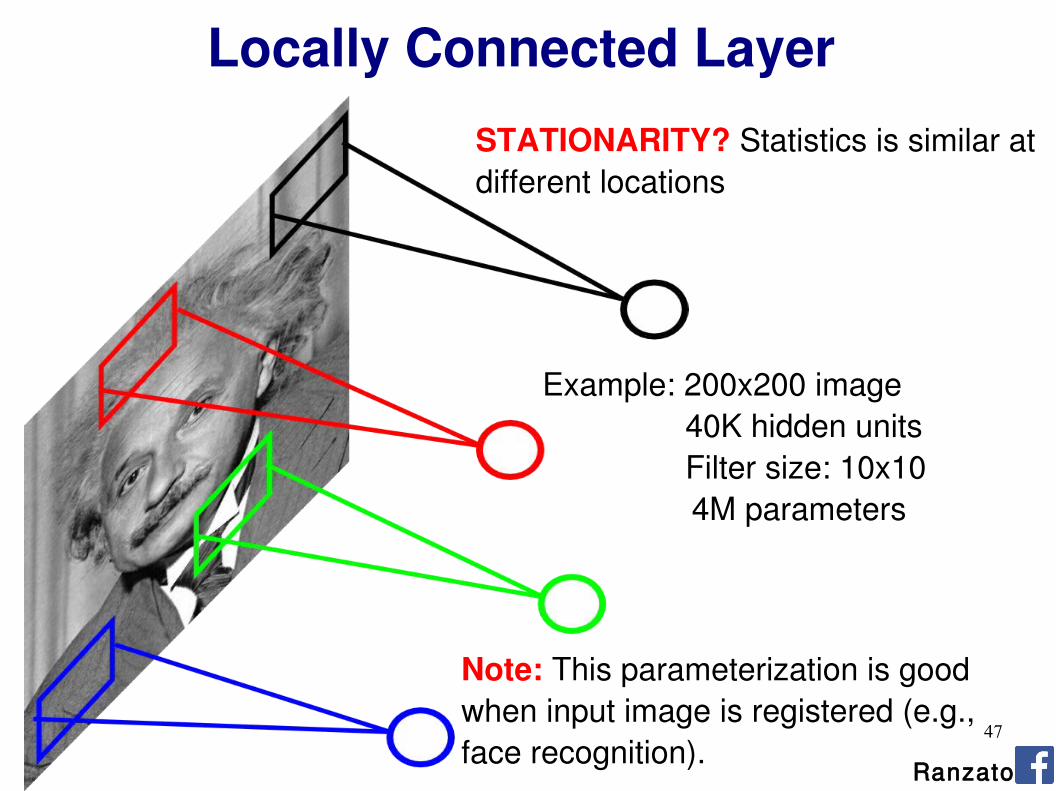
STATIONARITY? Statistics is similar at different locations
Ranzato
Note: This parameterization is good when input image is registered (e.g., face recognition).
Locally Connected Layer
Example: 200x200 image 40K hidden units Filter size: 10x10
4M parameters

48
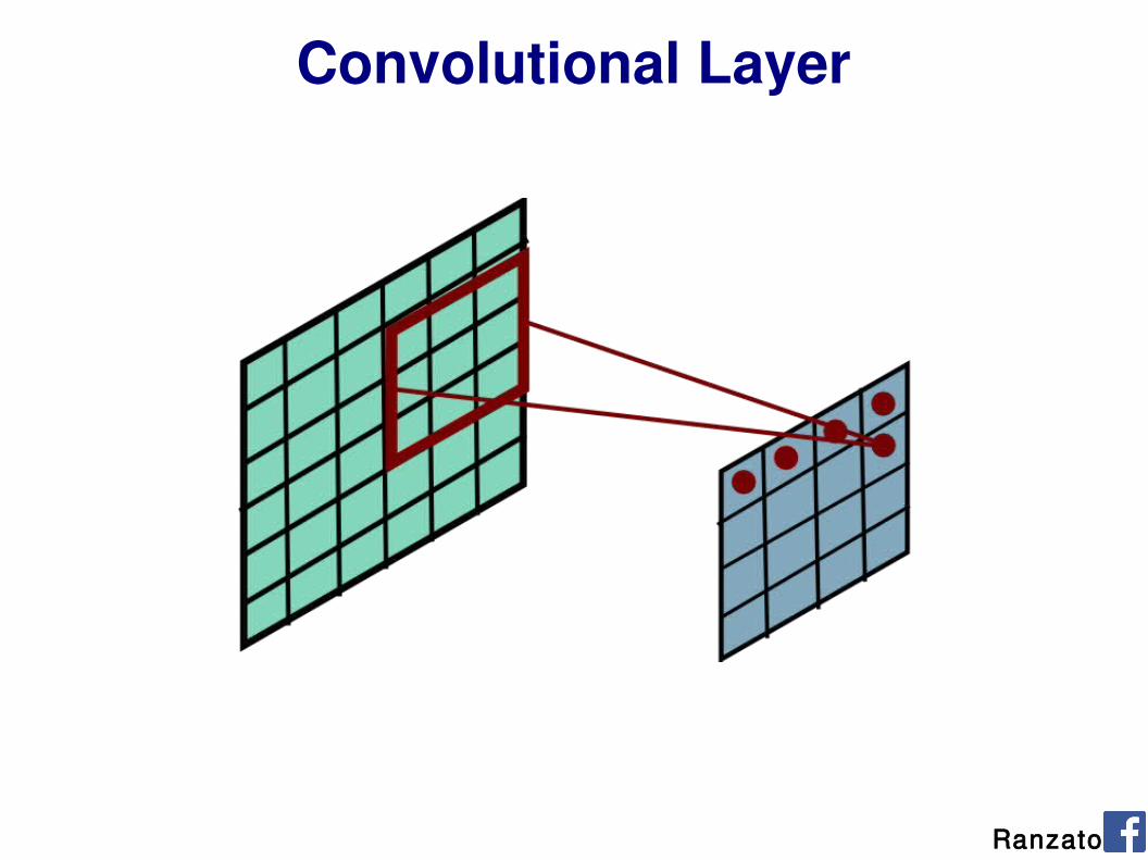
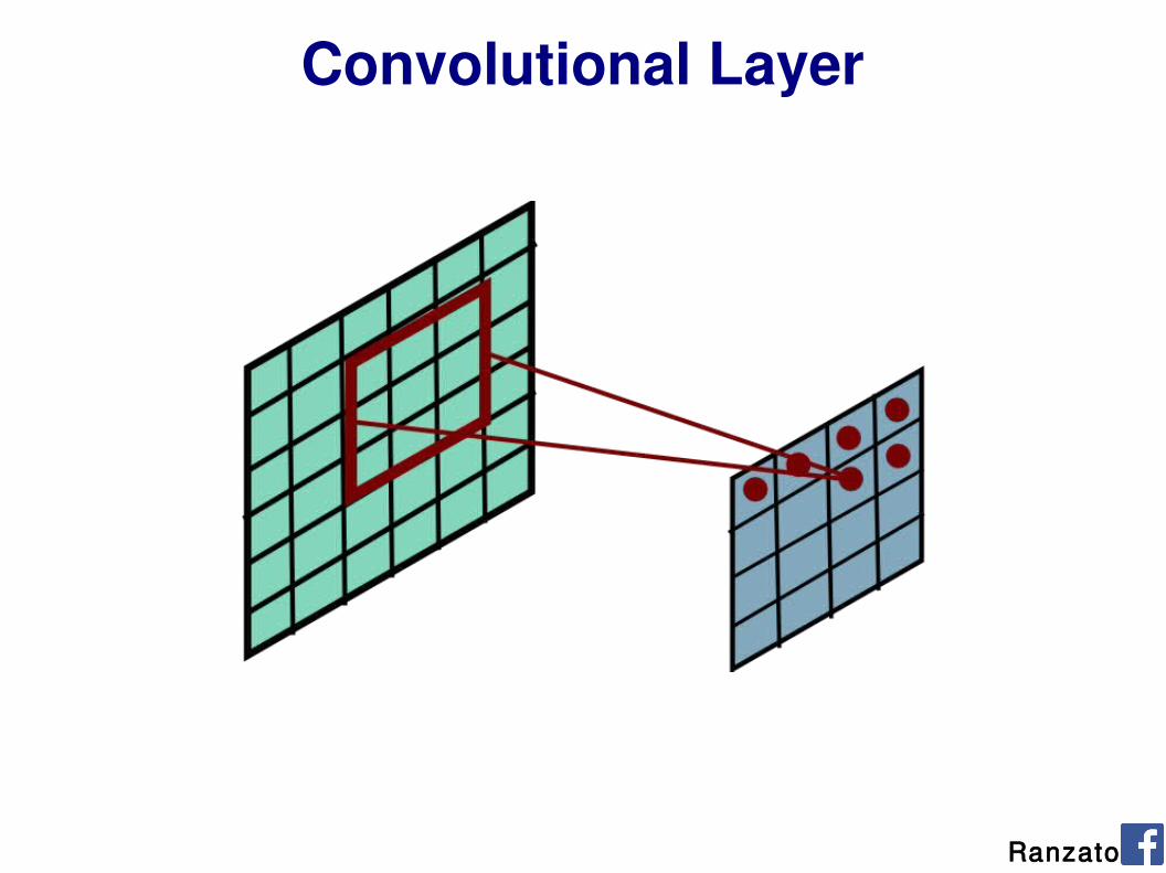
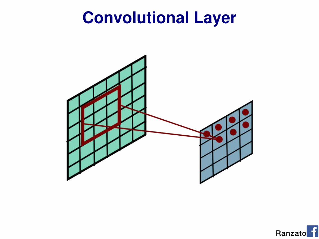
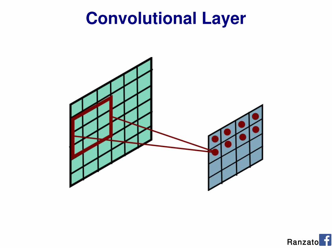
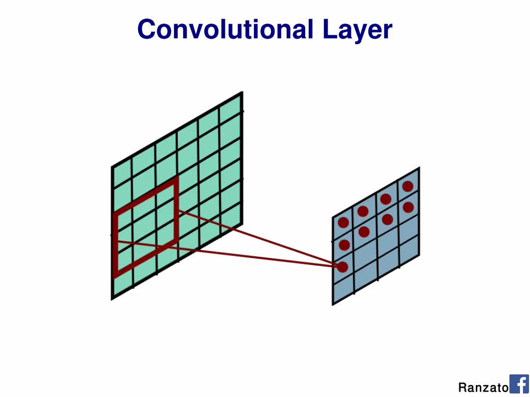
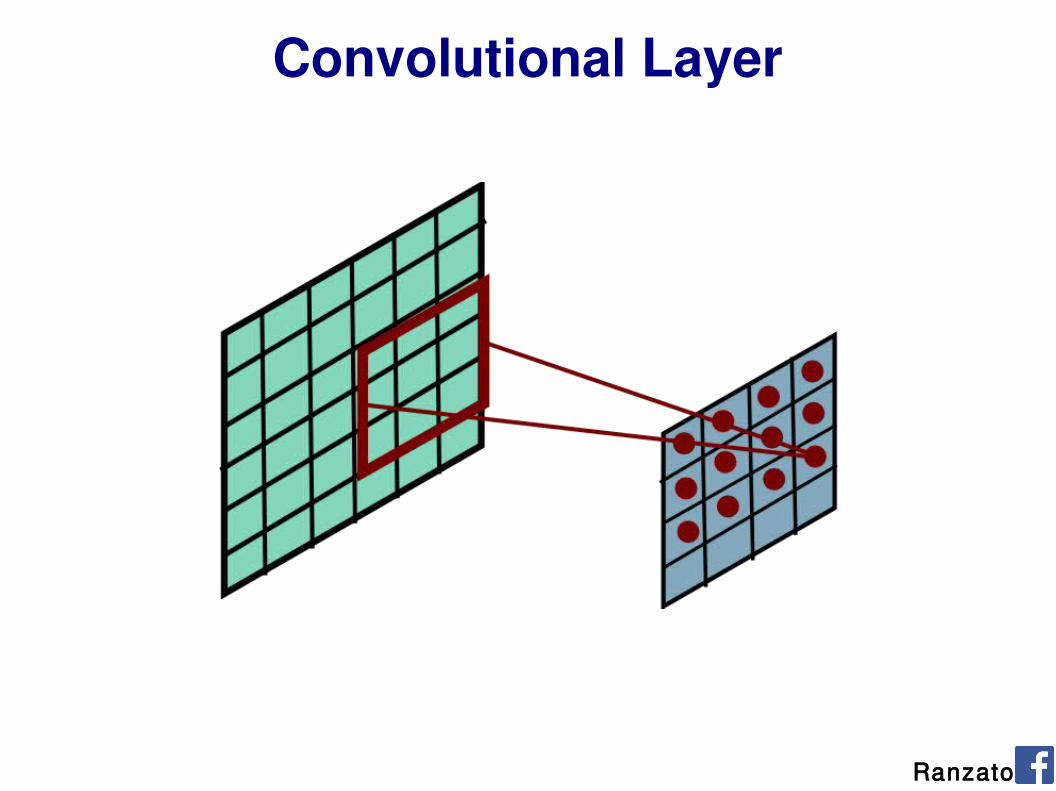
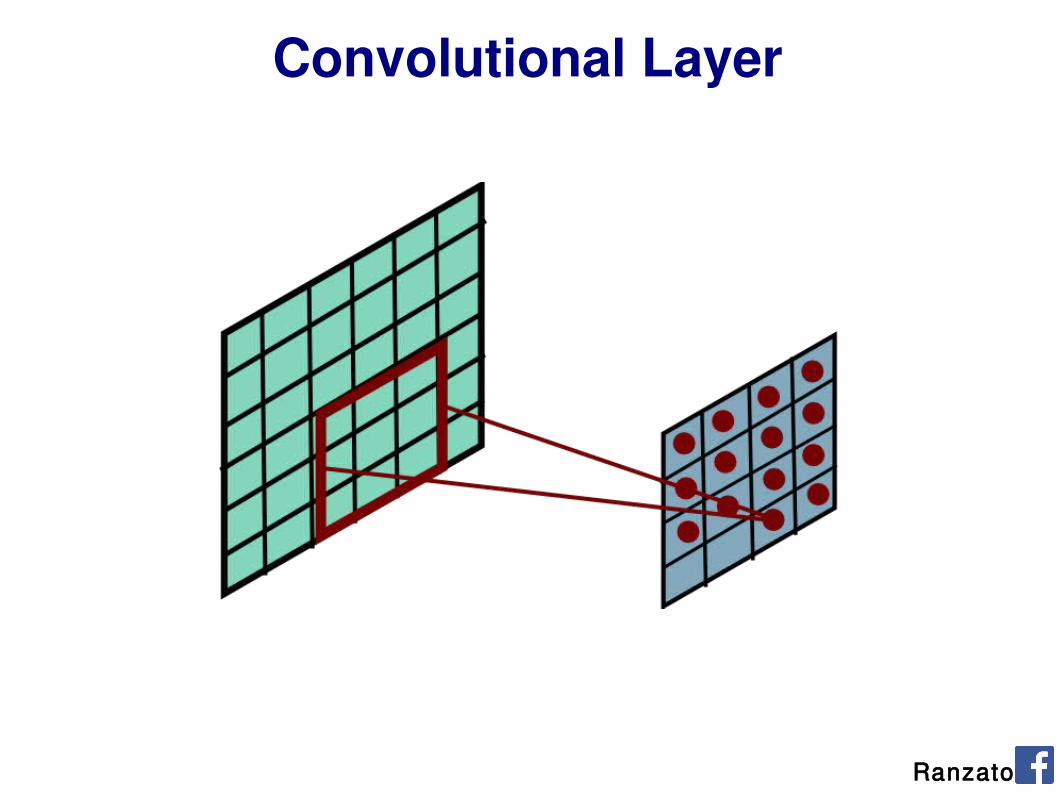
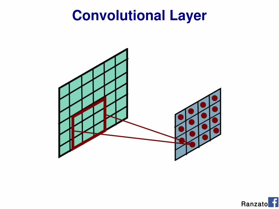
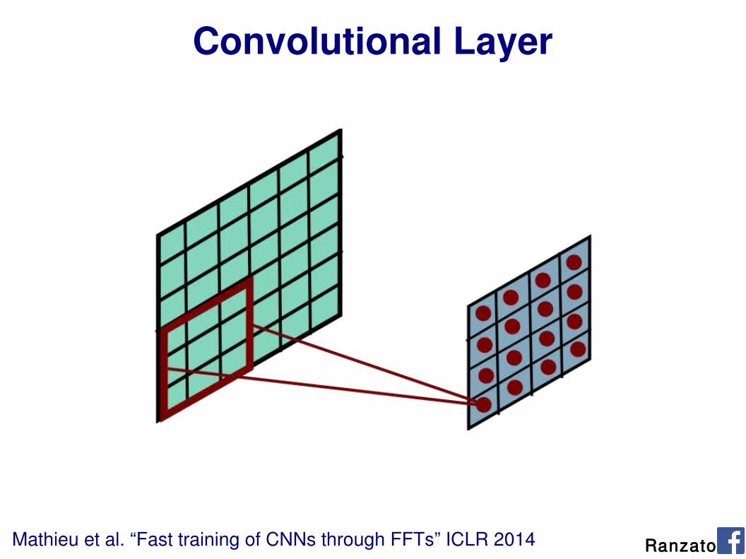
Convolutional Layer
Share the same parameters across different locations (assuming input is stationary):Convolutions with learned kernels
Ranzato

Convolutional Layer
Ranzato

Convolutional Layer
Ranzato

Convolutional Layer
Ranzato

Convolutional Layer
Ranzato
Convolutional Layer
Ranzato
Convolutional Layer
Ranzato
Convolutional Layer
Ranzato
Convolutional Layer
Ranzato
Convolutional Layer
Ranzato

Convolutional Layer
Ranzato

Convolutional Layer
Ranzato
Convolutional Layer
Ranzato

Convolutional Layer
Ranzato
Convolutional Layer
Ranzato
Convolutional Layer
Ranzato
Convolutional Layer
RanzatoMathieu et al. “Fast training of CNNs through FFTs” ICLR 2014
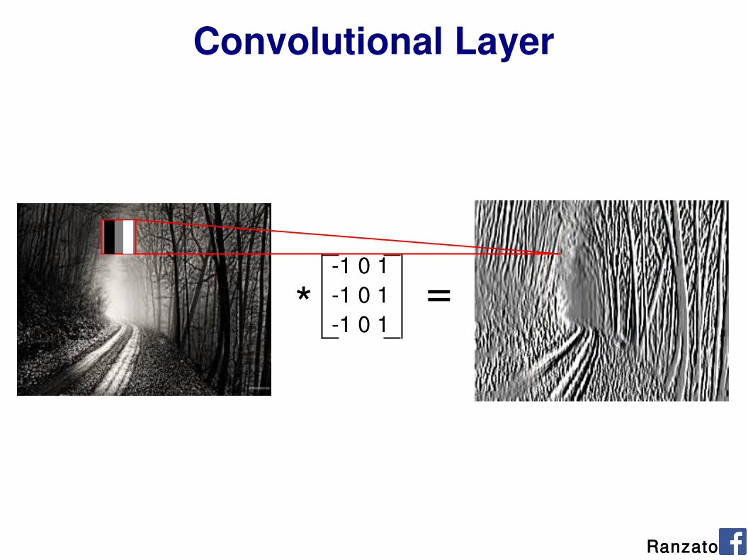
Convolutional Layer
*
-1 0 1-1 0 1-1 0 1
Ranzato
=
66
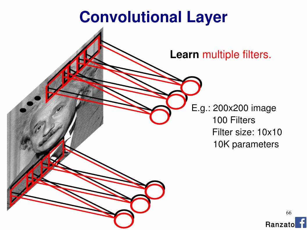
Learn multiple filters.
E.g.: 200x200 image 100 Filters Filter size: 10x10
10K parameters
Ranzato
Convolutional Layer
67
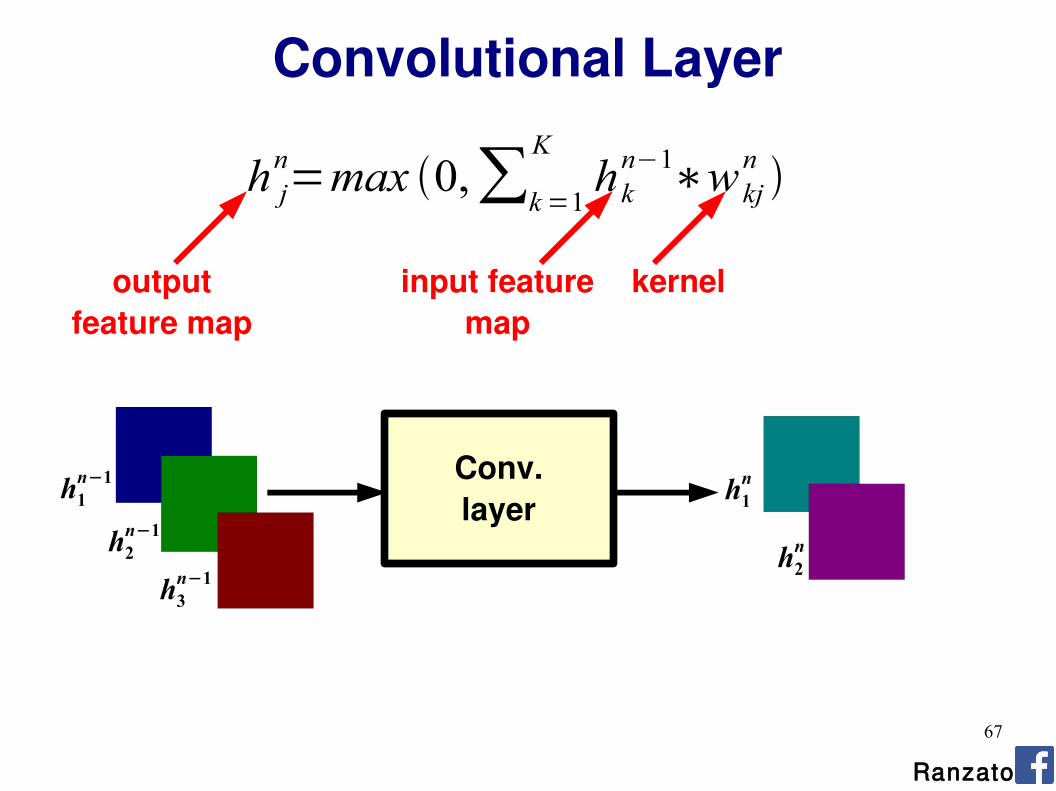
h jn=max 0,∑k=1
Khkn−1∗w kj
n
Ranzato
Conv.layer
h1n−1
h2n−1
h3n−1
h1n
h2n
output feature map
input feature map
kernel
Convolutional Layer

68
h jn=max 0,∑k=1
Khkn−1∗w kj
n
Ranzato
h1n−1
h2n−1
h3n−1
h1n
h2n
output feature map
input feature map
kernel
Convolutional Layer

69
h jn=max 0,∑k=1
Khkn−1∗w kj
n
Ranzato
h1n−1
h2n−1
h3n−1
h1n
h2n
output feature map
input feature map
kernel
Convolutional Layer

70
Ranzato
Question: What is the size of the output? What's the computational cost?
Answer: It is proportional to the number of filters and depends on the stride. If kernels have size KxK, input has size DxD, stride is 1, and there are M input feature maps and N output feature maps then:- the input has size M@DxD - the output has size N@(D-K+1)x(D-K+1)- the kernels have MxNxKxK coefficients (which have to be learned)- cost: M*K*K*N*(D-K+1)*(D-K+1)
Question: How many feature maps? What's the size of the filters?
Answer: Usually, there are more output feature maps than input feature maps. Convolutional layers can increase the number of hidden units by big factors (and are expensive to compute).The size of the filters has to match the size/scale of the patterns we want to detect (task dependent).
Convolutional Layer

71
A standard neural net applied to images:
- scales quadratically with the size of the input- does not leverage stationarity
Solution:
- connect each hidden unit to a small patch of the input- share the weight across spaceThis is called: convolutional layer.A network with convolutional layers is called convolutional network.
LeCun et al. “Gradient-based learning applied to document recognition” IEEE 1998
Key Ideas
72
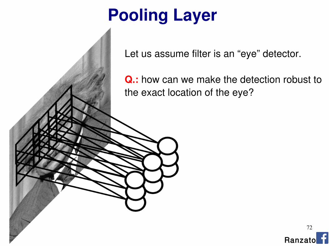
Let us assume filter is an “eye” detector.
Q.: how can we make the detection robust to the exact location of the eye?
Pooling Layer
Ranzato

73
By “pooling” (e.g., taking max) filterresponses at different locations we gainrobustness to the exact spatial locationof features.
Ranzato
Pooling Layer

74
Ranzato
Pooling Layer: Examples
h jn x , y =max
x∈N x , y∈N y h jn−1x ,y
Max-pooling:
h jn x , y =1/K∑
x∈N x , y∈N yh jn−1x ,y
Average-pooling:
h jn x , y =∑x∈N x , y∈N y
h jn−1
x ,y 2
L2-pooling:
h jn x , y =∑k∈N j
hkn−1 x , y 2
L2-pooling over features:

75
Ranzato
Pooling LayerQuestion: What is the size of the output? What's the computational cost?
Answer: The size of the output depends on the stride between the pools. For instance, if pools do not overlap and have size KxK, and the input has size DxD with M input feature maps, then:- output is M@(D/K)x(D/K)- the computational cost is proportional to the size of the input (negligible compared to a convolutional layer)
Question: How should I set the size of the pools?
Answer: It depends on how much “invariant” or robust to distortions we want the representation to be. It is best to pool slowly (via a few stacks of conv-pooling layers).
76
Ranzato
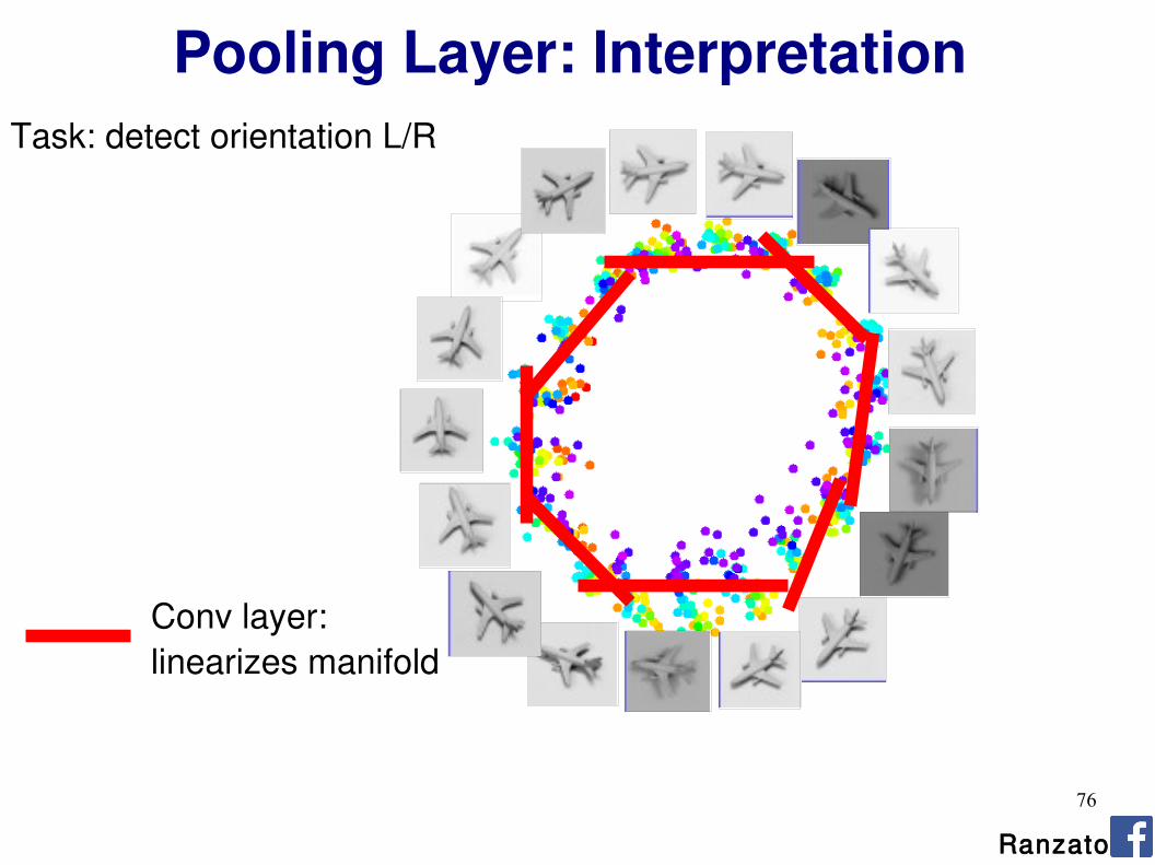
Pooling Layer: InterpretationTask: detect orientation L/R
Conv layer: linearizes manifold
77
Ranzato
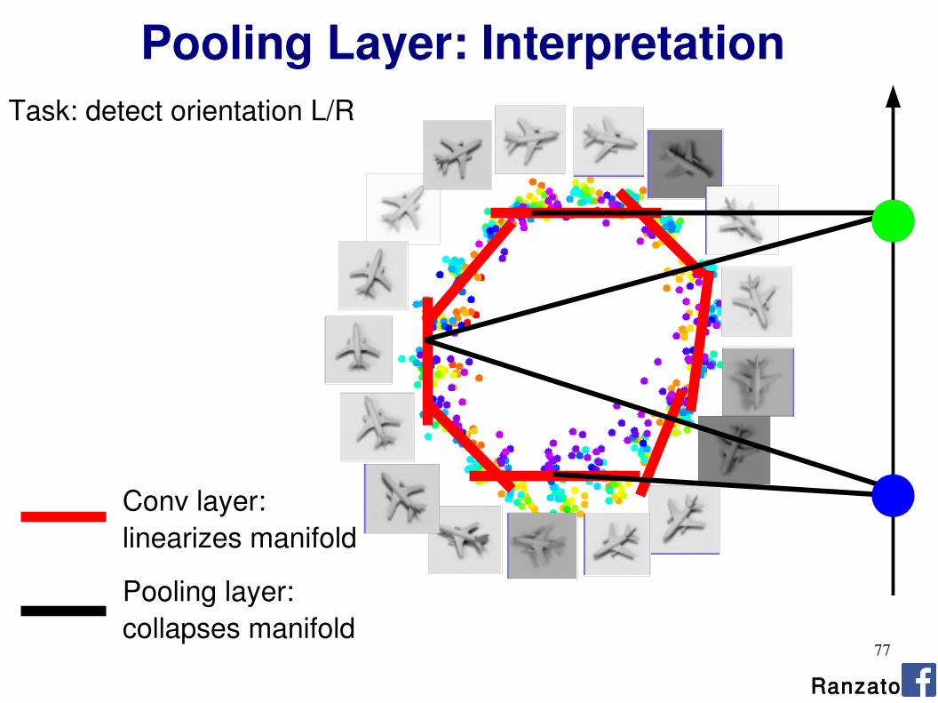
Pooling Layer: Interpretation
Conv layer: linearizes manifold
Pooling layer: collapses manifold
Task: detect orientation L/R

78
Ranzato
Pooling Layer: Receptive Field Size
Conv.layer
hn−1 hn
Pool.layer
hn1
If convolutional filters have size KxK and stride 1, and pooling layer has pools of size PxP, then each unit in the pooling layer depends upon a patch (at the input of the preceding conv. layer) of size: (P+K-1)x(P+K-1)

79
Ranzato
Pooling Layer: Receptive Field Size
Conv.layer
hn−1 hn
Pool.layer
hn1
If convolutional filters have size KxK and stride 1, and pooling layer has pools of size PxP, then each unit in the pooling layer depends upon a patch (at the input of the preceding conv. layer) of size: (P+K-1)x(P+K-1)
80
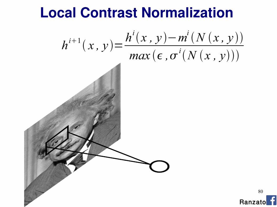
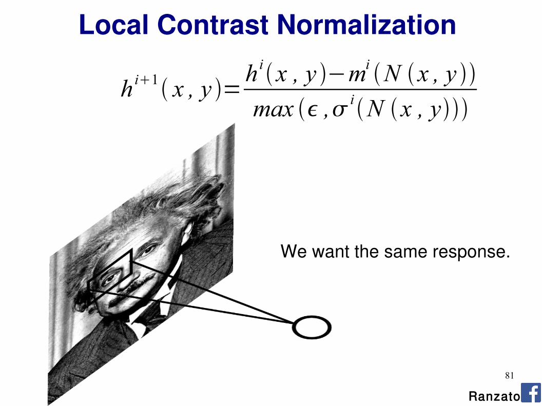
Local Contrast Normalization
h i1 x , y =h ix , y −mi
N x , y
max , iN x , y
Ranzato
81
We want the same response.
Ranzato
Local Contrast Normalization
h i1 x , y =h ix , y −mi
N x , y
max , iN x , y

82
Performed also across features and in the higher layers..
Effects:– improves invariance– improves optimization– increases sparsity
Note: computational cost is negligible w.r.t. conv. layer.
Ranzato
Local Contrast Normalization
h i1 x , y =h ix , y −mi
N x , y
max , iN x , y

83
ConvNets: Typical Stage
Convol. LCN Pooling
One stage (zoom)
courtesy of K. Kavukcuoglu Ranzato

84
Convol. LCN Pooling
One stage (zoom)
Conceptually similar to: SIFT, HoG, etc.
Ranzato
ConvNets: Typical Stage

85courtesy of K. Kavukcuoglu Ranzato
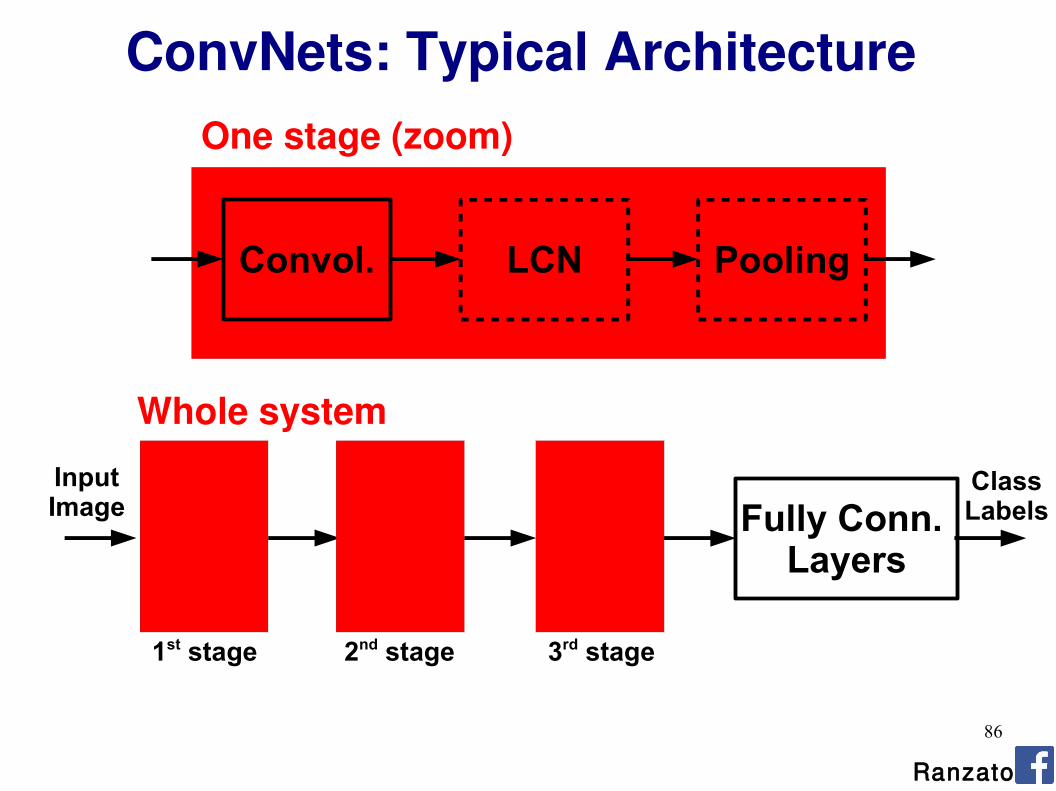
Note: after one stage the number of feature maps is usually increased (conv. layer) and the spatial resolution is usually decreased (stride in conv. and pooling layers). Receptive field gets bigger.
Reasons:- gain invariance to spatial translation (pooling layer)- increase specificity of features (approaching object specific units)
86
Convol. LCN Pooling
One stage (zoom)
Fully Conn. Layers
Whole system
1st stage 2nd stage 3rd stage
Input Image
ClassLabels
Ranzato
ConvNets: Typical Architecture

87
SIFT → K-Means → Pyramid Pooling → SVM
SIFT → Fisher Vect. → Pooling → SVM
Lazebnik et al. “...Spatial Pyramid Matching...” CVPR 2006
Sanchez et al. “Image classifcation with F.V.: Theory and practice” IJCV 2012
Conceptually similar to:
Ranzato
Fully Conn. Layers
Whole system
1st stage 2nd stage 3rd stage
Input Image
ClassLabels
ConvNets: Typical Architecture
88
ConvNets: Training
Algorithm:Given a small mini-batch- F-PROP- B-PROP- PARAMETER UPDATE
All layers are differentiable (a.e.). We can use standard back-propagation.
Ranzato

89
Ranzato
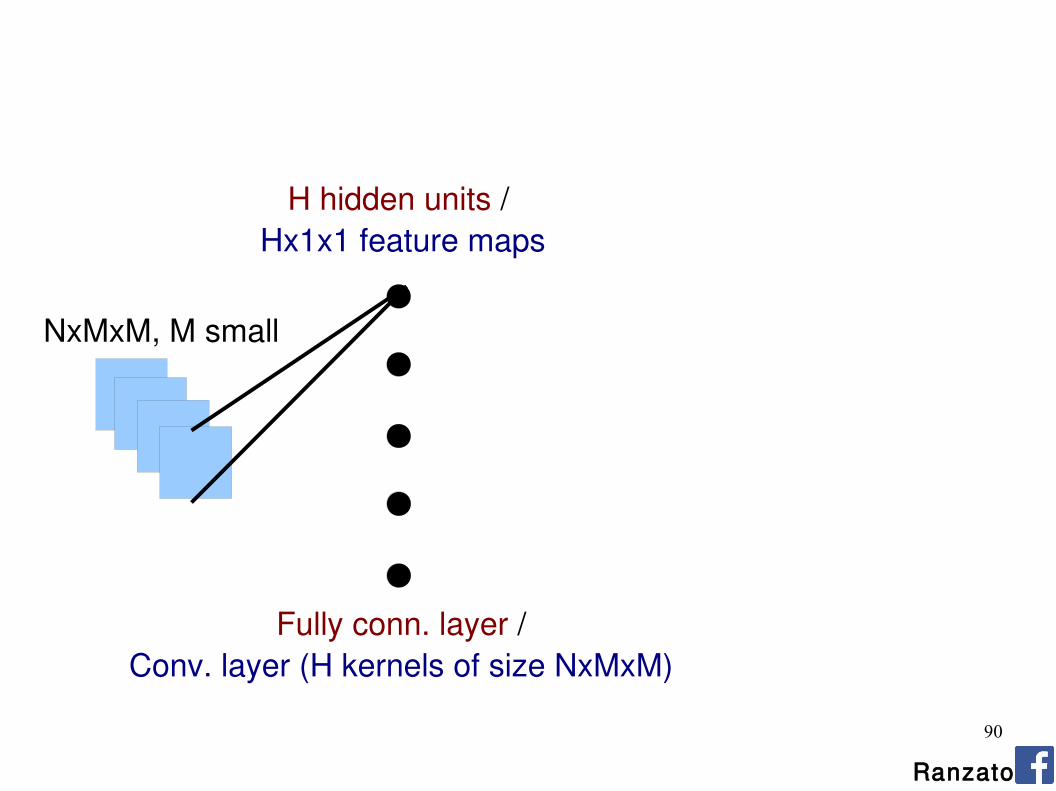
Note: After several stages of convolution-pooling, the spatial resolution is greatly reduced (usually to about 5x5) and the number of feature maps is large (several hundreds depending on the application).
It would not make sense to convolve again (there is no translation invariance and support is too small). Everything is vectorized and fed into several fully connected layers.
If the input of the fully connected layers is of size Nx5x5, the first fully connected layer can be seen as a conv. layer with 5x5 kernels.The next fully connected layer can be seen as a conv. layer with 1x1 kernels.
90
Ranzato
NxMxM, M small
H hidden units / Hx1x1 feature maps
Fully conn. layer /Conv. layer (H kernels of size NxMxM)

91
NxMxM, M small
H hidden units / Hx1x1 feature maps
Fully conn. layer /Conv. layer (H kernels of size NxMxM)
K hidden units / Kx1x1 feature maps
Fully conn. layer /Conv. layer (K kernels of size Hx1x1)

92
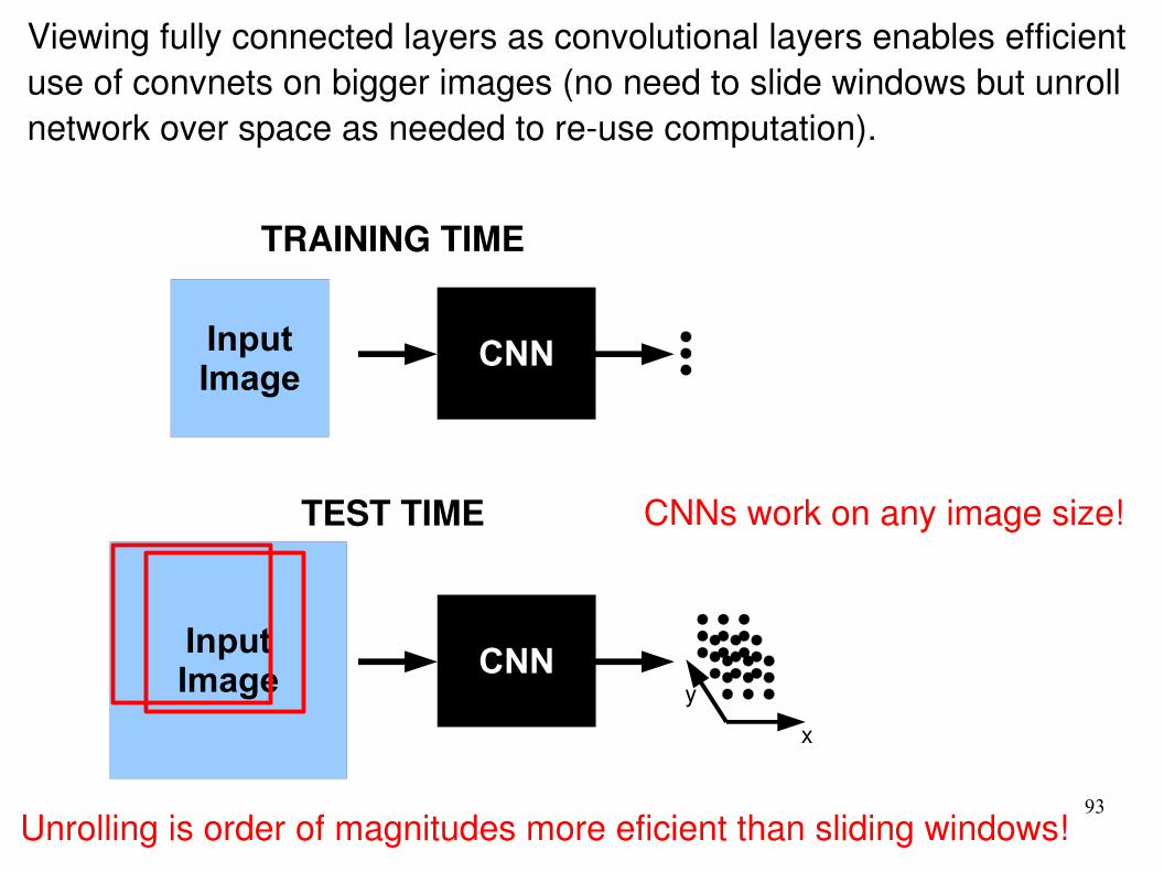
Viewing fully connected layers as convolutional layers enables efficient use of convnets on bigger images (no need to slide windows but unroll network over space as needed to re-use computation).
CNNInputImage
CNNInputImageInputImage
TRAINING TIME
TEST TIME
x
y
93
Viewing fully connected layers as convolutional layers enables efficient use of convnets on bigger images (no need to slide windows but unroll network over space as needed to re-use computation).
CNNInputImage
CNNInputImage
TRAINING TIME
TEST TIME
x
y
Unrolling is order of magnitudes more eficient than sliding windows!
CNNs work on any image size!
94
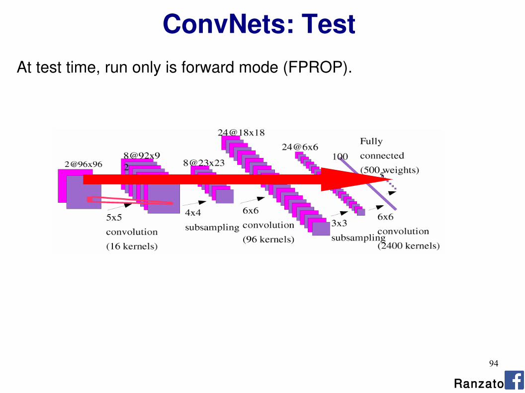
ConvNets: TestAt test time, run only is forward mode (FPROP).
Ranzato
95
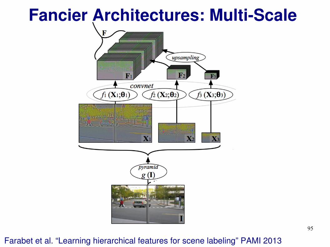
Fancier Architectures: Multi-Scale
Farabet et al. “Learning hierarchical features for scene labeling” PAMI 2013
96
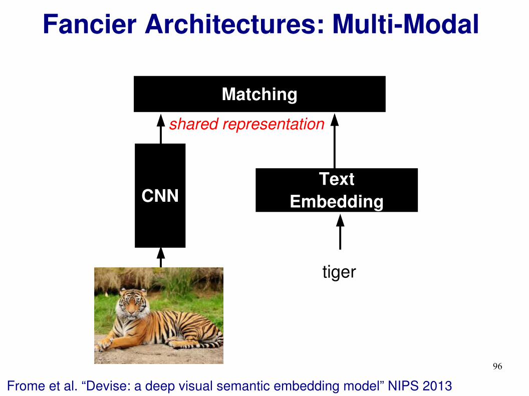
Fancier Architectures: Multi-Modal
Frome et al. “Devise: a deep visual semantic embedding model” NIPS 2013
CNNText
Embedding
tiger
Matching
shared representation

97
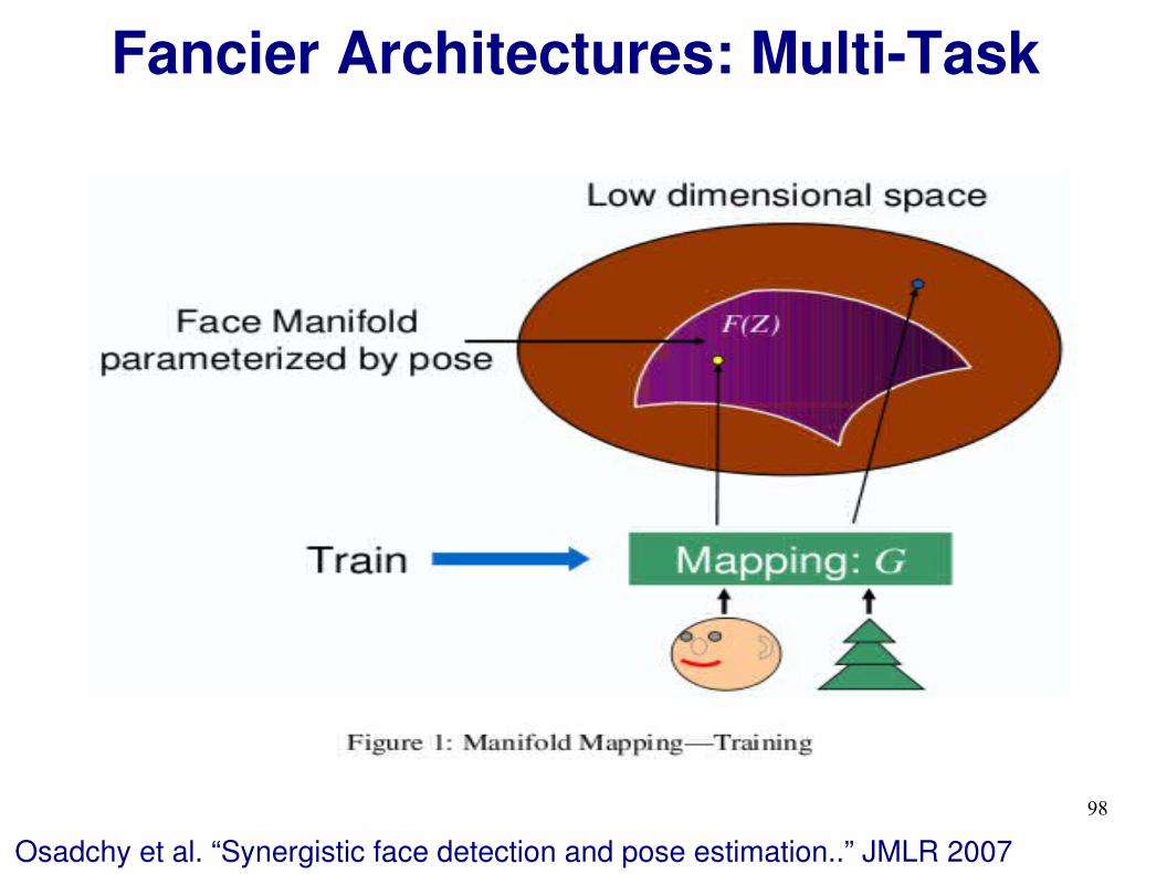
Fancier Architectures: Multi-Task
Zhang et al. “PANDA..” CVPR 2014
ConvNormPool
ConvNormPool
ConvNormPool
ConvNormPool
FullyConn.
FullyConn.
FullyConn.
FullyConn.
...
Attr. 1
Attr. 2
Attr. N
image
98
Fancier Architectures: Multi-Task
Osadchy et al. “Synergistic face detection and pose estimation..” JMLR 2007

99
Fancier Architectures: Generic DAG
Any DAG of differentialble modules is allowed!

100
Fancier Architectures: Generic DAGIf there are cycles (RNN), one needs to un-roll it.
Graves “Offline Arabic handwriting recognition..” Springer 2012

101
Outline
Ranzato
Supervised Neural Networks
Convolutional Neural Networks
Examples
Tips
102
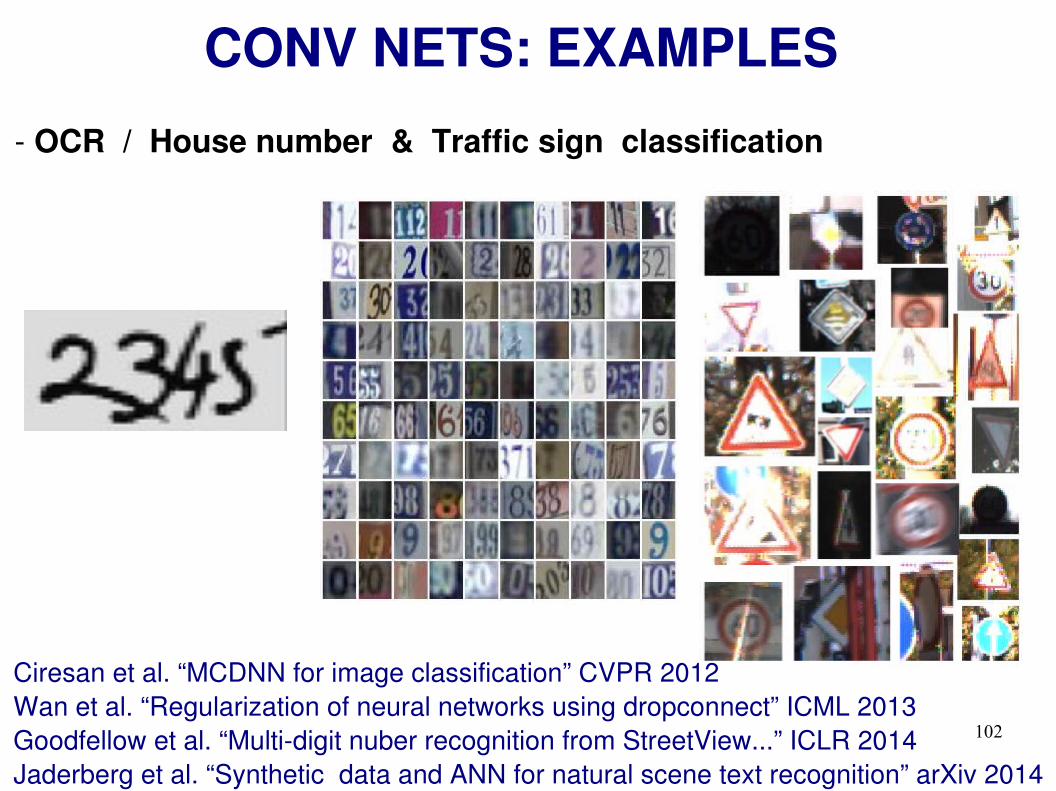
CONV NETS: EXAMPLES- OCR / House number & Traffic sign classification
Ciresan et al. “MCDNN for image classification” CVPR 2012Wan et al. “Regularization of neural networks using dropconnect” ICML 2013Goodfellow et al. “Multi-digit nuber recognition from StreetView...” ICLR 2014Jaderberg et al. “Synthetic data and ANN for natural scene text recognition” arXiv 2014
103
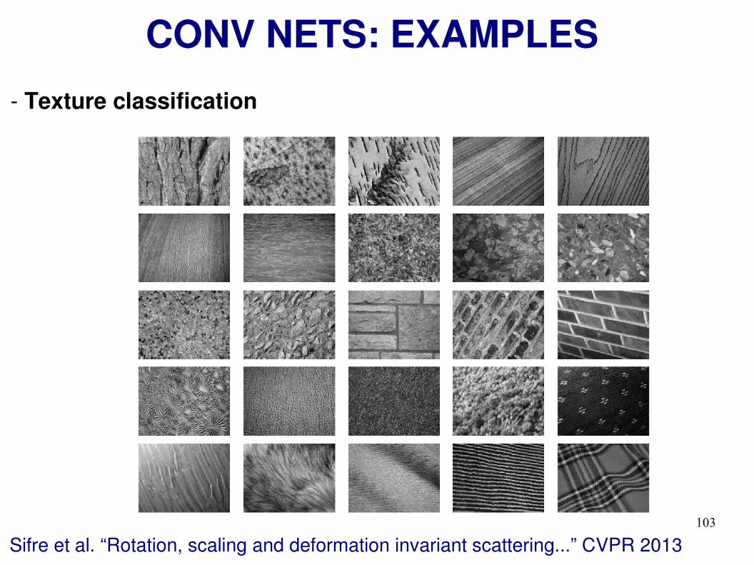
CONV NETS: EXAMPLES- Texture classification
Sifre et al. “Rotation, scaling and deformation invariant scattering...” CVPR 2013
104
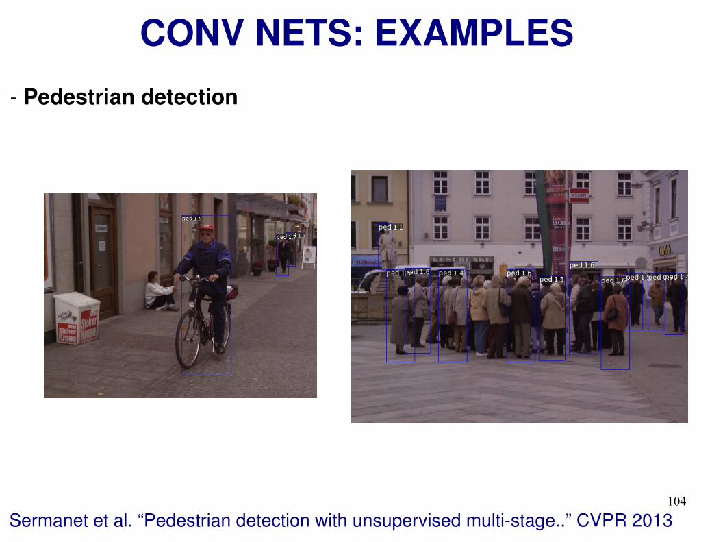
CONV NETS: EXAMPLES- Pedestrian detection
Sermanet et al. “Pedestrian detection with unsupervised multi-stage..” CVPR 2013

105
CONV NETS: EXAMPLES- Scene Parsing
Farabet et al. “Learning hierarchical features for scene labeling” PAMI 2013RanzatoPinheiro et al. “Recurrent CNN for scene parsing” arxiv 2013
106
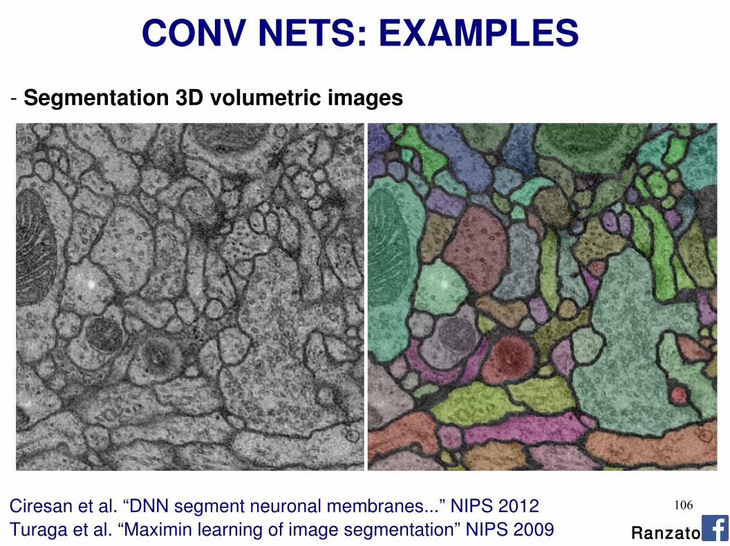
CONV NETS: EXAMPLES- Segmentation 3D volumetric images
Ciresan et al. “DNN segment neuronal membranes...” NIPS 2012Turaga et al. “Maximin learning of image segmentation” NIPS 2009 Ranzato

107
CONV NETS: EXAMPLES- Action recognition from videos
Taylor et al. “Convolutional learning of spatio-temporal features” ECCV 2010Karpathy et al. “Large-scale video classification with CNNs” CVPR 2014Simonyan et al. “Two-stream CNNs for action recognition in videos” arXiv 2014
108
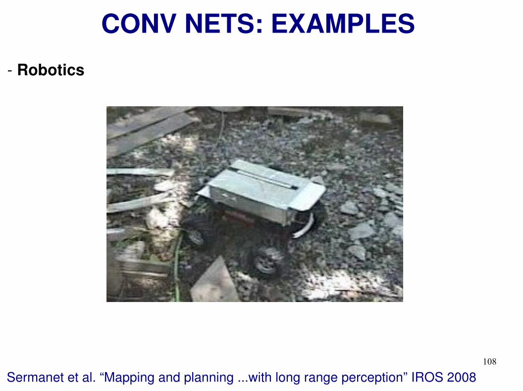
CONV NETS: EXAMPLES- Robotics
Sermanet et al. “Mapping and planning ...with long range perception” IROS 2008
109
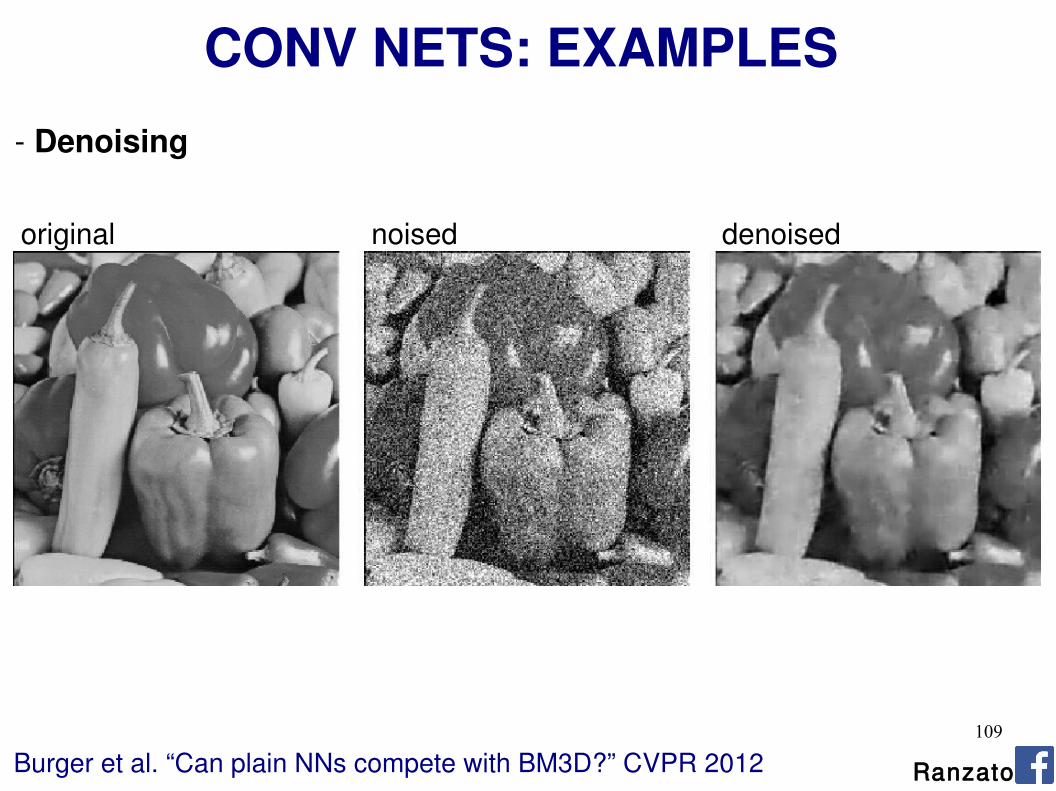
CONV NETS: EXAMPLES- Denoising
Burger et al. “Can plain NNs compete with BM3D?” CVPR 2012
original noised denoised
Ranzato
110
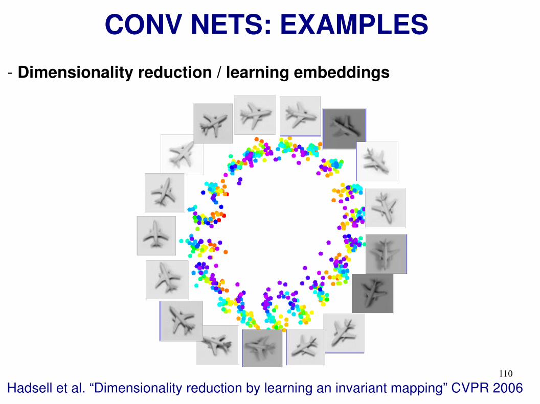
CONV NETS: EXAMPLES- Dimensionality reduction / learning embeddings
Hadsell et al. “Dimensionality reduction by learning an invariant mapping” CVPR 2006
111
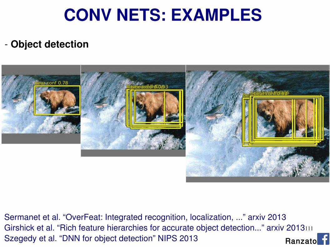
CONV NETS: EXAMPLES- Object detection
Sermanet et al. “OverFeat: Integrated recognition, localization, ...” arxiv 2013
Szegedy et al. “DNN for object detection” NIPS 2013 RanzatoGirshick et al. “Rich feature hierarchies for accurate object detection...” arxiv 2013
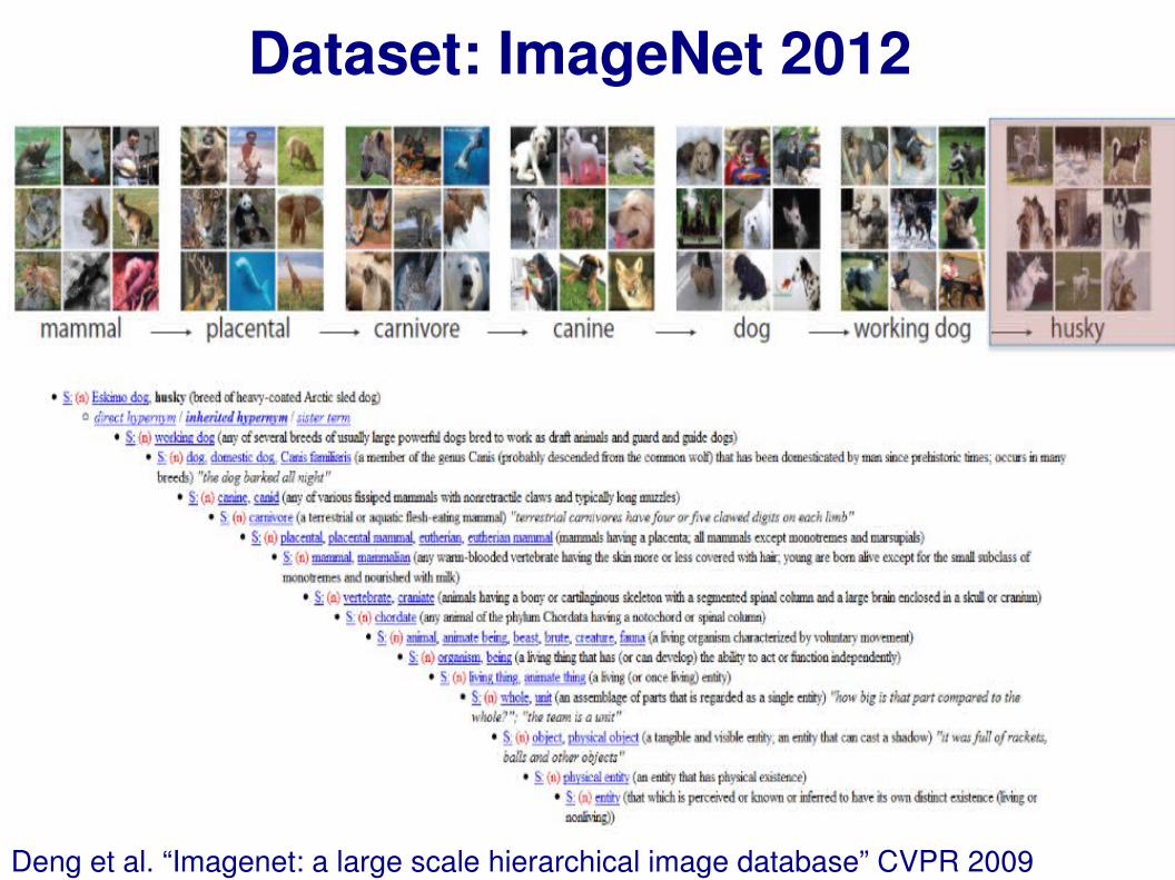
Dataset: ImageNet 2012
Deng et al. “Imagenet: a large scale hierarchical image database” CVPR 2009

ImageNetExamples of hammer:
114
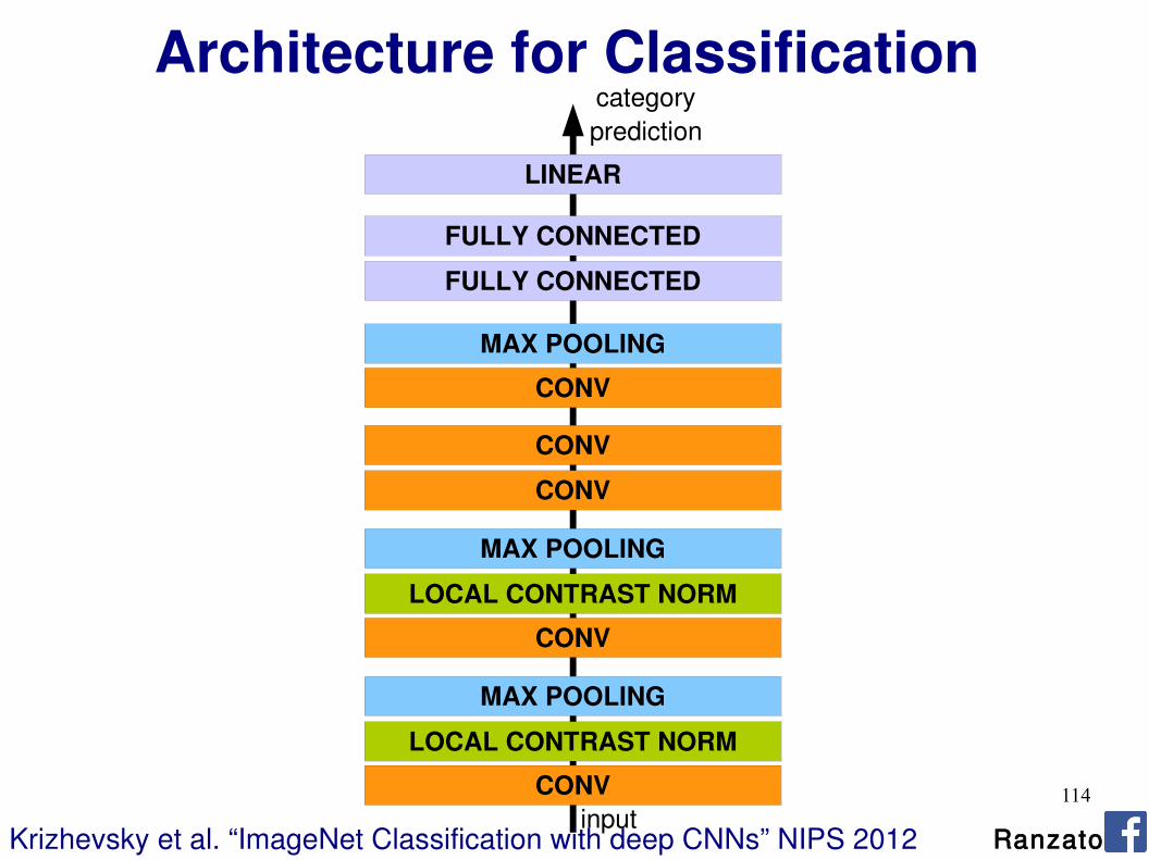
Architecture for Classification
CONV
LOCAL CONTRAST NORM
MAX POOLING
FULLY CONNECTED
LINEAR
CONV
LOCAL CONTRAST NORM
MAX POOLING
CONV
CONV
CONV
MAX POOLING
FULLY CONNECTED
Krizhevsky et al. “ImageNet Classification with deep CNNs” NIPS 2012
category prediction
input Ranzato

115CONV
LOCAL CONTRAST NORM
MAX POOLING
FULLY CONNECTED
LINEAR
CONV
LOCAL CONTRAST NORM
MAX POOLING
CONV
CONV
CONV
MAX POOLING
FULLY CONNECTED
Total nr. params: 60M4M
16M
37M
442K
1.3M
884K
307K
35K
Total nr. flops: 832M4M
16M37M
74M
224M
149M
223M
105M
Krizhevsky et al. “ImageNet Classification with deep CNNs” NIPS 2012
category prediction
input Ranzato
Architecture for Classification

116
Optimization
SGD with momentum:
Learning rate = 0.01
Momentum = 0.9
Improving generalization by:
Weight sharing (convolution)
Input distortions
Dropout = 0.5
Weight decay = 0.0005
Ranzato

117
Results: ILSVRC 2012
RanzatoKrizhevsky et al. “ImageNet Classification with deep CNNs” NIPS 2012

118
119
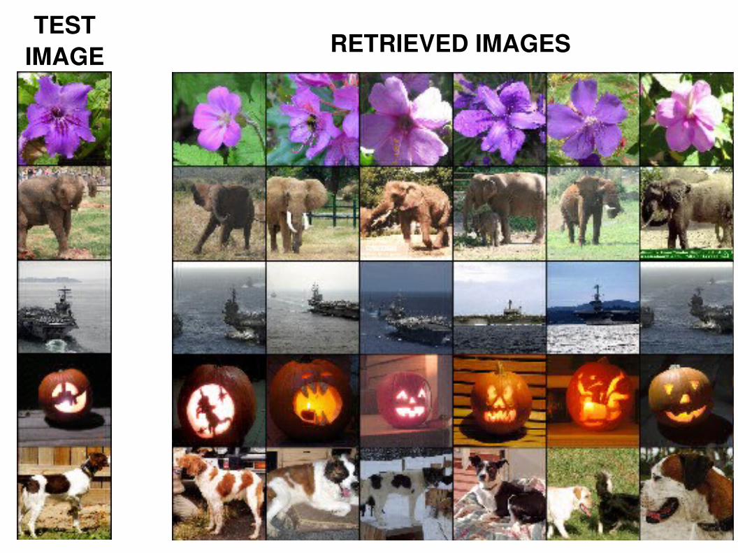
TEST IMAGE RETRIEVED IMAGES
120
Outline
Ranzato
Supervised Neural Networks
Convolutional Neural Networks
Examples
Tips
121
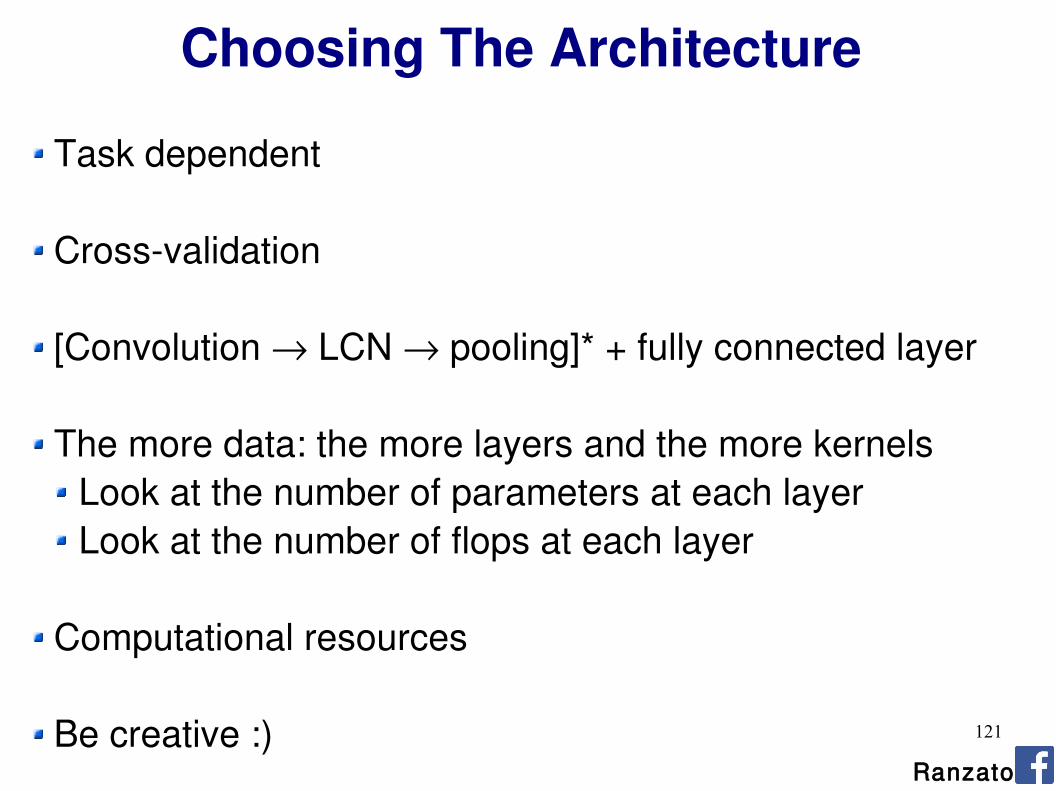
Choosing The Architecture
Task dependent
Cross-validation
[Convolution → LCN → pooling]* + fully connected layer
The more data: the more layers and the more kernelsLook at the number of parameters at each layerLook at the number of flops at each layer
Computational resources
Be creative :)Ranzato

122
How To Optimize
SGD (with momentum) usually works very well
Pick learning rate by running on a subset of the dataBottou “Stochastic Gradient Tricks” Neural Networks 2012Start with large learning rate and divide by 2 until loss does not divergeDecay learning rate by a factor of ~1000 or more by the end of training
Use non-linearity
Initialize parameters so that each feature across layers has similar variance. Avoid units in saturation.
Ranzato

123
Improving Generalization
Weight sharing (greatly reduce the number of parameters)
Data augmentation (e.g., jittering, noise injection, etc.)
Dropout Hinton et al. “Improving Nns by preventing co-adaptation of feature detectors” arxiv 2012
Weight decay (L2, L1)
Sparsity in the hidden units
Multi-task (unsupervised learning)
Ranzato
124
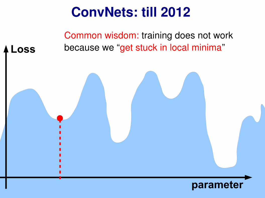
ConvNets: till 2012
Loss
parameter
Common wisdom: training does not work because we “get stuck in local minima”

125
ConvNets: today
Loss
parameter
Local minima are all similar, there are long plateaus, it can take long time to break symmetries.
w w
input/output invariant to permutationsbreaking ties
between parameters
W T X
1
Saturating units
Dauphin et al. “Identifying and attacking the saddle point problem..” arXiv 2014
126
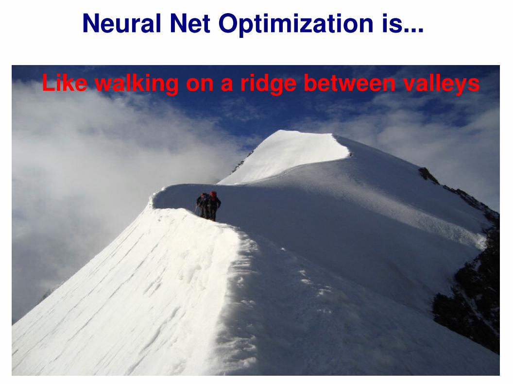
Like walking on a ridge between valleys
Neural Net Optimization is...
127
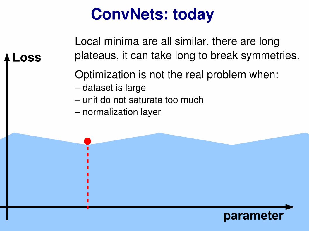
ConvNets: today
Loss
parameter
Local minima are all similar, there are long plateaus, it can take long to break symmetries.
Optimization is not the real problem when:– dataset is large– unit do not saturate too much– normalization layer
128
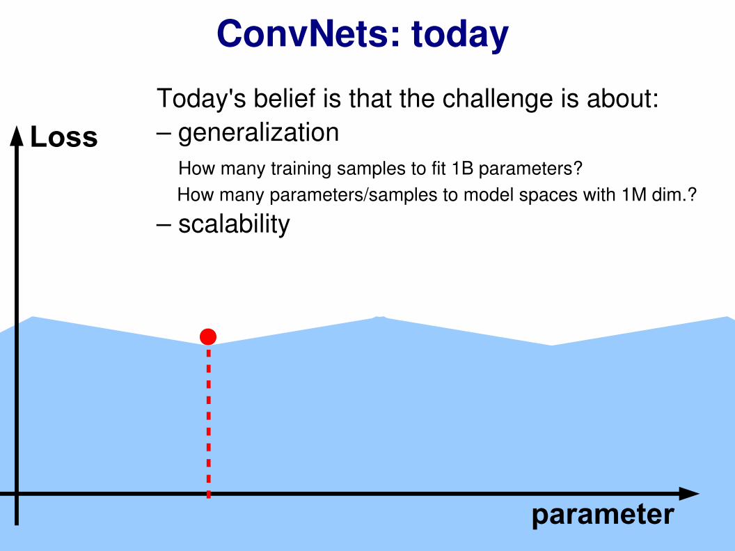
ConvNets: today
Loss
parameter
Today's belief is that the challenge is about:– generalization How many training samples to fit 1B parameters? How many parameters/samples to model spaces with 1M dim.?
– scalability

129
data
flops/s
capacity
T IME
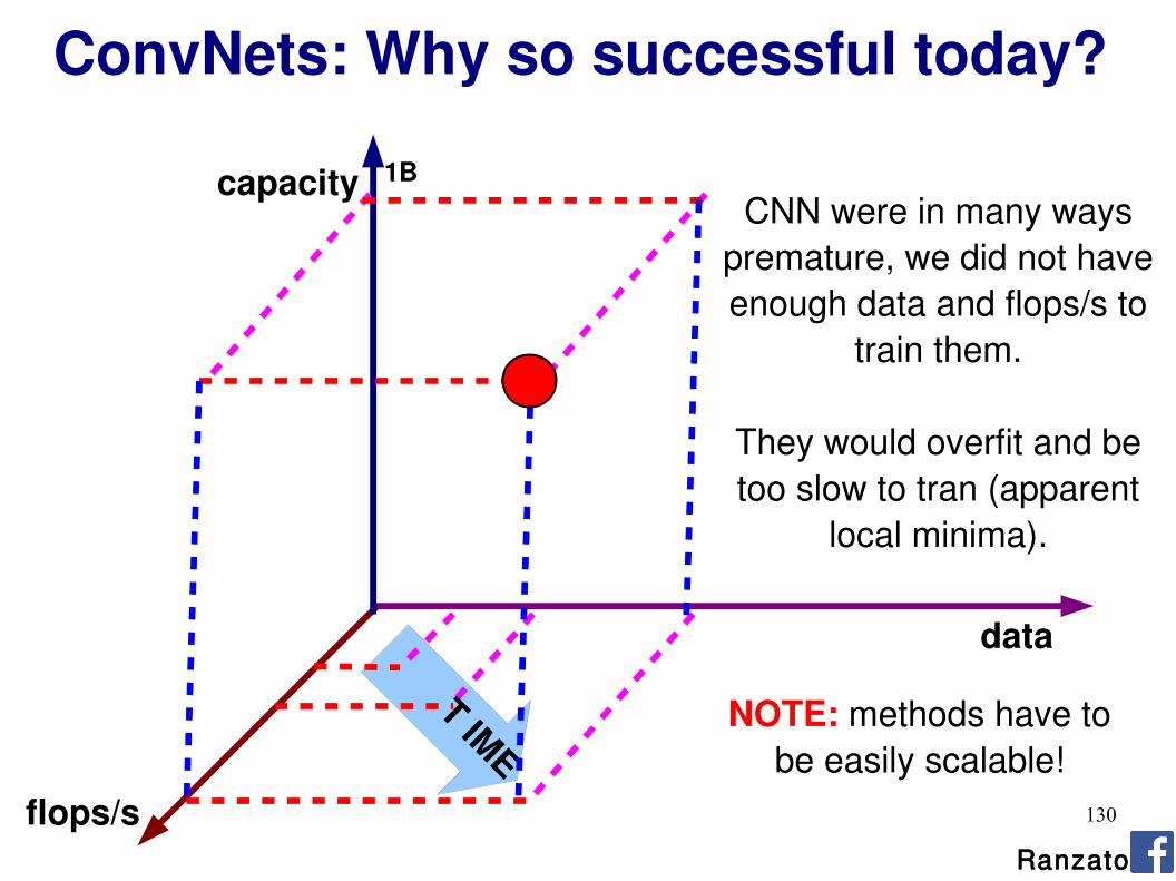
ConvNets: Why so successful today?
T IM
E
As time goes by, we get more data and more flops/s. The capacity of ML models should grow
accordingly.
1K 1M 1B
1M
100M
10T
Ranzato
130
data
capacity
T IME
ConvNets: Why so successful today?
CNN were in many ways premature, we did not have enough data and flops/s to
train them.
They would overfit and be too slow to tran (apparent
local minima).
flops/s
1B
NOTE: methods have to be easily scalable!
Ranzato
131
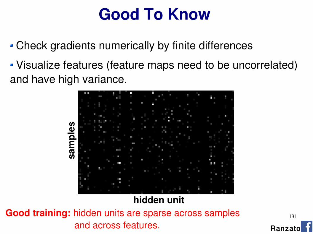
Good To Know
Check gradients numerically by finite differences
Visualize features (feature maps need to be uncorrelated) and have high variance.
sam
p les
hidden unitGood training: hidden units are sparse across samples and across features. Ranzato

132
Check gradients numerically by finite differences
Visualize features (feature maps need to be uncorrelated) and have high variance.
sam
p les
hidden unitBad training: many hidden units ignore the input and/or exhibit strong correlations. Ranzato
Good To Know
133
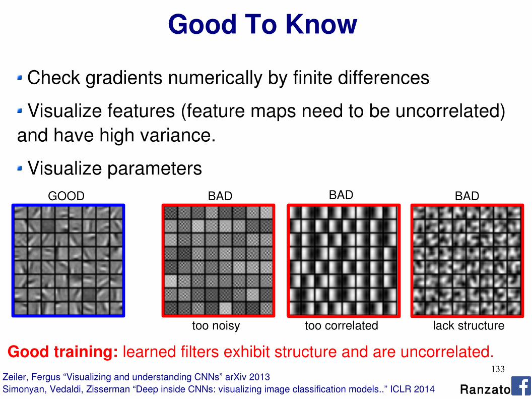
Check gradients numerically by finite differences
Visualize features (feature maps need to be uncorrelated) and have high variance.
Visualize parameters
Good training: learned filters exhibit structure and are uncorrelated.
GOOD BADBAD BAD
too noisy too correlated lack structure
Ranzato
Good To Know
Zeiler, Fergus “Visualizing and understanding CNNs” arXiv 2013Simonyan, Vedaldi, Zisserman “Deep inside CNNs: visualizing image classification models..” ICLR 2014

134
Check gradients numerically by finite differences
Visualize features (feature maps need to be uncorrelated) and have high variance.
Visualize parameters
Measure error on both training and validation set.
Test on a small subset of the data and check the error → 0.
Ranzato
Good To Know
135
What If It Does Not Work?
Training diverges:Learning rate may be too large → decrease learning rateBPROP is buggy → numerical gradient checking
Parameters collapse / loss is minimized but accuracy is low Check loss function:
Is it appropriate for the task you want to solve?Does it have degenerate solutions? Check “pull-up” term.
Network is underperformingCompute flops and nr. params. → if too small, make net largerVisualize hidden units/params → fix optmization
Network is too slowCompute flops and nr. params. → GPU,distrib. framework, make net smaller
Ranzato
136
Summary Part I Deep Learning = learning hierarhical models. ConvNets are the
most successful example. Leverage large labeled datasets.
OptimizationDon't we get stuck in local minima? No, they are all the same!In large scale applications, local minima are even less of an issue.
ScalingGPUsDistributed framework (Google)Better optimization techniques
Generalization on small datasets (curse of dimensionality): data augmentation weight decay dropout unsupervised learning multi-task learning
Ranzato
137
SOFTWARETorch7: learning library that supports neural net traininghttp://www.torch.chhttp://code.cogbits.com/wiki/doku.php (tutorial with demos by C. Farabet)https://github.com/sermanet/OverFeat
Python-based learning library (U. Montreal)
- http://deeplearning.net/software/theano/ (does automatic differentiation)
Caffe (Yangqing Jia)
– http://caffe.berkeleyvision.org
Efficient CUDA kernels for ConvNets (Krizhevsky)
– code.google.com/p/cuda-convnet
Ranzato
138
REFERENCESConvolutional Nets– LeCun, Bottou, Bengio and Haffner: Gradient-Based Learning Applied to Document Recognition, Proceedings of the IEEE, 86(11):2278-2324, November 1998
- Krizhevsky, Sutskever, Hinton “ImageNet Classification with deep convolutional neural networks” NIPS 2012
– Jarrett, Kavukcuoglu, Ranzato, LeCun: What is the Best Multi-Stage Architecture for Object Recognition?, Proc. International Conference on Computer Vision (ICCV'09), IEEE, 2009
- Kavukcuoglu, Sermanet, Boureau, Gregor, Mathieu, LeCun: Learning Convolutional Feature Hierachies for Visual Recognition, Advances in Neural Information Processing Systems (NIPS 2010), 23, 2010
– see yann.lecun.com/exdb/publis for references on many different kinds of convnets.
– see http://www.cmap.polytechnique.fr/scattering/ for scattering networks (similar to convnets but with less learning and stronger mathematical foundations)
– see http://www.idsia.ch/~juergen/ for other references to ConvNets and LSTMs.Ranzato
139
REFERENCESApplications of Convolutional Nets
– Farabet, Couprie, Najman, LeCun. Scene Parsing with Multiscale Feature Learning, Purity Trees, and Optimal Covers”, ICML 2012
– Pierre Sermanet, Koray Kavukcuoglu, Soumith Chintala and Yann LeCun: Pedestrian Detection with Unsupervised Multi-Stage Feature Learning, CVPR 2013
- D. Ciresan, A. Giusti, L. Gambardella, J. Schmidhuber. Deep Neural Networks Segment Neuronal Membranes in Electron Microscopy Images. NIPS 2012
- Raia Hadsell, Pierre Sermanet, Marco Scoffier, Ayse Erkan, Koray Kavackuoglu, Urs Muller and Yann LeCun. Learning Long-Range Vision for Autonomous Off-Road Driving, Journal of Field Robotics, 26(2):120-144, 2009
– Burger, Schuler, Harmeling. Image Denoisng: Can Plain Neural Networks Compete with BM3D?, CVPR 2012
– Hadsell, Chopra, LeCun. Dimensionality reduction by learning an invariant mapping, CVPR 2006
– Bergstra et al. Making a science of model search: hyperparameter optimization in hundred of dimensions for vision architectures, ICML 2013 Ranzato

140
REFERENCESLatest and Greatest Convolutional Nets– Girshick, Donahue, Darrell, Malick. “Rich feature hierarchies for accurate object detection and semantic segmentation”, arXiv 2014
– Simonyan, Zisserman “Two-stream CNNs for action recognition in videos” arXiv 2014
- Cadieu, Hong, Yamins, Pinto, Ardila, Solomon, Majaj, DiCarlo. “DNN rival in representation of primate IT cortex for core visual object recognition”. arXiv 2014
- Erhan, Szegedy, Toshev, Anguelov “Scalable object detection using DNN” CVPR 2014
- Razavian, Azizpour, Sullivan, Carlsson “CNN features off-the-shelf: and astounding baseline for recognition” arXiv 2014
- Krizhevsky “One weird trick for parallelizing CNNs” arXiv 2014
Ranzato
141
REFERENCESDeep Learning in general
– deep learning tutorial @ CVPR 2014 https://sites.google.com/site/deeplearningcvpr2014/
– deep learning tutorial slides at ICML 2013: icml.cc/2013/?page_id=39
– Yoshua Bengio, Learning Deep Architectures for AI, Foundations and Trends in Machine Learning, 2(1), pp.1-127, 2009.
– LeCun, Chopra, Hadsell, Ranzato, Huang: A Tutorial on Energy-Based Learning, in Bakir, G. and Hofman, T. and Schölkopf, B. and Smola, A. and Taskar, B. (Eds), Predicting Structured Data, MIT Press, 2006
Ranzato
“Theory” of Deep Learning
– Mallat: Group Invariant Scattering, Comm. In Pure and Applied Math. 2012
– Pascanu, Montufar, Bengio: On the number of inference regions of DNNs with piece wise linear activations, ICLR 2014
– Pascanu, Dauphin, Ganguli, Bengio: On the saddle-point problem for non-convex optimization, arXiv 2014
- Delalleau, Bengio: Shallow vs deep Sum-Product Networks, NIPS 2011

142
THE END - PART I
Ranzato
143
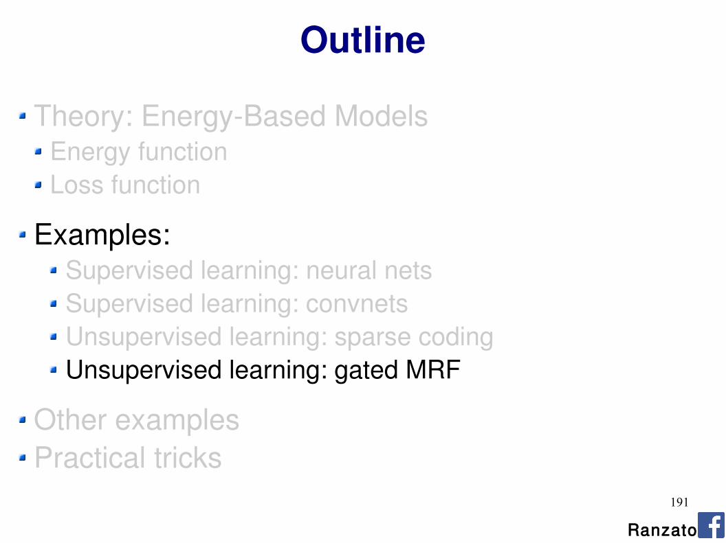
Outline Part II
Theory: Energy-Based ModelsEnergy functionLoss function
Examples:Supervised learning: neural netsUnsupervised learning: sparse codingUnsupervised learning: gated MRF
Conclusions
Ranzato
144
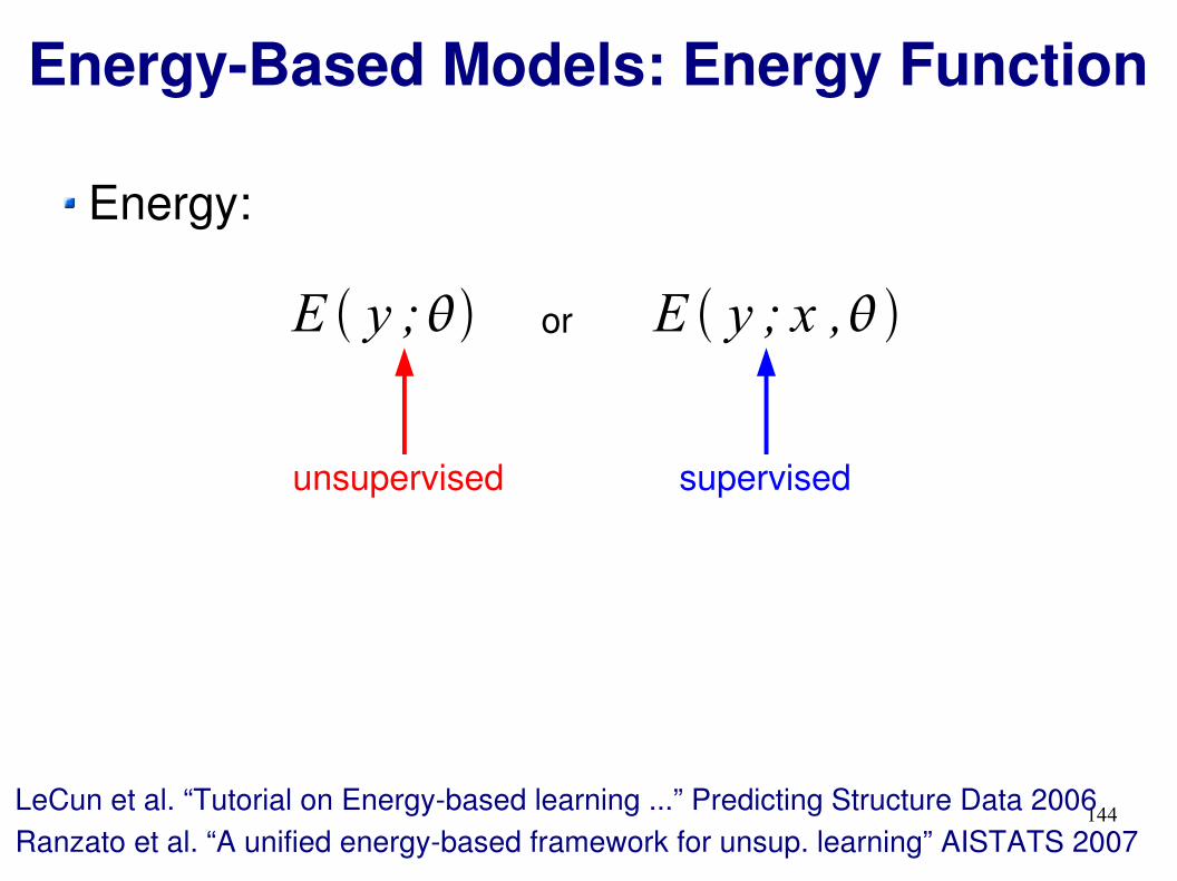
Energy:
LeCun et al. “Tutorial on Energy-based learning ...” Predicting Structure Data 2006Ranzato et al. “A unified energy-based framework for unsup. learning” AISTATS 2007
Energy-Based Models: Energy Function
E y ; E y ; x ,or
unsupervised supervised
145
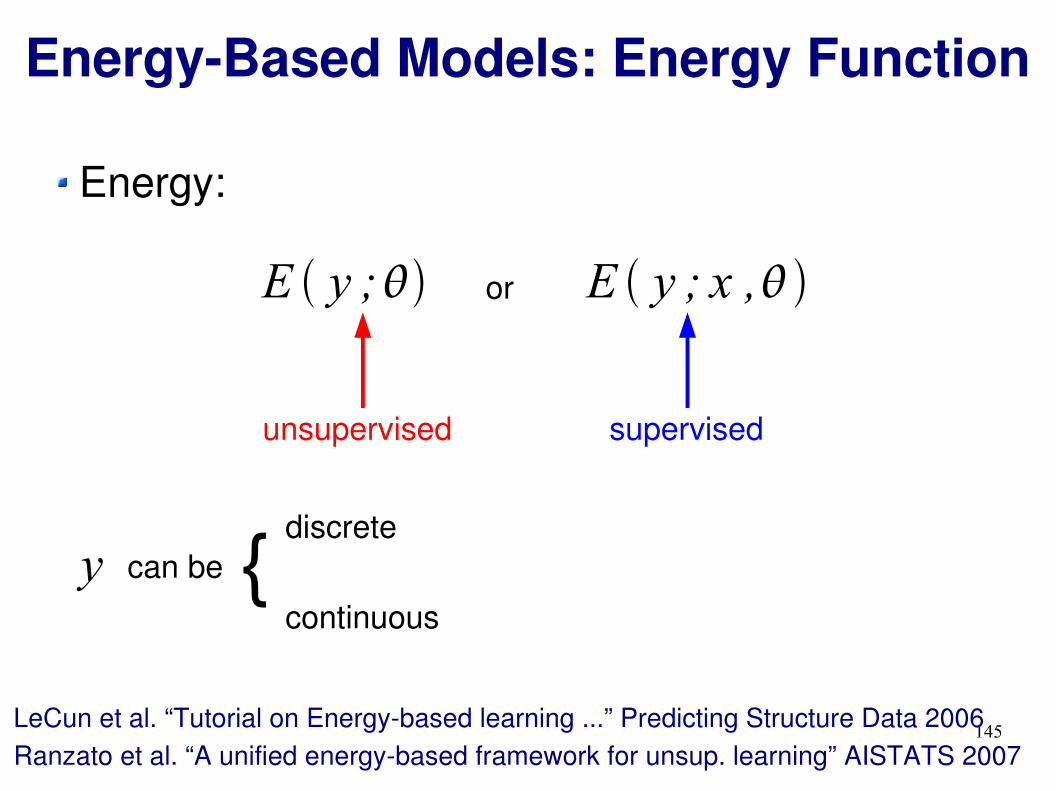
Energy:
LeCun et al. “Tutorial on Energy-based learning ...” Predicting Structure Data 2006Ranzato et al. “A unified energy-based framework for unsup. learning” AISTATS 2007
Energy-Based Models: Energy Function
E y ; E y ; x ,or
unsupervised supervised
y can be discrete
continuous{
146
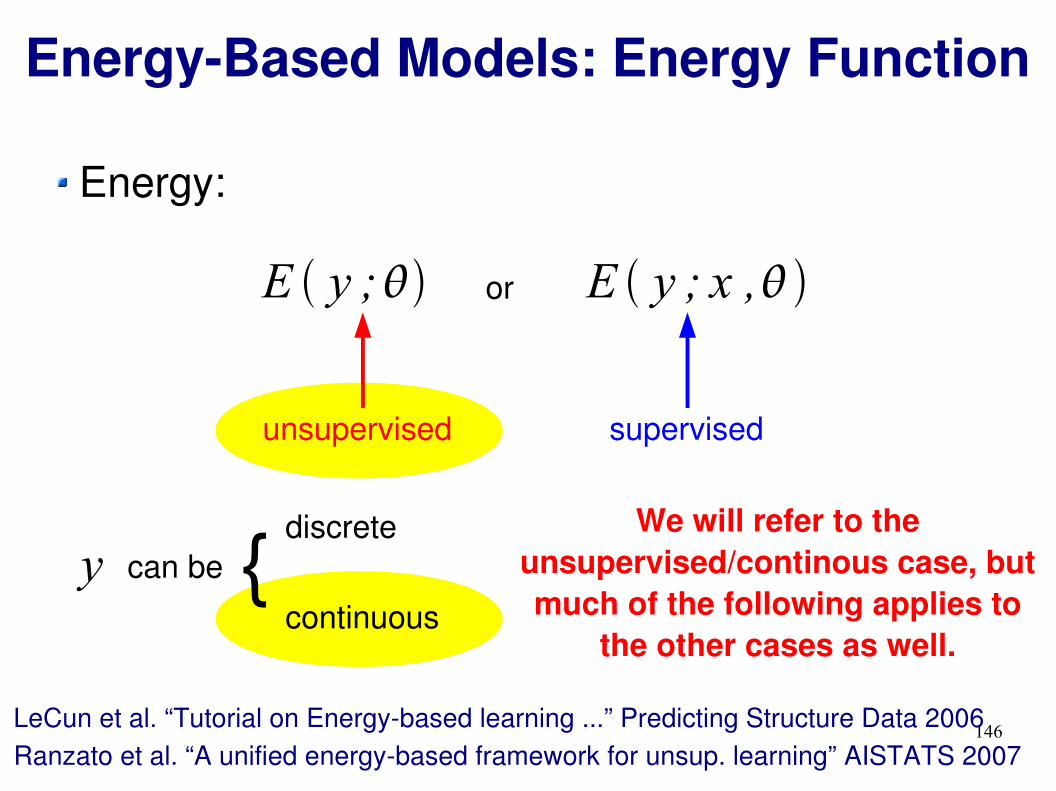
Energy:
LeCun et al. “Tutorial on Energy-based learning ...” Predicting Structure Data 2006Ranzato et al. “A unified energy-based framework for unsup. learning” AISTATS 2007
Energy-Based Models: Energy Function
E y ; E y ; x ,or
unsupervised supervised
y can be discrete
continuous{
We will refer to the unsupervised/continous case, but much of the following applies to
the other cases as well.

147
Energy should be lower for desired output
E
y
Energy-Based Models: Energy Function
Ranzato

148
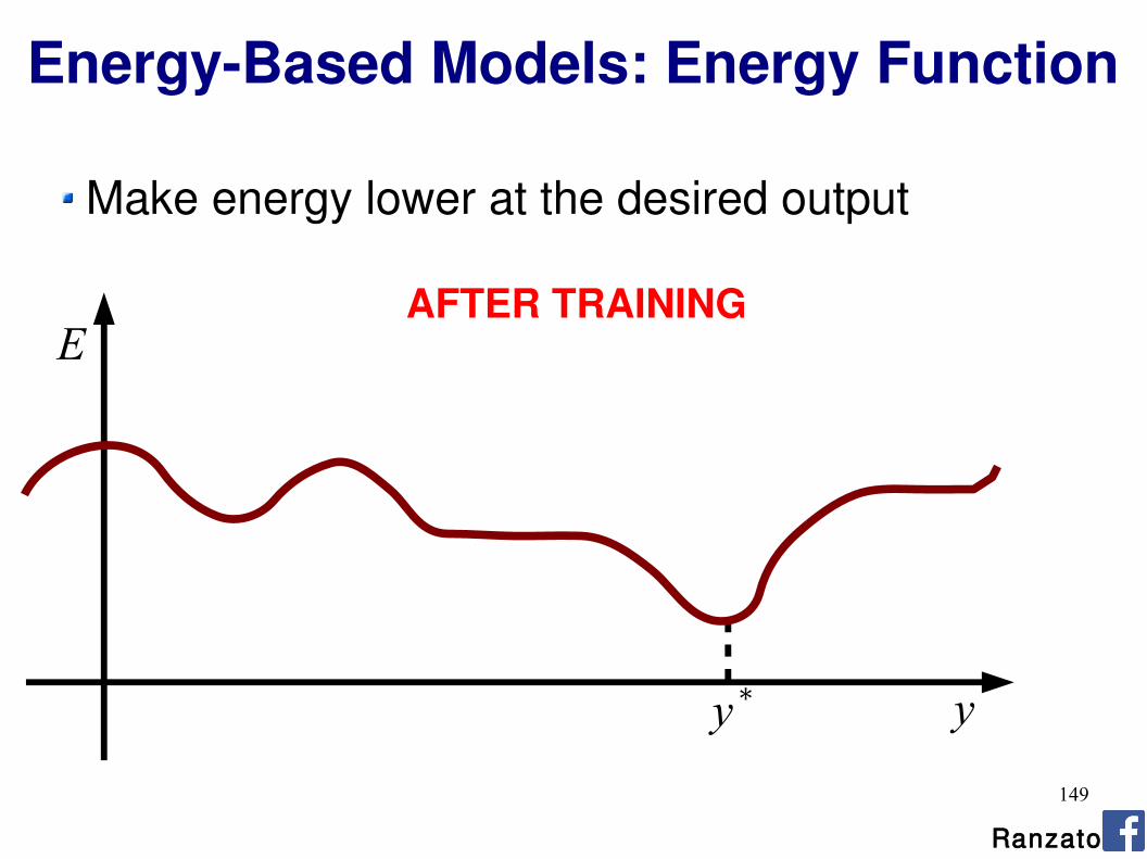
Make energy lower at the desired output
E
yy∗
BEFORE TRAINING
Energy-Based Models: Energy Function
Ranzato
149
Make energy lower at the desired output
E
yy∗
AFTER TRAINING
Energy-Based Models: Energy Function
Ranzato

150
Examples of energy function:
PCA
Linear binary classifier
Neural net binary classifier
Energy-Based Models: Energy Function
E y=∥y−W W T y∥22
E y ; x =− y W T x
y∈{−1,1}
E y ; x =− y W 2T f x ;W 1

151
Energy-Based Models: Loss Function
Loss is a function of the energy
Minimizing the loss over the training set yields the desired energy landscape.
∗=min∑ p
L E y p ;
Examples of loss function:PCA
Logistic regression classifier
E y=∥y−W W T y∥22
E y ; x =− y W T x
L E y=E y
L E y ; x =log 1exp E y ; x

152
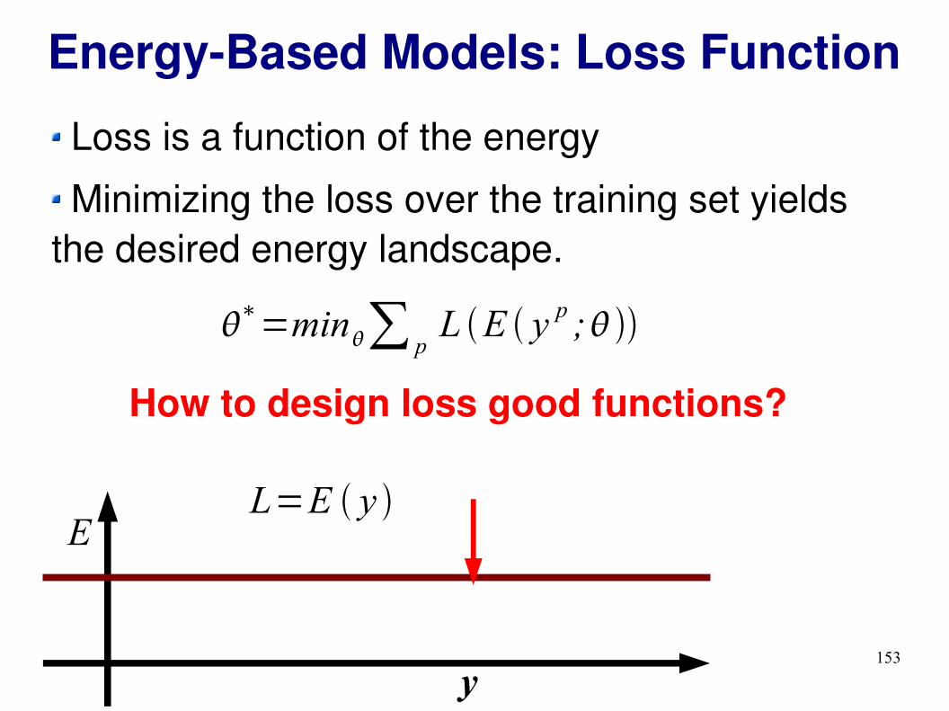
Energy-Based Models: Loss Function
Loss is a function of the energy
Minimizing the loss over the training set yields the desired energy landscape.
∗=min∑ p
L E y p ;
How to design loss good functions?
Ranzato
153
Energy-Based Models: Loss Function
Loss is a function of the energy
Minimizing the loss over the training set yields the desired energy landscape.
∗=min∑ p
L E y p ;
E
y
L=E y
How to design loss good functions?

154
Energy-Based Models: Loss Function
Loss is a function of the energy
Minimizing the loss over the training set yields the desired energy landscape.
∗=min∑ p
L E y p ;
E
y
L=E y
How to design loss good functions?

155
Energy-Based Models: Loss Function
Loss is a function of the energy
Minimizing the loss over the training set yields the desired energy landscape.
∗=min∑ p
L E y p ;
E
y
L=E y
BAD LOSS
How to design loss good functions?
Energy is degenerate:low everywhere!
156
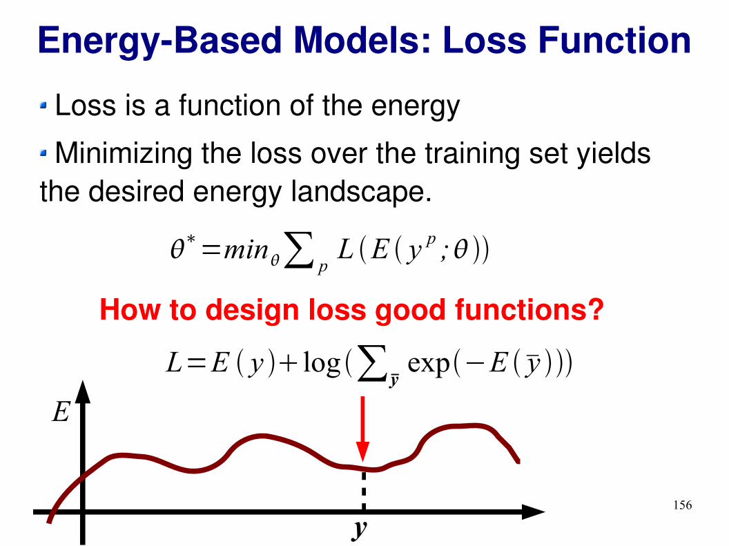
Energy-Based Models: Loss Function
Loss is a function of the energy
Minimizing the loss over the training set yields the desired energy landscape.
∗=min∑ p
L E y p ;
How to design loss good functions?
L=E y log ∑yexp−E y
E
y
157
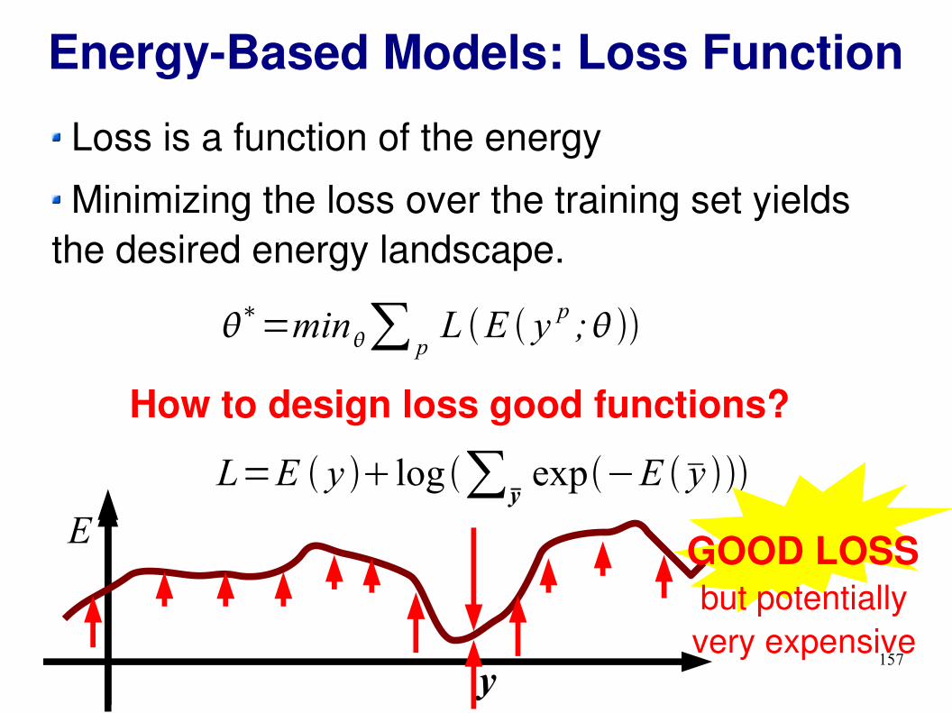
Energy-Based Models: Loss Function
Loss is a function of the energy
Minimizing the loss over the training set yields the desired energy landscape.
∗=min∑ p
L E y p ;
How to design loss good functions?
L=E y log ∑yexp−E y
E
y
GOOD LOSSbut potentially very expensive
158
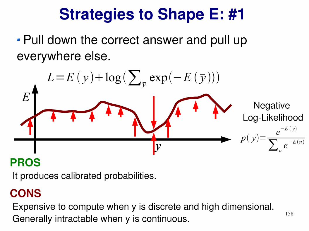
Strategies to Shape E: #1 Pull down the correct answer and pull up everywhere else.
E
y
L=E y log ∑yexp−E y
PROS It produces calibrated probabilities.
CONS Expensive to compute when y is discrete and high dimensional. Generally intractable when y is continuous.
Negative Log-Likelihood
p y=e−E y
∑ue−E u

159
Strategies to Shape E: #2 Pull down the correct answer and pull up carefully chosen points.
L=max0,m−E y −E y , e.g. y=min y≠ yE y
E
yy
E.g.: Contrastive Divergence, Ratio Matching, Noise Contrastive Estimation, Minimum Probability Flow...
Hinton et al. “A fast learning algorithm for DBNs” Neural Comp. 2008
Gutmann et al. “Noise contrastive estimation of unnormalized...” JMLR 2012Hyvarinen “Some extensions of score matchine” Comp Stats 2007
Sohl-Dickstein et al. “Minimum probability flow learning” ICML 2011

160
Strategies to Shape E: #2 Pull down the correct answer and pull up carefully chosen points.
PROS Efficient.
CONS The criterion to pick where to pull up is tricky (overall in high dimensional spaces): trades-off computational and statistical efficiency.
L=max0,m−E y −E y , e.g. y=min y≠ yE y
E
yy
161
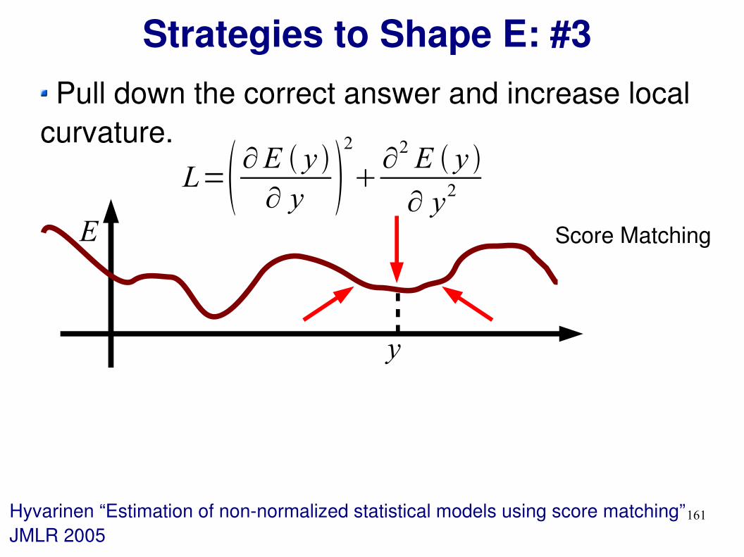
Strategies to Shape E: #3 Pull down the correct answer and increase local curvature.
E
y
Score Matching
L= ∂E y ∂ y 2
∂2 E y
∂ y2
Hyvarinen “Estimation of non-normalized statistical models using score matching” JMLR 2005
162
Strategies to Shape E: #3 Pull down the correct answer and increase local curvature.
E Score Matching
y
Hyvarinen “Estimation of non-normalized statistical models using score matching” JMLR 2005
L= ∂E y ∂ y 2
∂2 E y
∂ y2

163
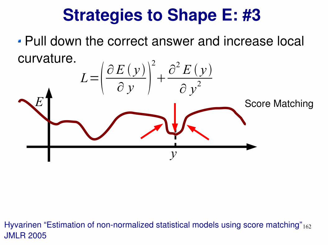
Strategies to Shape E: #3 Pull down the correct answer and increase local curvature.
PROS Efficient in continuous but not too high dimensional spaces.
CONS Very complicated to compute and not practical in very high dimensional spaces. Not applicable in discrete spaces.
E Score Matching
y
L= ∂E y ∂ y 2
∂2 E y
∂ y2

164
Strategies to Shape E: #4 Pull down correct answer and have global constrain on the energy: only few minima exist
E
y
PCA, ICA, sparse coding,...
PROS Efficient in continuous, high dimensional spaces.
L=E y
Ranzato et al. “A unified energy-based framework for unsup. learning” AISTATS 2007
CONS Need to design good global constraints. Used in unsup. learning only.

165
Strategies to Shape E: #4
E
y
PCA, ICA, sparse coding,...
L=E y
Pull down correct answer and have global constrain on the energy: only few minima exist
PROS Efficient in continuous, high dimensional spaces.
CONS Need to design good global constraints. Used in unsup. learning only.
Ranzato et al. “A unified energy-based framework for unsup. learning” AISTATS 2007

166
Strategies to Shape E: #4 Pull down correct answer and have global constrain on the energy: only few minima exist
Typical methods (unsup. learning):Use compact internal representation (PCA)Have finite number of internal states (K-Means)Use sparse codes (ICA, sparse coding)
Ranzato

167
INPUT SPACE: FEATURE SPACE:
f x ,h
g x ,h
hx
Ranzato
training sampleinput data point which is not a training samplefeature (code)

168
Wh
f x ,h
hxINPUT SPACE: FEATURE SPACE:
E.g. K-means: is 1-of-N.h
Since there are very few “codes” available and the energy (MSE) is minimized on the training set, the energy must be higher elsewhere.
Ranzato
169
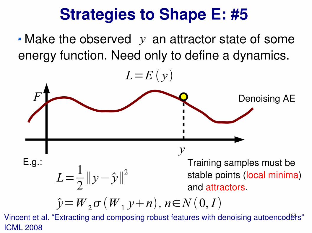
Strategies to Shape E: #5
F Denoising AE
L=E y
Make the observed an attractor state of some energy function. Need only to define a dynamics.
y
E.g.:
L=12∥y−y∥
2
y=W 2 W 1 yn , n∈N 0, I
y
Vincent et al. “Extracting and composing robust features with denoising autoencoders” ICML 2008
Training samples must be stable points (local minima)and attractors.

170
Make the observed an attractor state of some energy function. Need only to define a dynamics.
Strategies to Shape E: #5
Denoising AE
E.g.:yn
Training samples must be stable points (local minima)and attractors.
F
Kamyshanska et al. “On autoencoder scoring” ICML 2013
y
L=E y
y
y=W 2 W 1 yn , n∈N 0, I
L=12∥y−y∥
2
Ranzato

171
Make the observed an attractor state of some energy function. Need only to define a dynamics.
Strategies to Shape E: #5
Denoising AE
E.g.:
F
Training samples must be stable points (local minima)and attractors.
Kamyshanska et al. “On autoencoder scoring” ICML 2013
y
L=E y
y yn
y=W 2 W 1 yn , n∈N 0, I
L=12∥y−y∥
2
Ranzato
172
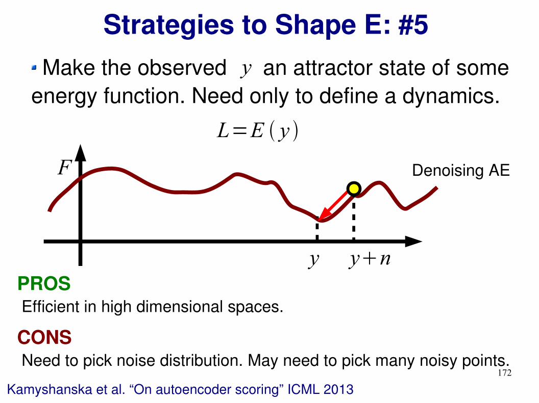
Make the observed an attractor state of some energy function. Need only to define a dynamics.
Strategies to Shape E: #5
PROS Efficient in high dimensional spaces.
CONS Need to pick noise distribution. May need to pick many noisy points.
Kamyshanska et al. “On autoencoder scoring” ICML 2013
Denoising AEF
y
L=E y
y yn
173
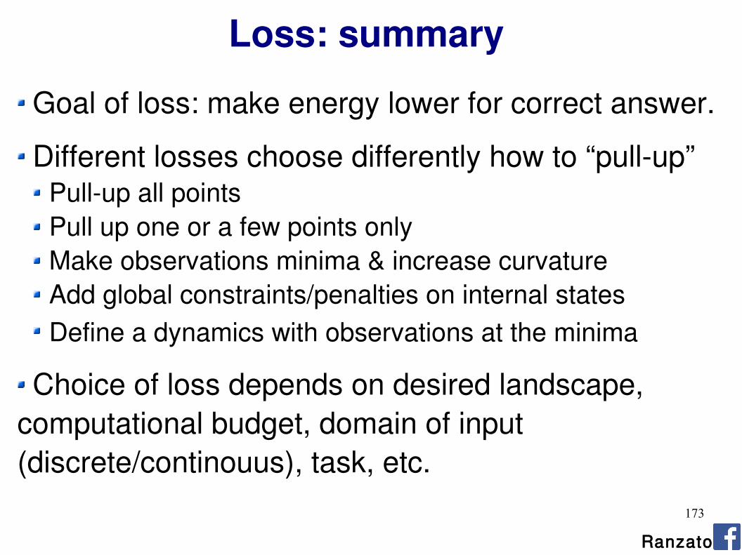
Loss: summary
Goal of loss: make energy lower for correct answer.
Different losses choose differently how to “pull-up”Pull-up all pointsPull up one or a few points onlyMake observations minima & increase curvatureAdd global constraints/penalties on internal statesDefine a dynamics with observations at the minima
Choice of loss depends on desired landscape, computational budget, domain of input (discrete/continouus), task, etc.
Ranzato

174
Final Notes on EBMs
EBMs apply to any predictor (shallow & deep).
EBMs subsume graphical models (e.g., use strategy #1 or #2 to “pull-up”).
EBM is general framework to design good loss functions.
Ranzato

175
Outline
Ranzato
Theory: Energy-Based ModelsEnergy functionLoss function
Examples:Supervised learning: neural netsUnsupervised learning: sparse codingUnsupervised learning: gated MRF
Conclusions
176
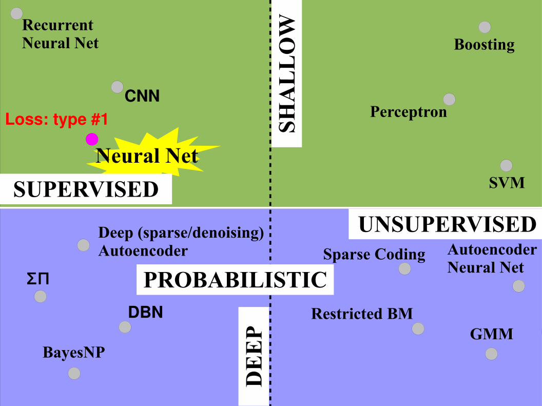
Perceptron
Neural Net
Boosting
SVM
GMM
ΣΠ
BayesNP
CNN
Recurrent Neural Net
AutoencoderNeural Net
Sparse Coding
Restricted BMDBN
Deep (sparse/denoising) Autoencoder
UNSUPERVISED
SUPERVISED
DE
EP
SHA
LL
OW
PROBABILISTIC
Loss: type #1
177
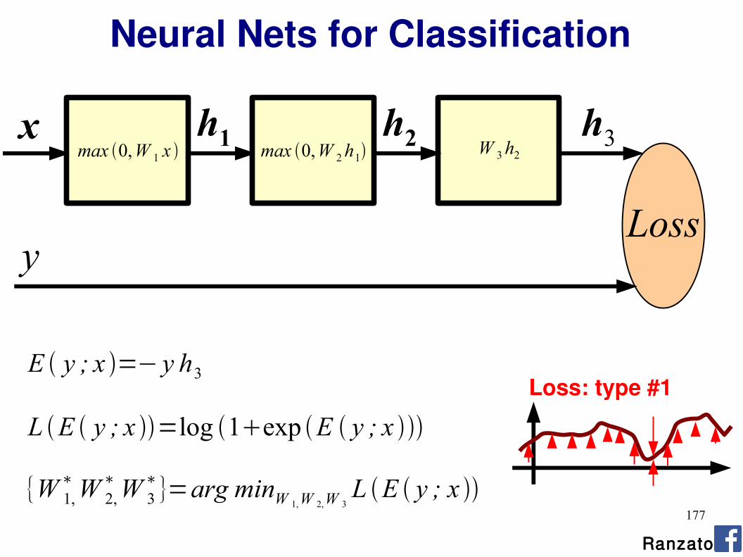
Neural Nets for Classification
h2h1x h3
Lossy
max 0,W 1 x max 0,W 2h1 W 3h2
L E y ; x =log 1exp E y ; x
E y ; x =− y h3
{W 1,∗W 2,
∗W 3∗}=arg minW 1,W 2,W 3
L E y ; x
Loss: type #1
Ranzato

178
Perceptron
Neural Net
Boosting
SVM
GMM
ΣΠ
BayesNP
CNN
Recurrent Neural Net
AutoencoderNeural Net
Sparse Coding
Restricted BMDBN
Deep (sparse/denoising) Autoencoder
UNSUPERVISED
SUPERVISED
DE
EP
SHA
LL
OW
PROBABILISTIC Loss: type #4
179
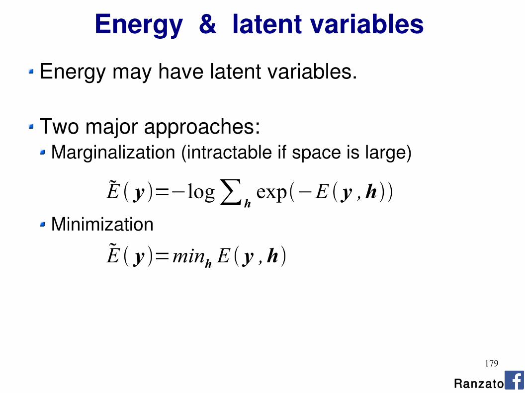
Energy & latent variables
Energy may have latent variables.
Two major approaches:Marginalization (intractable if space is large)
Minimization
E y =minh E y ,h
E y =−log∑hexp−E y ,h
Ranzato

180
Sparse Coding
L= E x ;W
E x ,h ;W =12∥x−W h∥2
2∥h∥1
E x ;W =minhE x ,h ;W Loss type #4: energy loss with (sparsity) constraints.
Ranzato et al. NIPS 2006Olshausen & Field, Nature 1996

181
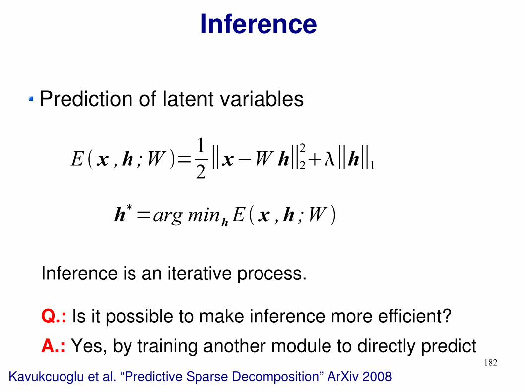
Inference
Prediction of latent variables
h∗=arg minhE x ,h ;W
Inference is an iterative process.
E x ,h ;W =12∥x−W h∥2
2∥h∥1
Ranzato
182
Inference
Prediction of latent variables
h∗=arg minhE x ,h ;W
Inference is an iterative process.
E x ,h ;W =12∥x−W h∥2
2∥h∥1
Q.: Is it possible to make inference more efficient?A.: Yes, by training another module to directly predict
Kavukcuoglu et al. “Predictive Sparse Decomposition” ArXiv 2008

183
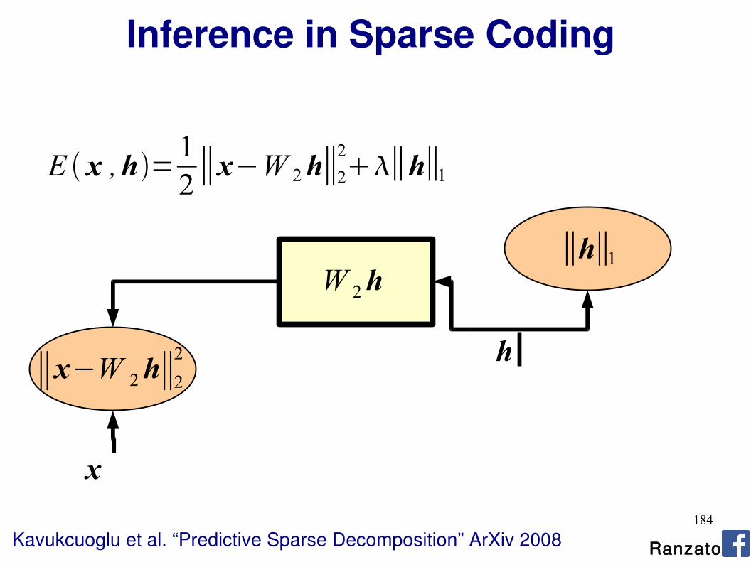
Inference in Sparse Coding
E x ,h=12∥x−W 2h∥2
2∥h∥1
Kavukcuoglu et al. “Predictive Sparse Decomposition” ArXiv 2008
x
h
x
h
Warg minhE
Ranzato
184
E x ,h=12∥x−W 2h∥2
2∥h∥1
Kavukcuoglu et al. “Predictive Sparse Decomposition” ArXiv 2008
W 2h
∥x−W 2h∥22
∥h∥1
h
x
Inference in Sparse Coding
Ranzato

185
Learning To Perform Fast Inference
E x ,h=12∥x−W 2h∥2
2∥h∥1
12∥h−g x ;W 1∥2
2
Kavukcuoglu et al. “Predictive Sparse Decomposition” ArXiv 2008
g x ;W 1
∥h−g x ;W 1∥22
h
x
Ranzato

186
Predictive Sparse Decomposition
E x ,h=12∥x−W 2h∥2
2∥h∥1
12∥h−g x ;W 1∥2
2
Kavukcuoglu et al. “Predictive Sparse Decomposition” ArXiv 2008
g x ;W 1
W 2h
∥x−W 2h∥22
∥h−g x ;W 1∥22
∥h∥1
h
x
Ranzato
187
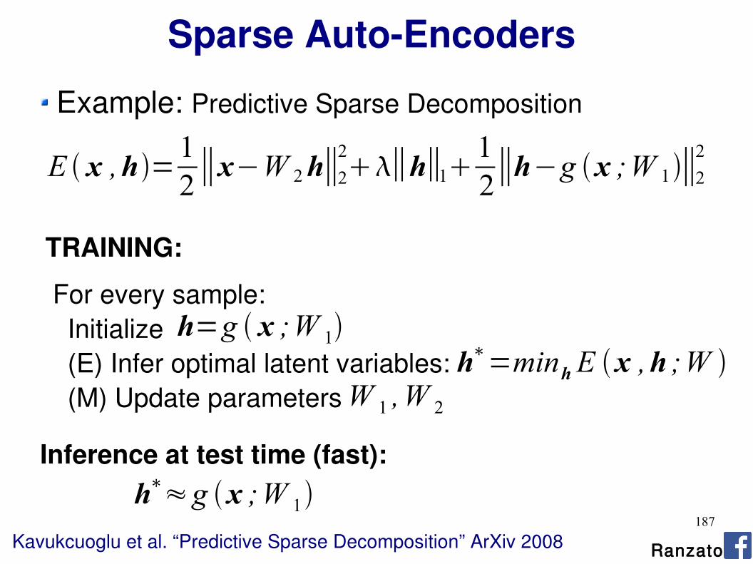
Sparse Auto-Encoders
Example: Predictive Sparse Decomposition
E x ,h=12∥x−W 2h∥2
2∥h∥1
12∥h−g x ;W 1∥2
2
Kavukcuoglu et al. “Predictive Sparse Decomposition” ArXiv 2008
TRAINING:
For every sample: Initialize (E) Infer optimal latent variables: (M) Update parameters
h=g x ;W 1h∗=minhE x ,h ;W
W 1 ,W 2
Inference at test time (fast):h∗≈g x ;W 1
Ranzato

188
E x ,h=12∥x−W 2h∥2
2∥h∥1
12∥h−g x ;W 1∥2
2
Kavukcuoglu et al. “Predictive Sparse Decomposition” ArXiv 2008
x
h
W x h
alternative graphical representations
Predictive Sparse Decomposition
Ranzato
189
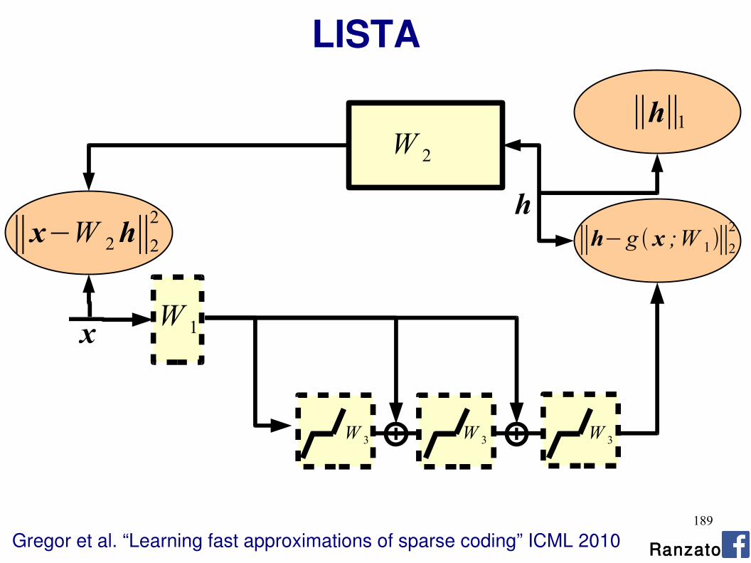
Gregor et al. “Learning fast approximations of sparse coding” ICML 2010
LISTA
W 1
W 2
∥x−W 2h∥22
∥h−g x ;W 1∥22
∥h∥1
h
x
++W 3 W 3 W 3
Ranzato

190
KEY IDEAS
Inference can require expensive optimization
We may approximate exact inference well by using a non-linear function (learn optimal approximation to perform fast inference)
The original model and the fast predictor can be trained jointly
Kavukcuoglu et al. “Predictive Sparse Decomposition” ArXiv 2008
Rolfe et al. “Discriminative Recurrent Sparse Autoencoders” ICLR 2013Szlam et al. “Fast approximations to structured sparse coding...” ECCV 2012Gregor et al. “Structured sparse coding via lateral inhibition” NIPS 2011Kavukcuoglu et al. “Learning convolutonal feature hierarchies..” NIPS 2010
Ranzato
191
Outline
Theory: Energy-Based ModelsEnergy functionLoss function
Examples:Supervised learning: neural netsSupervised learning: convnetsUnsupervised learning: sparse codingUnsupervised learning: gated MRF
Other examples Practical tricks
Ranzato
192
Perceptron
Neural Net
Boosting
SVM
GMM
ΣΠ
BayesNP
CNN
Recurrent Neural Net
AutoencoderNeural Net
Sparse Coding
Restricted BMDBN
Deep (sparse/denoising) Autoencoder
UNSUPERVISED
SUPERVISED
DE
EP
SHA
LL
OW
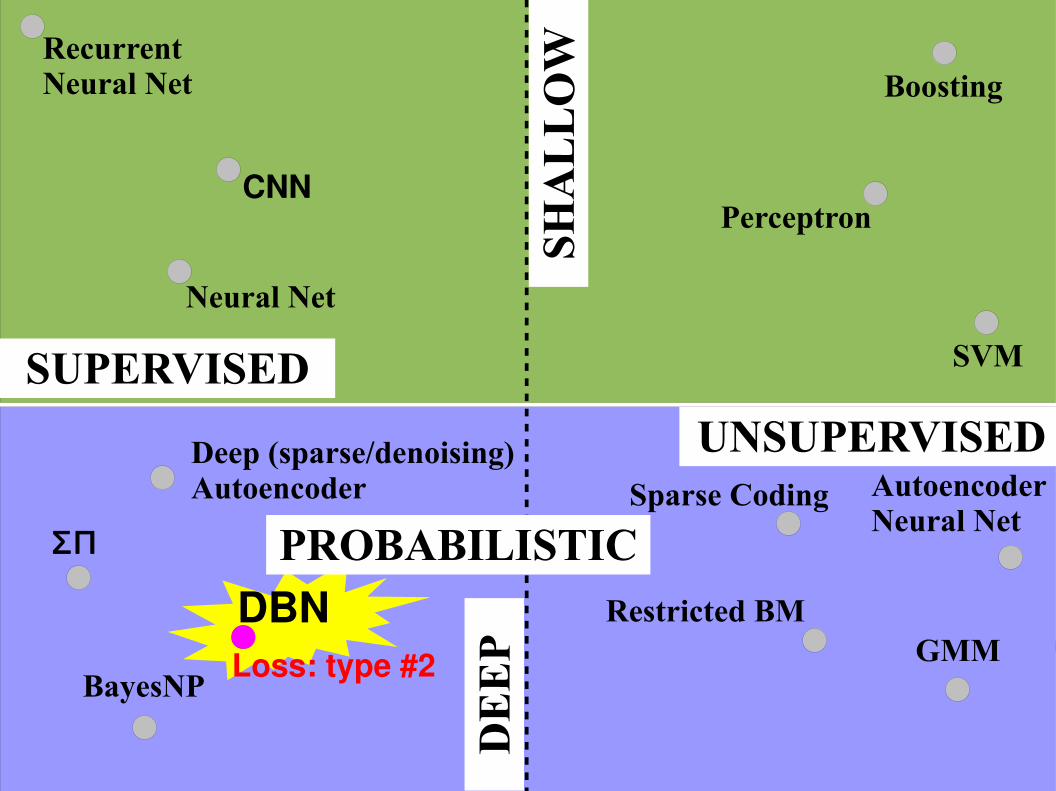
PROBABILISTIC
Loss: type #2
193
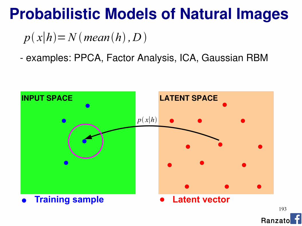
Probabilistic Models of Natural Images
INPUT SPACE LATENT SPACE
Training sample Latent vector
p x∣h=N meanh ,D
- examples: PPCA, Factor Analysis, ICA, Gaussian RBM
p x∣h
Ranzato
194
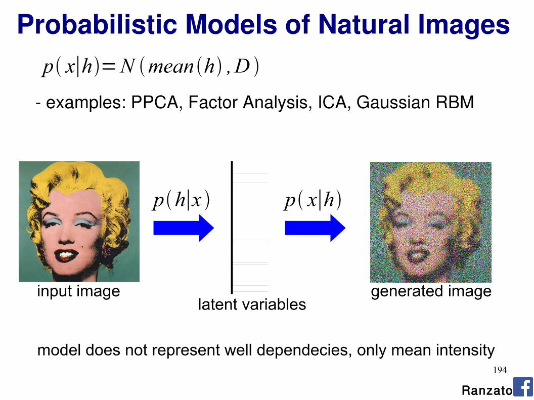
Probabilistic Models of Natural Images
input image
model does not represent well dependecies, only mean intensity
ph∣x p x∣h
generated imagelatent variables
p x∣h=N meanh ,D
- examples: PPCA, Factor Analysis, ICA, Gaussian RBM
Ranzato
195
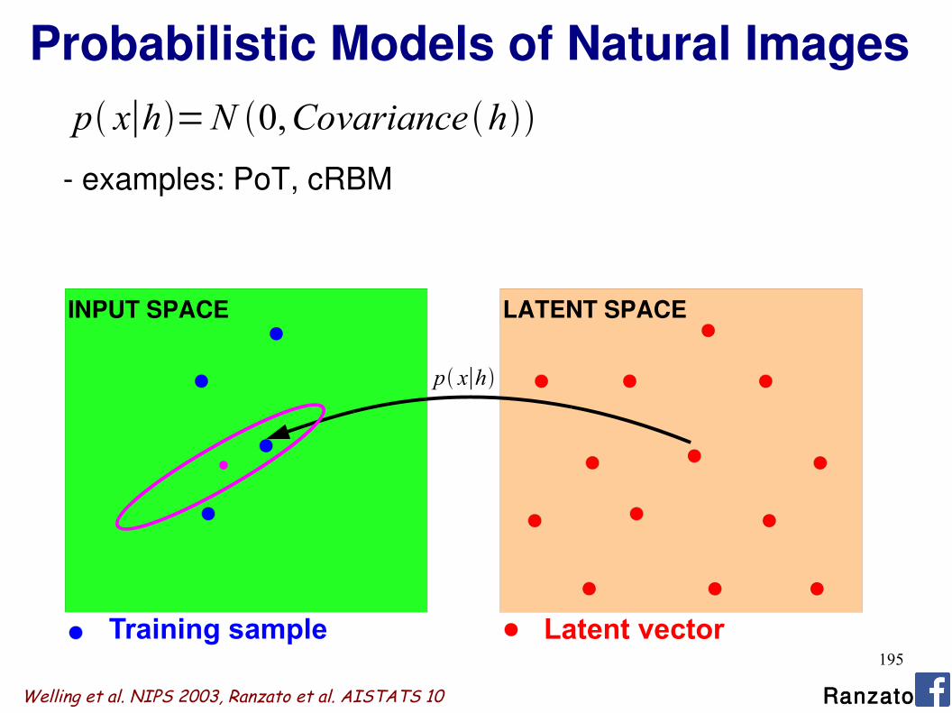
Probabilistic Models of Natural Images
Training sample Latent vector
p x∣h=N 0,Covariance h
- examples: PoT, cRBM
p x∣h
Welling et al. NIPS 2003, Ranzato et al. AISTATS 10
INPUT SPACE LATENT SPACE
Ranzato
196
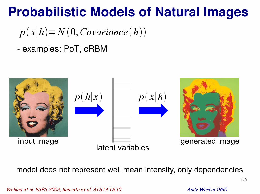
Probabilistic Models of Natural Images
Welling et al. NIPS 2003, Ranzato et al. AISTATS 10
model does not represent well mean intensity, only dependencies
Andy Warhol 1960
input image
ph∣x p x∣h
generated imagelatent variables
p x∣h=N 0,Covariance h
- examples: PoT, cRBM

197
Probabilistic Models of Natural Images
Training sample Latent vector
p x∣h=N mean h ,Covariance h
- this is what we propose: mcRBM, mPoT
Ranzato et al. CVPR 10, Ranzato et al. NIPS 2010, Ranzato et al. CVPR 11
p x∣h
INPUT SPACE LATENT SPACE
Ranzato

198
Probabilistic Models of Natural Images
Training sample Latent vector
Ranzato et al. CVPR 10, Ranzato et al. NIPS 2010, Ranzato et al. CVPR 11
p x∣h
p x∣h=N mean h ,Covariance h
- this is what we propose: mcRBM, mPoT
INPUT SPACE LATENT SPACE
Ranzato
199
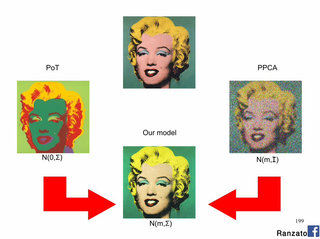
PoT PPCA
Our model
N(0,Σ) N(m,I)
N(m,Σ)Ranzato

200
Deep Gated MRFLayer 1:
E x ,hc, h
m=12x '
−1x
pair-wise MRFx p xq
Ranzato et al. “Modeling natural images with gated MRFs” PAMI 2013
p x ,hc , hm e−E x , hc ,hm
Ranzato
201
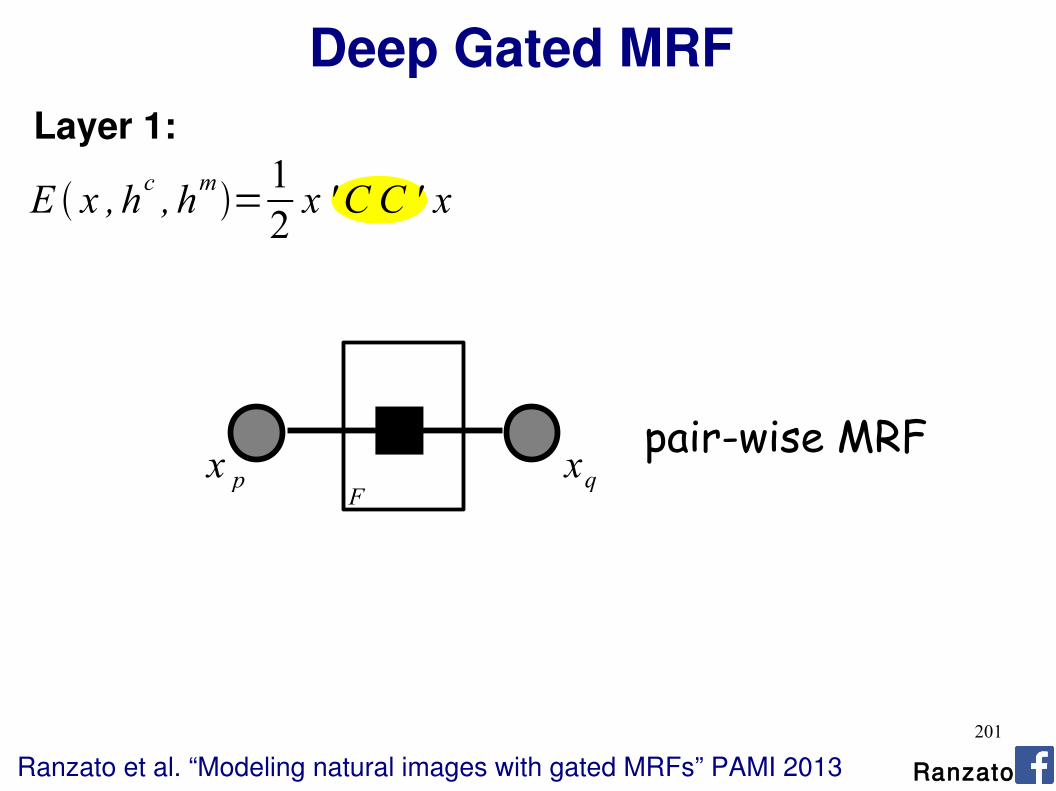
Deep Gated MRFLayer 1:
E x ,hc, h
m=12x ' C C ' x
pair-wise MRFx p xq
F
Ranzato et al. “Modeling natural images with gated MRFs” PAMI 2013 Ranzato
202
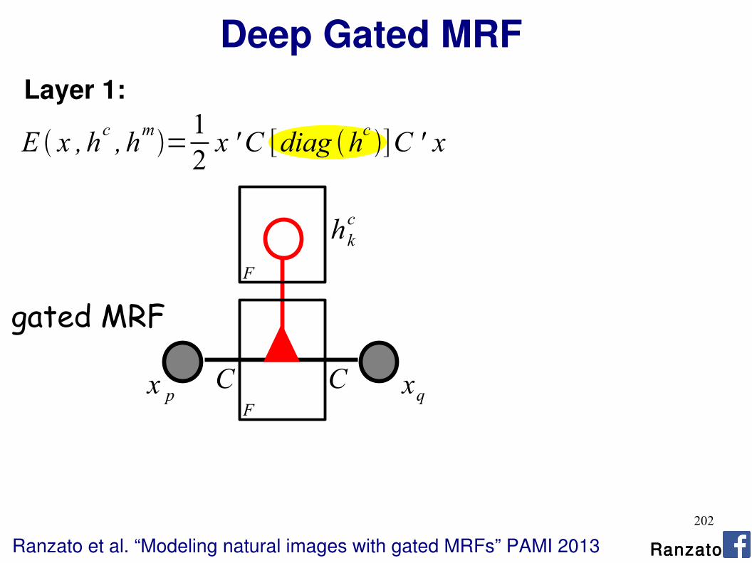
Deep Gated MRFLayer 1:
E x ,hc, h
m=12x ' C [diag h
c]C ' x
gated MRF
x p xq
hkc
CCF
F
Ranzato et al. “Modeling natural images with gated MRFs” PAMI 2013 Ranzato

203
Deep Gated MRF
Ranzato et al. “Modeling natural images with gated MRFs” PAMI 2013
Layer 1:
E x ,hc, h
m=12x ' C [diag h
c]C ' x
12x ' x− x ' W h
m
x p xq
h jm
W
CCF
M
hkc
N
gated MRF
p x ∫hc∫hme−E x ,h
c , hm

204
Deep Gated MRF
Ranzato et al. “Modeling natural images with gated MRFs” PAMI 2013
Layer 1:
E x ,hc, h
m=12x ' C [diag h
c]C ' x
12x ' x− x ' W h
m
Inference of latent variables: just a forward pass
Generation: sampling from multi-variate Gaussian
p x∣hc , hm=N Whm ,
−1=C diag [hc ]C ' I
phkc=1∣x=−
12Pk C ' x
2bk
ph jm=1∣x = W j ' xb j

205
Deep Gated MRF: Training
Ranzato et al. “Modeling natural images with gated MRFs” PAMI 2013
Layer 1:
E x ,hc, h
m=12x ' C [diag h
c]C ' x
12x ' x− x ' W h
m
Training by maximum likelihood (PCD):
p x =∫hm , hc
e−E x , hm , hc
∫x ,hm , hce−E x ,hm ,hc
Loss type #2
Since integrating over the input space is intractable we use:

206
∂ F∂ w
training sample
F= - log(p(x)) + K
p x =e−F x
∫xe−F x
F x =−log∫hm , hce−E x , h
m , hc
free energy

207
HMC dynamics∂ F∂ w
training sample
F= - log(p(x)) + K
p x =e−F x
∫xe−F x
F x =−log∫hm , hce−E x , h
m , hc
free energy

208
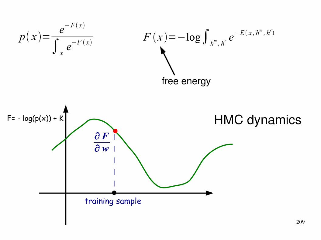
∂ F∂ w
training sample
F= - log(p(x)) + K HMC dynamics
p x =e−F x
∫xe−F x
F x =−log∫hm , hce−E x , h
m , hc
free energy
209
∂ F∂ w
training sample
F= - log(p(x)) + K HMC dynamics
p x =e−F x
∫xe−F x
F x =−log∫hm , hce−E x , h
m , hc
free energy

210
∂ F∂ w
training sample
F= - log(p(x)) + K HMC dynamics
p x =e−F x
∫xe−F x
F x =−log∫hm , hce−E x , h
m , hc
free energy

211
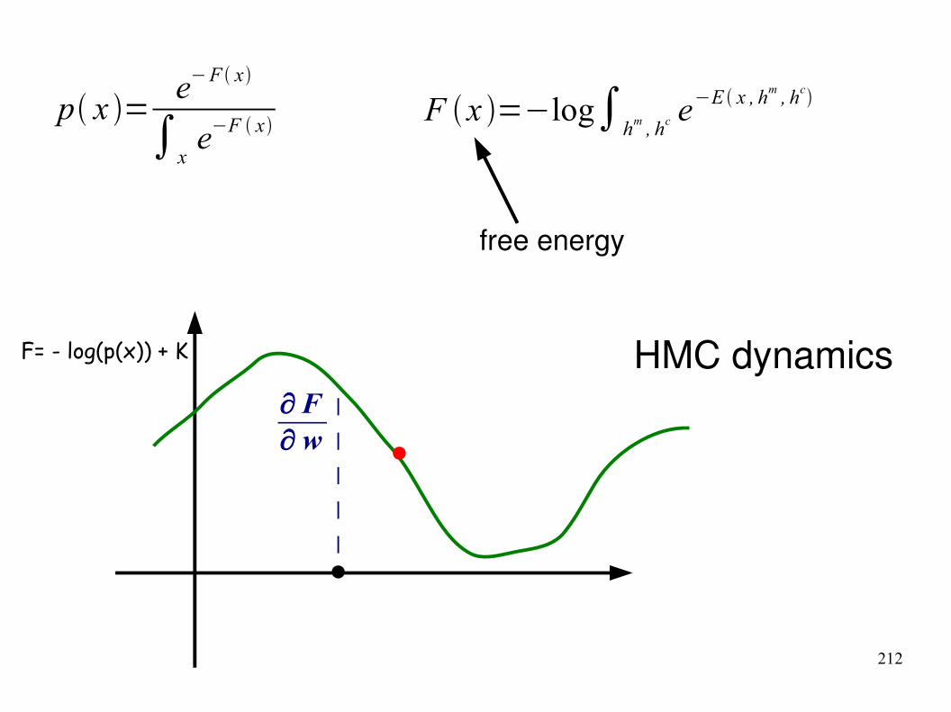
∂ F∂ w
training sample
F= - log(p(x)) + K HMC dynamics
p x =e−F x
∫xe−F x
F x =−log∫hm , hce−E x , h
m , hc
free energy
212
∂ F∂ w
F= - log(p(x)) + K HMC dynamics
p x =e−F x
∫xe−F x
F x =−log∫hm , hce−E x , h
m , hc
free energy

213
∂ F∂ w
weight update∂ F∂ w
sample datapoint
ww− − ∂ F∂ w
∣sample∂ F∂ w
∣data
F= - log(p(x)) + K
p x =e−F x
∫xe−F x
F x =−log∫hm , hce−E x , h
m , hc
free energy

214
∂ F∂ w
∂ F∂ w
sample datapoint
ww− − ∂ F∂ w
∣sample∂ F∂ w
∣data
F= - log(p(x)) + K weight update
p x =e−F x
∫xe−F x
F x =−log∫hm , hce−E x , h
m , hc
free energy
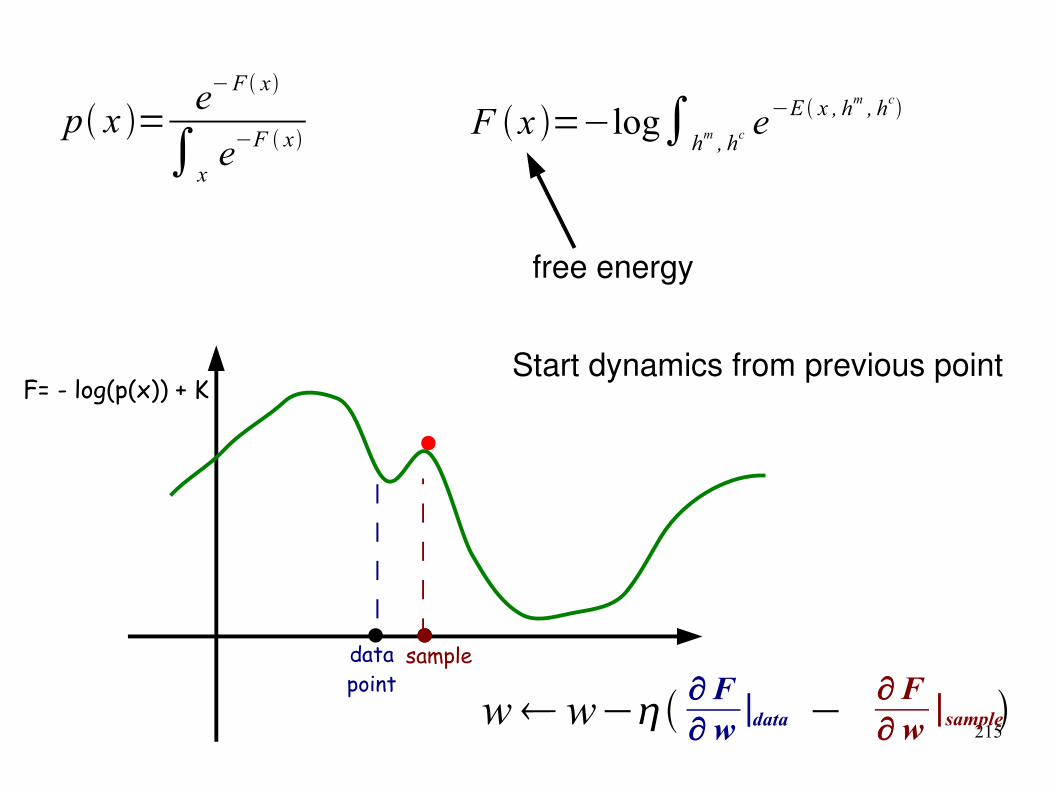
215ww− −
∂ F∂ w
∣sample∂ F∂ w
∣data
Start dynamics from previous point
datapoint
sample
F= - log(p(x)) + K
p x =e−F x
∫xe−F x
F x =−log∫hm , hce−E x , h
m , hc
free energy
216
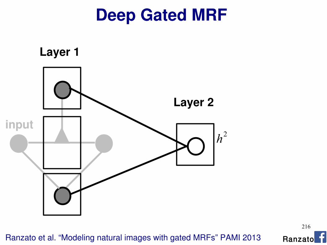
Deep Gated MRF
Ranzato et al. “Modeling natural images with gated MRFs” PAMI 2013
Layer 1
Layer 2
inputh2
Ranzato

217
Deep Gated MRF
Ranzato et al. “Modeling natural images with gated MRFs” PAMI 2013
Layer 1
h2
Layer 2
inputh3
Layer 3
Ranzato

218
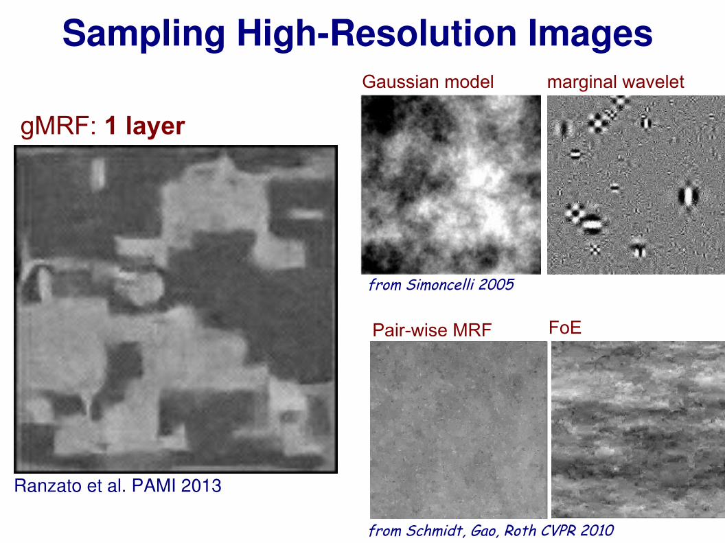
Gaussian model marginal wavelet
from Simoncelli 2005
Pair-wise MRF FoE
from Schmidt, Gao, Roth CVPR 2010
Sampling High-Resolution Images

219
Gaussian model marginal wavelet
from Simoncelli 2005
Pair-wise MRF FoE
from Schmidt, Gao, Roth CVPR 2010
Sampling High-Resolution Images
gMRF: 1 layer
Ranzato et al. PAMI 2013
220
Gaussian model marginal wavelet
from Simoncelli 2005
Pair-wise MRF FoE
from Schmidt, Gao, Roth CVPR 2010
Sampling High-Resolution Images
Ranzato et al. PAMI 2013
gMRF: 1 layer

221
Gaussian model marginal wavelet
from Simoncelli 2005
Pair-wise MRF FoE
from Schmidt, Gao, Roth CVPR 2010
Sampling High-Resolution Images
Ranzato et al. PAMI 2013
gMRF: 1 layer

222
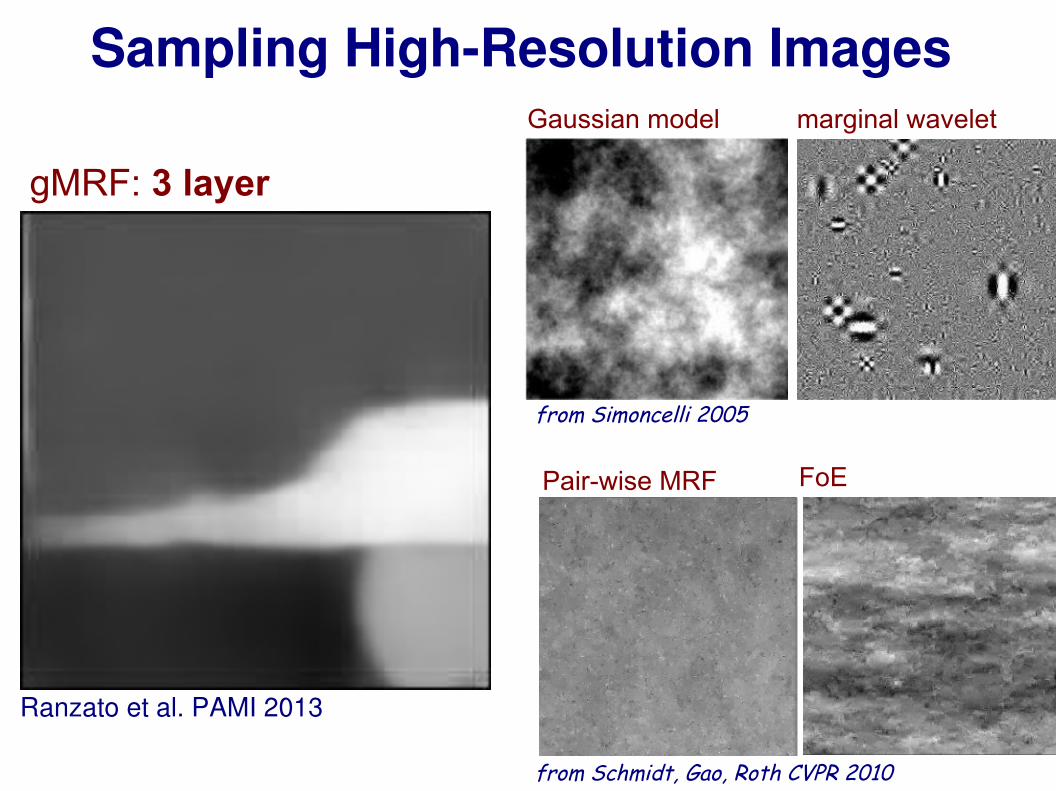
Gaussian model marginal wavelet
from Simoncelli 2005
Pair-wise MRF FoE
from Schmidt, Gao, Roth CVPR 2010
Sampling High-Resolution Images
Ranzato et al. PAMI 2013
gMRF: 3 layer
223
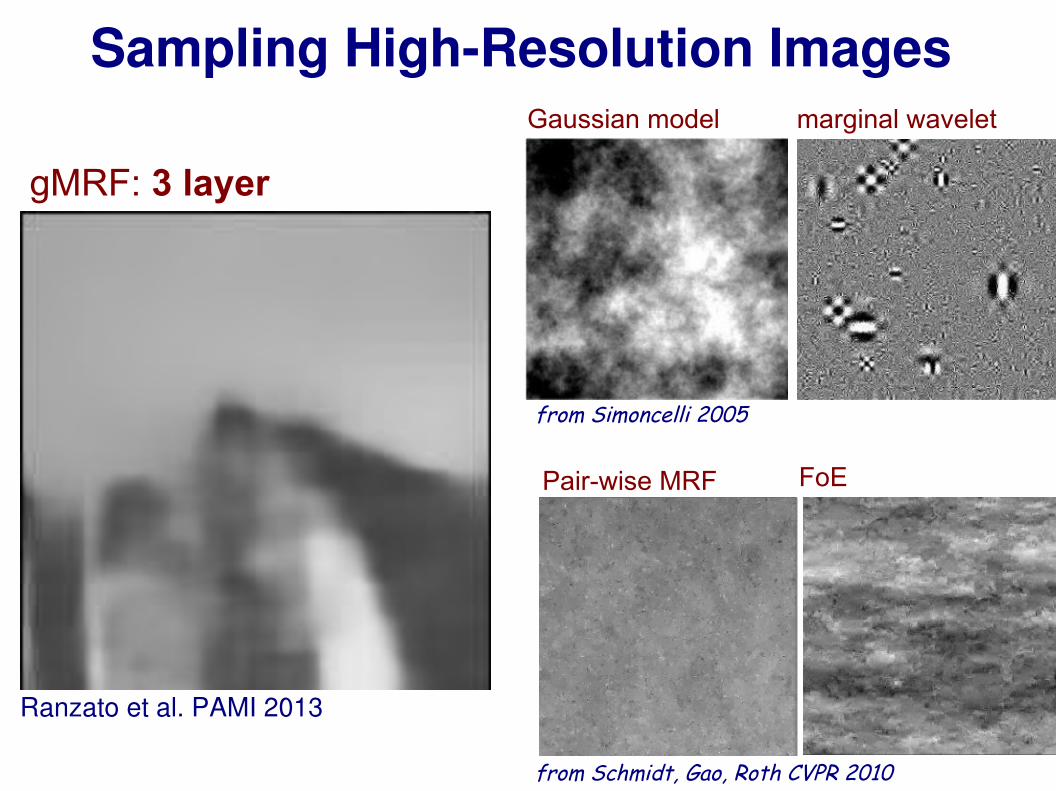
Gaussian model marginal wavelet
from Simoncelli 2005
Pair-wise MRF FoE
from Schmidt, Gao, Roth CVPR 2010
Sampling High-Resolution Images
Ranzato et al. PAMI 2013
gMRF: 3 layer
224
Gaussian model marginal wavelet
from Simoncelli 2005
Pair-wise MRF FoE
from Schmidt, Gao, Roth CVPR 2010
Sampling High-Resolution Images
Ranzato et al. PAMI 2013
gMRF: 3 layer

225
Gaussian model marginal wavelet
from Simoncelli 2005
Pair-wise MRF FoE
from Schmidt, Gao, Roth CVPR 2010
Sampling High-Resolution Images
Ranzato et al. PAMI 2013
gMRF: 3 layer

226
Sampling After Training on Face Images
Original Input 1st layer 2nd layer 3rd layer 4th layer 10 times
unconstrained samples
conditional (on the left part of the face) samples
Ranzato et al. PAMI 2013 Ranzato
227
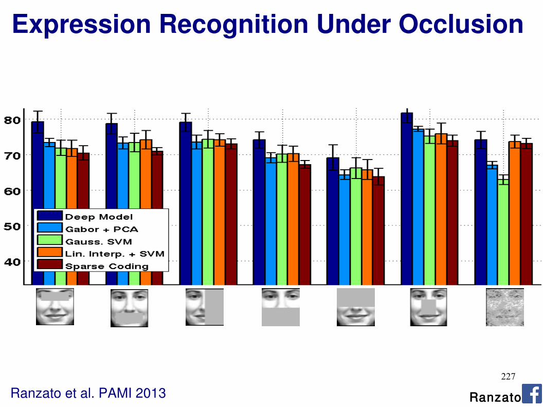
Expression Recognition Under Occlusion
Ranzato et al. PAMI 2013 Ranzato

228
Tang et al. Robust BM for decognition and denoising CVPR 2012 Ranzato

229
Pros Cons Feature extraction is fast Unprecedented generation
quality Advances models of natural
images Trains without labeled data
Training is inefficientSlowTricky
Sampling scales badly with dimensionality What's the use case of
generative models?
Conclusion If generation is not required, other feature learning methods are
more efficient (e.g., sparse auto-encoders). What's the use case of generative models? Given enough labeled data, unsup. learning methods have not produced more useful features.
230
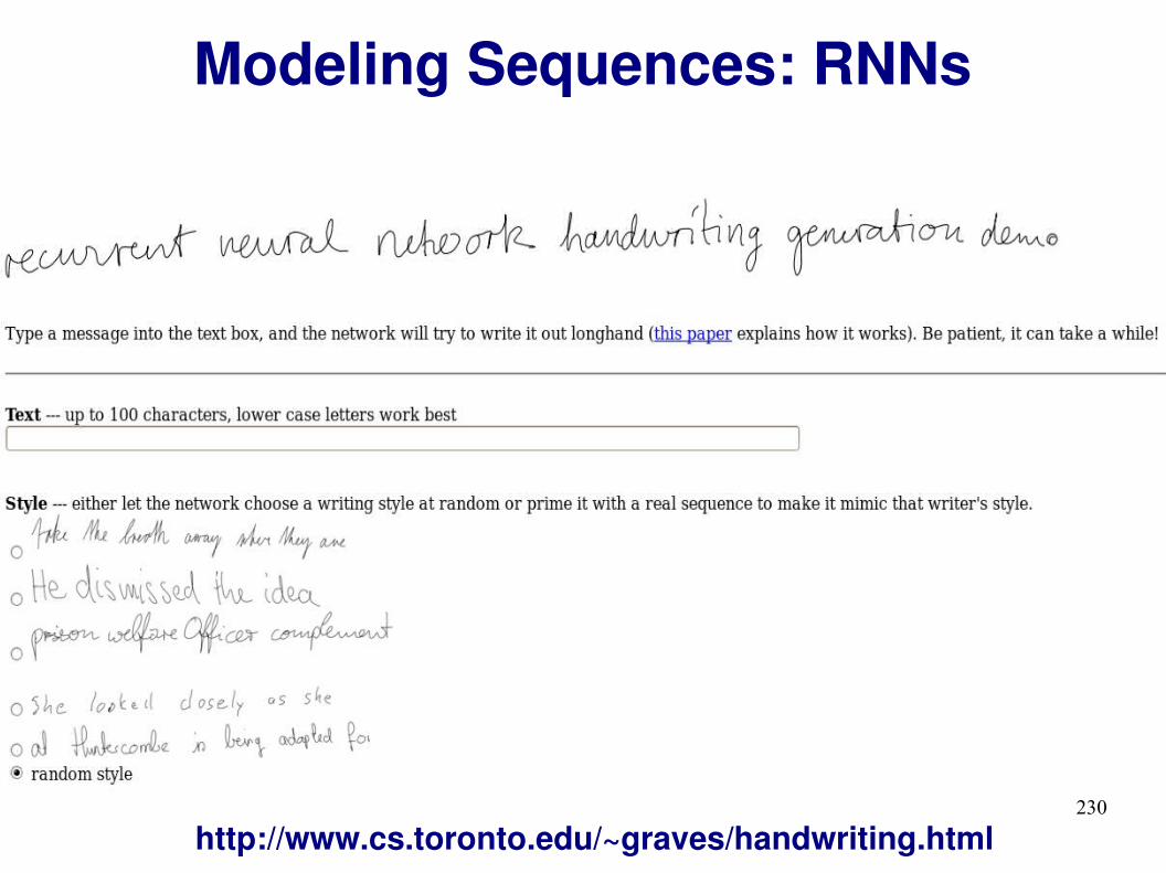
Modeling Sequences: RNNs
http://www.cs.toronto.edu/~graves/handwriting.html

231
Structured Prediction: GTN
LeCun et al. “Gradient-based learning applied to document recognition” IEEE 1998
232
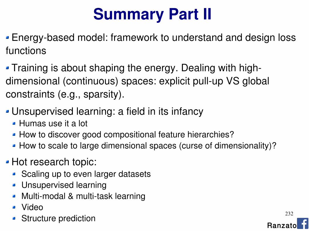
Summary Part II Energy-based model: framework to understand and design loss
functions
Training is about shaping the energy. Dealing with high-dimensional (continuous) spaces: explicit pull-up VS global constraints (e.g., sparsity).
Unsupervised learning: a field in its infancyHumas use it a lotHow to discover good compositional feature hierarchies?How to scale to large dimensional spaces (curse of dimensionality)?
Hot research topic: Scaling up to even larger datasets Unsupervised learning Multi-modal & multi-task learning Video Structure prediction
Ranzato

233
Questions A ReLU layer computes: h = max(0, W x + b), where x is a D dimensional vector, h
and b are N dimensional vectors and W is a matrix of size NxD. If dL/dh is the derivative of the loss w.r.t. h, then backpropagation computes (in matlab notation):
a) the derivatives dL/dx = W' (dL/dh .* 1(h)), where 1(h) = 1 if h>0 o/w it is 0 b) the derivatives dL/dW = (dL/dh .* 1(h)) x' and dL/db = dL/dh .* 1(h)c) both the derivatives in a) and b)
Ranzato
A convolutional network:a) is well defined only when layers are everywhere differentiableb) requires unsupervised learning even if the labeled dataset is very largec) has usually many convolution/pooling/normalization layers followed by fully connected layers
Sparse coding:a) aims at extracting sparse features that are good at reconstructing the input and it does not need labels for training; the dimensionality of the feature vector is usually higher than the input. b) requires to have lots of images with their corresponding labelsc) can be interpreted as a graphical model, and inference of the latent variables (sparse codes) is done by marginalization.

234
THANK YOU
Ranzato