lecture 1: course logistics, introduction, bias-variance
TRANSCRIPT

Lecture 1: Course logistics, introduction,bias-variance tradeoff
STATS 202: Data Mining and Analysis
Linh [email protected]
Department of StatisticsStanford University
June 21, 2021
STATS 202: Data Mining and Analysis L. Tran 1/51

Course Information
I Class website: stats-202.github.io
I Videos: Zoom lectures will be recorded/uploaded to Canvas.
I Textbook: An Introduction to Statistical Learning
I Supplemental Textbook: The Elements of StatisticalLearning
I Email policy: Please use Piazza for most questions.Homeworks and Exams should be submitted via Gradescope.
I Office hours: Please refer to this Google calendar.
STATS 202: Data Mining and Analysis L. Tran 2/51

Syllabus
I Topics: Intro to statistical learning and methods for analyzinglarge amounts of data
I Prereqs: STATS 60, MATH 51, CS 105
I Grades: 3 components
I 4 homework assignments (50pts each)
I Due by 3:59pm PDT of due date
I Accepted up to 2-days late w/ 20% penalty (2 free late days)
I Take home midterm on Wednesday, July 21 (100pts)
I Final project (200pts)
I Submissions due on Monday, August 23, 2021
I Write-up due on Friday, August 27, 2021
STATS 202: Data Mining and Analysis L. Tran 3/51

Class material
STATS 202: Data Mining and Analysis L. Tran 4/51
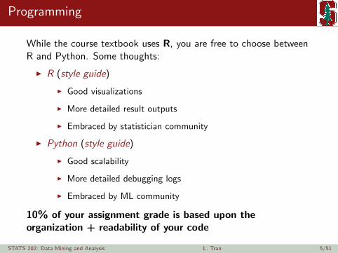
Programming
While the course textbook uses R, you are free to choose betweenR and Python. Some thoughts:
I R (style guide)
I Good visualizations
I More detailed result outputs
I Embraced by statistician community
I Python (style guide)
I Good scalability
I More detailed debugging logs
I Embraced by ML community
10% of your assignment grade is based upon theorganization + readability of your code
STATS 202: Data Mining and Analysis L. Tran 5/51

Motivation
Companies are paying lots of money for statistical models.
I Netflix
I Heritage Provider Network
I Department of Homeland Security
I Zillow
I Etc...
STATS 202: Data Mining and Analysis L. Tran 6/51

Netflix
Popularized prediction challenges by organizing an open, blindcontest to improve its recommendation system.
I Prize: $1 million
I Features: User ratings (1 to 5 stars) on previously watchedfilms
I Outcome: User ratings (1 to 5 stars) for unwatched films
STATS 202: Data Mining and Analysis L. Tran 7/51

Heritage Provider Network
Ran for two years, with six milestone prizes during that span.
I Prize: $3 million ($500K)
I Features: Anonymized patient data over a 48 month period
I Outcome: How many days a patient will spend in a hospitalin the next year
STATS 202: Data Mining and Analysis L. Tran 8/51
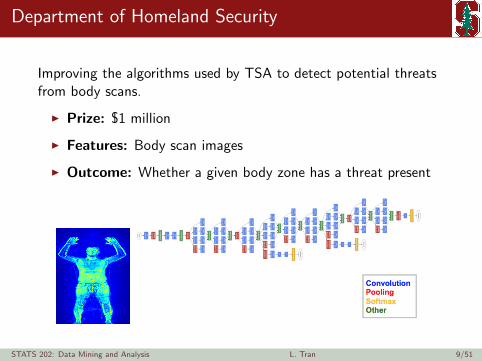
Department of Homeland Security
Improving the algorithms used by TSA to detect potential threatsfrom body scans.
I Prize: $1 million
I Features: Body scan images
I Outcome: Whether a given body zone has a threat present
STATS 202: Data Mining and Analysis L. Tran 9/51
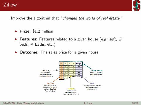
Zillow
Improve the algorithm that “changed the world of real estate.”
I Prize: $1.2 million
I Features: Features related to a given house (e.g. sqft, #beds, # baths, etc.)
I Outcome: The sales price for a given house
STATS 202: Data Mining and Analysis L. Tran 10/51
Empirical vs true distributions
Common scenario: I have a data set. What do I do?Common approaches:
I Fit a linear model and look at p-values
I Fit a non-parametric model and get predictions
I Calculate summary statistics and form a story around theanswers
STATS 202: Data Mining and Analysis L. Tran 11/51

Empirical vs true distributions
Common scenario: I have a data set. What do I do?Common approaches:
I Fit a linear model and look at p-values
I Fit a non-parametric model and get predictions
I Calculate summary statistics and form a story around theanswers
Can result in significantly different answers!
STATS 202: Data Mining and Analysis L. Tran 12/51

Empirical vs true distributions
Ideally, we want Ψ(P0).
STATS 202: Data Mining and Analysis L. Tran 13/51
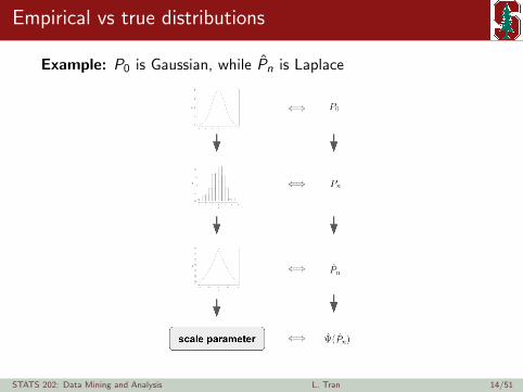
Empirical vs true distributions
Example: P0 is Gaussian, while Pn is Laplace
STATS 202: Data Mining and Analysis L. Tran 14/51
Applied example
The financial crisis of 2007-2008.I Let O = (X1,X2, ...,Xp,Y ) be our data
I e.g. X’s are measures of financial & real estate market. Y isCDO value.
I Generally want to estimate E0[Y |X1,X2, ...,Xp]
I Two big issues:
1. Pn wasn’t representative of P0
2. Most statistical models assume Oiiid∼ P0
Result: Ψ(P0) was no where close to Ψ(Pn)
STATS 202: Data Mining and Analysis L. Tran 15/51

Supervised vs unsupervised learning
Supervised: We have a clearly defined outcome of interest.
I Pro: More clearly defined
I Con: May take more resources to gather
Unsupervised: We don’t have a clearly defined outcome ofinterest.
I Pro: Typically readily available
I Con: May be a more abstract problem
STATS 202: Data Mining and Analysis L. Tran 16/51

Unsupervised learning
Typically start with a data matrix, e.g.
*n.b. The data may also be unstructured (e.g. text, pixels,etc).
STATS 202: Data Mining and Analysis L. Tran 17/51
Unsupervised learning
Two primary categories:
1. Quantitative:
I Numerical
I Ordinal
2. Qualitative:
I Categorical
I Free form
STATS 202: Data Mining and Analysis L. Tran 18/51

Unsupervised learning
Goal: Learn the overall structure of our data. e.g.
I Clustering: learn meaningful groupings of the data
I e.g. k-means, Expectation Maximization, etc.
I Correlation: learn meaningful relationships between variablesor units
I e.g. concordance, Pearson’s, etc.
I Dimension reduction: learn compression of data fordownstream tasks
I e.g. PCA, LDA, auto-encoding, etc.
We learn these using our data.
STATS 202: Data Mining and Analysis L. Tran 19/51
Supervised learning
Typically start with a data matrix with an outcome, e.g.
Outcome can be quantitative or qualitative.
STATS 202: Data Mining and Analysis L. Tran 20/51

Supervised learning
Goal: We learn a mapping from input variables to outputvariables.
I If quantitative, then we refer to this as Regression
I e.g. E0[Y |X1,X2, ...,Xp]
I If qualitative, then we refer to this as Classification
I e.g. P0[Y = y |X1,X2, ...,Xp]
In both cases, we’re interested in learning some function,
f0(X1,X2, ...,Xp) (1)
We estimate f0 using our data.
STATS 202: Data Mining and Analysis L. Tran 21/51
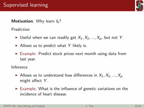
Supervised learning
Motivation: Why learn f0?
Prediction
I Useful when we can readily get X1,X2, ...,Xp, but not Y .
I Allows us to predict what Y likely is.
I Example: Predict stock prices next month using data fromlast year.
Inference
I Allows us to understand how differences in X1,X2, ...,Xp
might affect Y .
I Example: What is the influence of genetic variations on theincidence of heart disease.
STATS 202: Data Mining and Analysis L. Tran 22/51
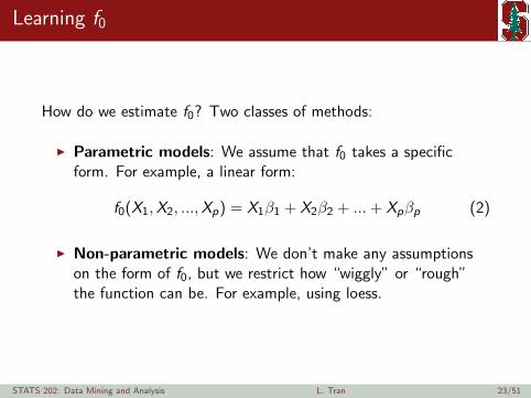
Learning f0
How do we estimate f0? Two classes of methods:
I Parametric models: We assume that f0 takes a specificform. For example, a linear form:
f0(X1,X2, ...,Xp) = X1β1 + X2β2 + ...+ Xpβp (2)
I Non-parametric models: We don’t make any assumptionson the form of f0, but we restrict how “wiggly” or “rough”the function can be. For example, using loess.
STATS 202: Data Mining and Analysis L. Tran 23/51

Parametric vs non-parametric models
Visualization
Non-parametric models tend to be larger than parametric models.
Recall: A statistical model is simply a set of probabilitydistributions that you allow your data to follow.
STATS 202: Data Mining and Analysis L. Tran 24/51
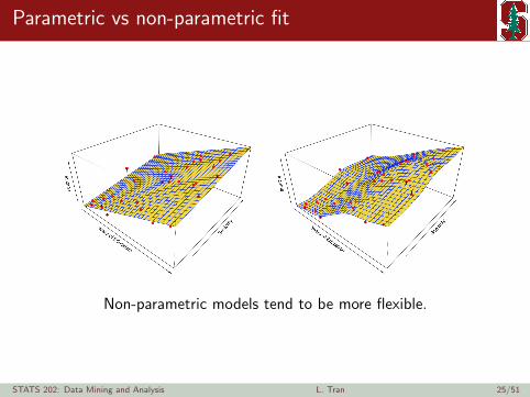
Parametric vs non-parametric fit
Non-parametric models tend to be more flexible.
STATS 202: Data Mining and Analysis L. Tran 25/51

Parametric vs non-parametric models
Question: Why don’t we just always use non-parametric models?
1. Interpretability: parametric models are simpler to interpret
2. Convenience: less computation, more reproducibility, betterbehavior
3. Overfitting: non-parametric models tend to overfit (aka. highvariance)
STATS 202: Data Mining and Analysis L. Tran 26/51

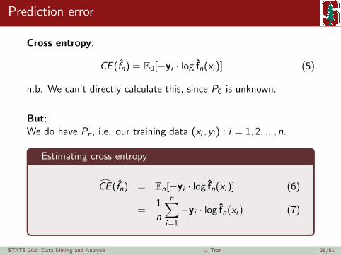
Prediction error
Training data: (xi , yi ) : i = 1, 2, ..., nGoal: Estimate f0 with our data, resulting in fn
Typically: we get fn by minimizing a prediction error
I Assumes (xi , yi )iid∼ P0
Standard prediction error functions:
I Classification: Cross-entropy
CE (fn) = E0[−yi · log fn(xi )] (3)
I Regression: Mean squared error
MSE (fn) = E0[yi − fn(xi )]2 (4)
STATS 202: Data Mining and Analysis L. Tran 27/51

Prediction error
Cross entropy:
CE (fn) = E0[−yi · log fn(xi )] (5)
n.b. We can’t directly calculate this, since P0 is unknown.
But:We do have Pn, i.e. our training data (xi , yi ) : i = 1, 2, ..., n.
Estimating cross entropy
CE (fn) = En[−yi · log fn(xi )] (6)
=1
n
n∑i=1
−yi · log fn(xi ) (7)
STATS 202: Data Mining and Analysis L. Tran 28/51
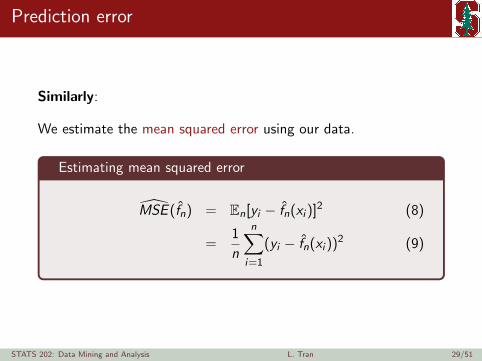
Prediction error
Similarly:
We estimate the mean squared error using our data.
Estimating mean squared error
MSE (fn) = En[yi − fn(xi )]2 (8)
=1
n
n∑i=1
(yi − fn(xi ))2 (9)
STATS 202: Data Mining and Analysis L. Tran 29/51

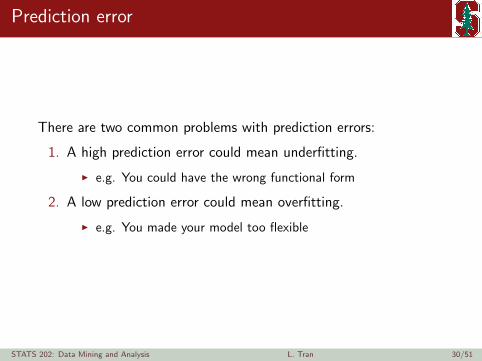
Prediction error
There are two common problems with prediction errors:
1. A high prediction error could mean underfitting.
I e.g. You could have the wrong functional form
2. A low prediction error could mean overfitting.
I e.g. You made your model too flexible
STATS 202: Data Mining and Analysis L. Tran 30/51
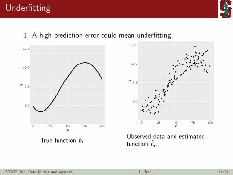
Underfitting
1. A high prediction error could mean underfitting.
5.0
7.5
10.0
12.5
0 25 50 75 100x
y
True function f0.
●
●
●
●
●
●
●
●
●
●
●
●
●
●
●
●
●
●
●
●
●
●
●
●
●
●
●
●
●
●
●
●
●
●
●
●
●
●
●
●
●
●
●
●
●
●
●
●
●
●
●
●
●
●
●
●
●
●
●
●
●
●
●
●
●
●
●
●
●
●
●
●
●
●
●
●
●
●
●
●
●
●
●
●
●
●
●
●
●
●
●
●
●
●●
●
●
●
●
●
5.0
7.5
10.0
12.5
0 25 50 75 100x
y
Observed data and estimatedfunction fn.
STATS 202: Data Mining and Analysis L. Tran 31/51
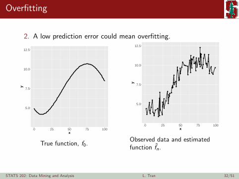
Overfitting
2. A low prediction error could mean overfitting.
5.0
7.5
10.0
12.5
0 25 50 75 100x
y
True function, f0.
●
●
●
●
●
●
●
●
●
●
●
●
●
●
●
●
●
●
●
●
●
●
●
●
●
●
●
●
●
●
●
●
●
●
●
●
●
●
●
●
●
●
●
●
●
●
●
●
●
●
●
●
●
●
●
●
●
●
●
●
●
●
●
●
●
●
●
●
●
●
●
●
●
●
●
●
●
●
●
●
●
●
●
●
●
●
●
●
●
●
●
●
●
●●
●
●
●
●
●
5.0
7.5
10.0
12.5
0 25 50 75 100x
y
Observed data and estimatedfunction fn.
STATS 202: Data Mining and Analysis L. Tran 32/51

Prediction error
How to tell if we’ve under/overfit:
I Evaluate on data not used in training (i.e. from your test set).
Given our test data (xi′, yi
′) : i = 1, 2, ...,m, we can calculate amore accurate prediction error, e.g.:
MSE (fn) = Etestn [yi
′− fn(xi′)]2 (10)
=1
m
m∑i=1
(yi′− fn(xi
′))2 (11)
STATS 202: Data Mining and Analysis L. Tran 33/51
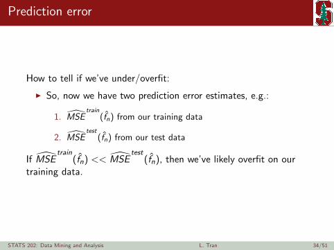
Prediction error
How to tell if we’ve under/overfit:
I So, now we have two prediction error estimates, e.g.:
1. MSEtrain
(fn) from our training data
2. MSEtest
(fn) from our test data
If MSEtrain
(fn) << MSEtest
(fn), then we’ve likely overfit on ourtraining data.
STATS 202: Data Mining and Analysis L. Tran 34/51

How to tell if we’ve under/overfit:
●
●
●
●
●
●
●
●
●
●
●
●
●
●
●
●
●
●
●
●
●
●
●
●●
●
●
●●
●●
●
●
●
●
●
●
●
●●
●
●●●
●
●
●
●
●
●●
●
●
●
●
●
●
●
●
●
●
●
●
●
●●
●●
●
●
●
●
● ●●
●
●●
●
●
●
●
●
●
●
●
●
●●
●
●
●
●
●
●
●
●
●
●
●
5.0
7.5
10.0
12.5
0 25 50 75 100x
y
factor(flexibility)
1
4
4.33
5
7
13
Estimates fn of f0.
●
●
●●
●
●
●
●
●●
●
●
0.5
1.0
1.5
1 2 3 4 5 6 7 8 9 10 11 12 13flexibility
MS
E Data
●
●
Test MSE
Train MSE
MSE for each fn.
STATS 202: Data Mining and Analysis L. Tran 35/51
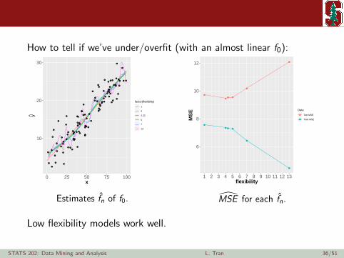
How to tell if we’ve under/overfit (with an almost linear f0):
●
●
●
●
●
●
●
●
●
●
●
●
●
●
●
●
●
●
●
●
●
●
●
●
●
●
●
●●
●●
●
●
●
●
●
●
●
●●
●
●●
●
●
●
●
●
●
●●
●
●
●
●
●
●
●
●
●
●
●
●
●
●●
●●
●
●
●
●
●
●
●
●
●●
●
●
●
●
●
●
●
●
● ●●
●
●
●
●
●
●
●
●
● ●
10
20
30
0 25 50 75 100x
y
factor(flexibility)
1
4
4.33
5
7
13
Estimates fn of f0.
●
●
●●●
●
●
●
●●●
●
6
8
10
12
1 2 3 4 5 6 7 8 9 10 11 12 13flexibility
MS
E Data
●
●
Test MSE
Train MSE
MSE for each fn.
Low flexibility models work well.
STATS 202: Data Mining and Analysis L. Tran 36/51
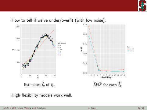
How to tell if we’ve under/overfit (with low noise):
●
●●
●
●●
●
●
●
●
●
●
●●
●
●
●
●
●
●
●
●
● ●
●
●●●●●●
●
●
●
●●
●
●
●●
●
●●●
● ●
●
●●
●●
● ●
●●
● ●●
●
●
●●
●
●●●
●●
●
●●
●
● ●●
●
●●
●●●
●
●
●
●
●
●
●●●
●
●
●
●
●●
●
●
●
●
5.0
7.5
10.0
12.5
0 25 50 75 100x
y
factor(flexibility)
1
4
4.33
5
7
13
Estimates fn of f0.
●●●
●
●
●
●●●
●
●
●
0.00
0.25
0.50
0.75
1.00
1.25
1 2 3 4 5 6 7 8 9 10 11 12 13flexibility
MS
E Data
●
●
Test MSE
Train MSE
MSE for each fn.
High flexibility models work well.
STATS 202: Data Mining and Analysis L. Tran 37/51
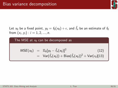
Bias variance decomposition
Let x0 be a fixed point, y0 = f0(x0) + ε, and fn be an estimate of f0from (xi , yi ) : i = 1, 2, ..., n.
The MSE at x0 can be decomposed as
MSE (x0) = E0[y0 − fn(x0)]2 (12)
= Var(fn(x0)) + Bias(fn(x0))2 + Var(ε0)(13)
STATS 202: Data Mining and Analysis L. Tran 38/51
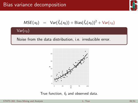
Bias variance decomposition
MSE (x0) = Var(fn(x0)) + Bias(fn(x0))2 + Var(ε0)
Var(ε0)
Noise from the data distribution, i.e. irreducible error.
●
●
●
●
●
●
●
●
●
●
●
●
●
●
●
●
●
●
●
●
●
●
●
●●
●
●
●●
●●
●
●
●
●
●
●
●
●●
●
●●
●
●
●
●
●
●
●●
●
●
●
●
●
●
●●
●
●●
●
●
●●
●●
●
●
●
●
●
●●
●
●●
●
●
●
●
●
●
●
●
●●●
●
●
●
●
●
●
●
●
●
●●
0
10
20
30
40
0 25 50 75 100x
y
True function, f0 and observed data.
STATS 202: Data Mining and Analysis L. Tran 39/51

Bias variance decomposition
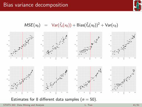
MSE (x0) = Var(fn(x0)) + Bias(fn(x0))2 + Var(ε0)
Var(fn(x0))
The variance of fn(x0) (i.e. the estimate of y).How much the estimate fn at x0 changes with new data.
●●
●
●
●
●
●
●
●
●
●●
●
●
●
●●
●●
●●
●
●
●
●●
●
●
●
●
●
●
●
●
●
●
●
●
●
●
●
●
●
●
●
●
●
●
●
●
0
10
20
30
40
0 25 50 75 100x
y
Observed data and estimate fn.
STATS 202: Data Mining and Analysis L. Tran 40/51
Bias variance decomposition
MSE (x0) = Var(fn(x0)) + Bias(fn(x0))2 + Var(ε0)
●●
●
●
●
●
●
●
●
●
●●
●
●
●
●●
●●
●●
●
●
●
●●
●
●
●
●
●
●
●
●
●
●
●
●
●
●
●
●
●
●
●
●
●
●
●
●
0
10
20
30
40
0 25 50 75 100x
y
●
●
●
●
●
●
●
●
●●
●
●
●
●
●
●
●
●
●
●
●
●●
●
●
●
●
●
●●
●
●
●
●
●
●
●
●
●
●
●
●
●
●●
●
●
●
●
0
10
20
30
40
0 25 50 75 100x
y
●
●●
●
●
●●●●
●
●
●
●
●
●●
●
●
●
●
●
●
●
●
●
●
●
●
●
●
●
●
●
●
●
●
●
●
●
●
●
●
●
●
●●
●
●
●●
0
10
20
30
40
0 25 50 75 100x
y
●
● ●
●
●
●
●
●
●
●
●
●
●
●
●
●
●
●
●
●●
● ●
●
●
●●
●
●
●
●●
●
●
●
●
●
●
●
●●●
●●
●
●
●
●
●
●
0
10
20
30
40
0 25 50 75 100x
y
●
●
●
● ●
●
●
●
●
●
●
●
●
●
●
●
●
●
●
●
●
●
●●
●
●
●
●
●
●
●
●
●
●
●
●
●
●
●
●
●
●
●●
●
●●
●
●
●
0
10
20
30
40
0 25 50 75 100x
y
●
●
●
●
●●
●
●●
●
●
●
●
●
●
●
●●
●
●●
●
●
●
●
●
●
●
●
●
●
●●
●
●
●
●
●
●
●
●
●
●
●
●
●
●
●
●
●
0
10
20
30
40
0 25 50 75 100x
y
●
●●
●
●
●
●
●●
●●
●
●
●
●
●
●
●
●
●●
●
●
●
●
●
●
●
●●●
●
● ●
●
●●
●
●
●
●
●
●
●
●
●
●
●
●
●
0
10
20
30
40
0 25 50 75 100x
y
●
●
●
●
●
●
●
●
●
●
●
●
●
●
●●
●
●
●
●
●
●
●
●
●
●
●
●
●
●
●
●
●
●
●●
●
●
●
●
●
●
●
●
●●
●●
●
●
0
10
20
30
40
0 25 50 75 100x
y
Estimates for 8 different data samples (n = 50).STATS 202: Data Mining and Analysis L. Tran 41/51

Bias variance decomposition
MSE (x0) = Var(fn(x0)) + Bias(fn(x0))2 + Var(ε0)
Var(fn(x0))
The variance of fn(x0) (i.e. the estimate of y).How much the estimate fn at x0 changes with new data.
0
10
20
30
40
0 25 50 75 100x
y
factor(Sample)
1
2
3
4
5
6
7
8
STATS 202: Data Mining and Analysis L. Tran 42/51
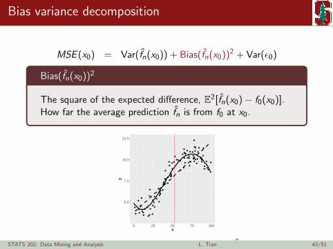
Bias variance decomposition
MSE (x0) = Var(fn(x0)) + Bias(fn(x0))2 + Var(ε0)
Bias(fn(x0))2
The square of the expected difference, E2[fn(x0)− f0(x0)].How far the average prediction fn is from f0 at x0.
●
●
●
●
●
●
●
●
●
●
●
●
●
●
●
●
●
●
●
●
●
●
●
●
●
●
●
●
●
●
●
●
●
●
●
●
●
●
●
●
●
●
●
●
●
●
●
●
●
●
●
●
●
●
●
●
●
●
●
●
●
●
●
●
●
●
●
●
●
●
●
●
●
●
●
●
●
●
●
●
●
●
●
●
●
●
●
●
●
●
●
●
●
●●
●
●
●
●
●
5.0
7.5
10.0
12.5
0 25 50 75 100x
y
Observed data, true f0, and estimate fn.STATS 202: Data Mining and Analysis L. Tran 43/51
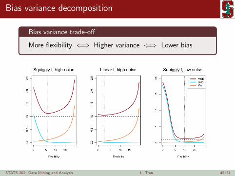
Bias variance decomposition
MSE (x0) = Var(fn(x0)) + Bias(fn(x0))2 + Var(ε0)
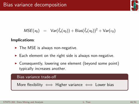
Implications:
I The MSE is always non-negative.
I Each element on the right side is always non-negative.
I Consequently, lowering one element (beyond some point)typically increases another.
Bias variance trade-off
More flexibility ⇐⇒ Higher variance ⇐⇒ Lower bias
STATS 202: Data Mining and Analysis L. Tran 44/51
Bias variance decomposition
Bias variance trade-off
More flexibility ⇐⇒ Higher variance ⇐⇒ Lower bias
STATS 202: Data Mining and Analysis L. Tran 45/51
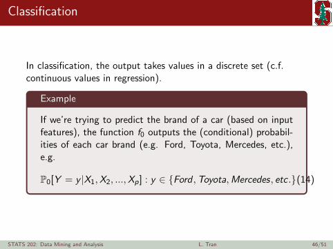
Classification
In classification, the output takes values in a discrete set (c.f.continuous values in regression).
Example
If we’re trying to predict the brand of a car (based on inputfeatures), the function f0 outputs the (conditional) probabil-ities of each car brand (e.g. Ford, Toyota, Mercedes, etc.),e.g.
P0[Y = y |X1,X2, ...,Xp] : y ∈ {Ford ,Toyota,Mercedes, etc .}(14)
STATS 202: Data Mining and Analysis L. Tran 46/51

Comparisons
Regression: f0 = E0[Y |X1,X2, ...,Xp]
I A scalar value, i.e. f0 ∈ R
I fn therefore gives us estimates of y
Classification: f0 = P0[Y = y |X1,X2, ...,Xp]
I A vectored value, i.e.f0 = [p1, p2, ..., pK ] : pj ∈ [0, 1],
∑K pj = 1
I n.b. In a binary setting this simplies to a scalar, i.e.f0 = p1 : p1 = P0[Y = 1|X1,X2, ...,Xp] ∈ [0, 1]
I fn therefore gives us predictions of each class
STATS 202: Data Mining and Analysis L. Tran 47/51

Bayes classifier
I f0 gives us a probability of the observation belonging to eachclass.
I To select a class, we can just pick the element inf0 = [p1, p2, ..., pK ] that’s the largest
I Called the Bayes Classifier
I As a classifier, produces the lowest error rate
Bayes error rate
1− E0
[maxy
P0[Y = y |X1,X2, ...,Xp]
](15)
Analogous to the irreducible error described previously
STATS 202: Data Mining and Analysis L. Tran 48/51
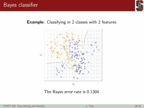
Bayes classifier
Example: Classifying in 2 classes with 2 features.
The Bayes error rate is 0.1304.
STATS 202: Data Mining and Analysis L. Tran 49/51
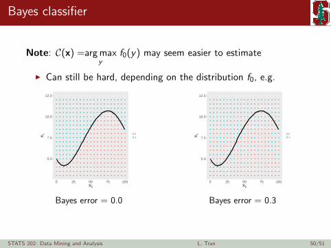
Bayes classifier
Note: C(x) =arg maxy
f0(y) may seem easier to estimate
I Can still be hard, depending on the distribution f0, e.g.
● ● ● ● ● ● ● ● ● ● ● ● ● ● ● ● ● ● ● ● ●
● ● ● ● ● ● ● ● ● ● ● ● ● ● ● ● ● ● ● ● ●
● ● ● ● ● ● ● ● ● ● ● ● ● ● ● ● ● ● ● ● ●
● ● ● ● ● ● ● ● ● ● ● ● ● ● ● ● ● ●
● ● ● ● ● ● ● ● ● ● ● ● ● ● ● ●
● ● ● ● ● ● ● ● ● ● ● ● ● ● ●
● ● ● ● ● ● ● ● ● ● ● ● ● ●
● ● ● ● ● ● ● ● ● ● ● ● ● ●
● ● ● ● ● ● ● ● ● ● ● ● ●
● ● ● ● ● ● ● ● ● ● ● ●
● ● ● ● ● ● ● ● ● ● ● ●
● ● ● ● ● ● ● ● ● ●
● ● ● ● ● ● ● ● ●
● ● ● ● ● ● ●
● ● ● ● ●
● ● ●
5.0
7.5
10.0
12.5
0 25 50 75 100X2
X1 ● 0
1
Bayes error = 0.0
● ● ● ● ● ● ● ● ● ● ● ● ● ● ● ●
● ● ● ● ● ● ● ● ● ● ● ● ● ● ● ●
● ● ● ● ● ● ● ● ● ● ● ● ● ● ●
● ● ● ● ● ● ● ● ● ● ● ● ● ●
● ● ● ● ● ● ● ● ● ● ● ● ● ● ●
● ● ● ● ● ● ● ● ● ● ●
● ● ● ● ● ● ● ● ● ● ● ● ● ● ●
● ● ● ● ● ● ● ● ● ● ● ● ● ●
● ● ● ● ● ● ● ● ● ● ● ● ● ●
● ● ● ● ● ● ● ● ● ● ●
● ● ● ● ● ● ● ● ● ● ● ● ●
● ● ● ● ● ● ● ● ● ● ● ● ● ●
● ● ● ● ● ● ● ●
● ● ● ● ● ● ● ● ● ● ● ●
● ● ● ● ●
● ● ● ● ● ●
● ● ● ● ● ● ● ● ●
● ● ● ● ● ● ● ● ●
● ● ● ● ● ● ●
5.0
7.5
10.0
12.5
0 25 50 75 100X2
X1 ● 0
1
Bayes error = 0.3
STATS 202: Data Mining and Analysis L. Tran 50/51
References
[1] ISL. Chapters 1-2.
[2] ESL. Chapters 1-2.
STATS 202: Data Mining and Analysis L. Tran 51/51