Syllabus Introduction Trend vs. Cycle Facts Model

Lecture 1: Introduction

Advanced MacroeconomicsUniversity of Warsaw

Jacek Suda

March 1, 2017

Lecture 1

Syllabus Introduction Trend vs. Cycle Facts Model

Plan of the Presentation

1 Syllabus

2 Introduction

3 Trend vs. Cycle

4 Business Cycle Facts

5 DSGE models

Lecture 1

Syllabus Introduction Trend vs. Cycle Facts Model Requirements Readings

Website

Class website: http://www.jaceksuda.com/teach/

Email: jacek.suda@gmail.com

Lecture 1

Syllabus Introduction Trend vs. Cycle Facts Model Requirements Readings

Description

The main objective of the course is to introduce fundamental techniquesfor constructing and solving dynamic-stochastic general equilibrium (DSGE)models.

We begin with the basic growth/RBC (Real Business Cycle) model. Themodel (and its extension) will be used to illustrate the concept of equi-librium, market completeness, and solution techniques.We will also use it to show some properties of the business cycles as wellas its implications for asset prices and macroeconomic policy.

The second part of the course introduces the overlapping generation(OLG) model and, if time permits, incomplete markets model (agentsface idiosyncratic and uninsurable labor income risk).

Lecture 1

Syllabus Introduction Trend vs. Cycle Facts Model Requirements Readings

Requirements

Three homework assignment with the weight of 30% of final grade.

The class ends either in-class 2 hour long exam or take-home exam.

Lecture 1

Syllabus Introduction Trend vs. Cycle Facts Model Requirements Readings

Readings

No single textbook but a number of textbooks covers a part of materialdiscussed in class

Frontiers of Business Cycle Research by Thomas Cooley, PrincetonUniversity Press, 1995.Recursive Macroeconomic Theory by Lars Ljungqvist and ThomasSargent, Princeton University Press, 2010.The ABCs of RBCs: An Intoduction to Dynamic Macroeconomic Modelsby Geroge McCandless, Harvard University Press, 2008.

Other texts areDynamic Economics by Jerome Adda and Russel Cooper, MIT Press,2003.Structural Macroeconometrics by David N. DeJong with Chetan Dave,Princeton University Press, 2007.Advanced Macroeconomics by David Romer, McGraw Hill, 1996.Recursive Methods in Economic Dynamics by Nancy Stokey and RobertLucas with Edward Prescott, Harvard University Press, 1989.

Lecture 1

Syllabus Introduction Trend vs. Cycle Facts Model

Plan of the Presentation

1 Syllabus

2 Introduction

3 Trend vs. Cycle

4 Business Cycle Facts

5 DSGE models

Lecture 1

Syllabus Introduction Trend vs. Cycle Facts Model

Lucas critique

Until the 1970s macroeconomic modeling was dominated bylarge-scale models (Cowles Commission approach)These models consisted of estimated ad-hoc equations, e.g. the Phillipscurve, and lacked cross-equations restrinctionsThis approach was criticized by Lucas (1976) (Lucas critique)

ad-hoc equation parameters are sensitive to policy modifications ⇒ only,,deep” parameters should be usedexpectations crucial in driving agent’s decisions

Lecture 1

Syllabus Introduction Trend vs. Cycle Facts Model

RBC as DSGE

The general equilibrium (GE) approach to modeling was a response tothe Lucas critiqueThe RBC model (Kydland and Prescott, 1982) are derived frommicrofoundations:

households solves intertemporal (dynamic) problem (maximize utility)firms maximize profitsthey take into account policy changes

RBC models form the basis of modern macroeconomic modelingFurther advances in DSGE modeling build on the RBC frameworkCaveat: it a simple model:

simple RBC models explain the business cycle as coming solely fromproductivity shocks⇒ no role for empirically valid demand shocks (e.g. monetary policy)

Lecture 1

Syllabus Introduction Trend vs. Cycle Facts Model

Plan of the Presentation

1 Syllabus

2 Introduction

3 Trend vs. Cycle

4 Business Cycle Facts

5 DSGE models

Lecture 1

Syllabus Introduction Trend vs. Cycle Facts Model

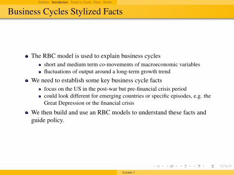
Business Cycles Stylized Facts

The RBC model is used to explain business cyclesshort and medium term co-movements of macroeconomic variablesfluctuations of output around a long-term growth trend

We need to establish some key business cycle factsfocus on the US in the post-war but pre-financial crisis periodcould look different for emerging countries or specific episodes, e.g. theGreat Depression or the financial crisis

We then build and use an RBC models to understand these facts andguide policy.

Lecture 1

Syllabus Introduction Trend vs. Cycle Facts Model

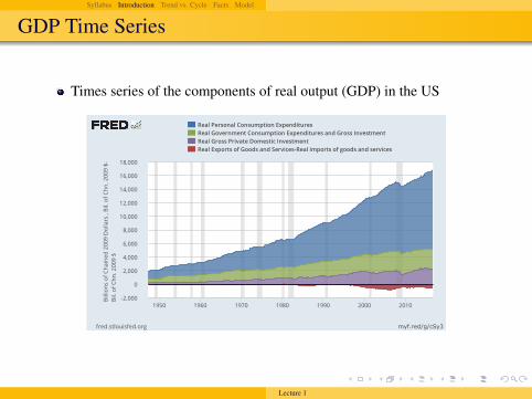
GDP Time Series

Times series of real output (GDP) in the US

myf.red/g/cSxV

0

2,000

4,000

6,000

8,000

10,000

12,000

14,000

16,000

18,000

1950 1960 1970 1980 1990 2000 2010

fred.stlouisfed.orgSource:U.S.BureauofEconomicAnalysis

RealGrossDomesticProduct

BillionsofChained2009Dollars

Lecture 1

Syllabus Introduction Trend vs. Cycle Facts Model

GDP Time Series

Times series of real output (GDP) in the US, log scale

myf.red/g/cSxX

2,400

2,800

3,200

4,000

6,000

8,000

10,000

12,000

14,000

16,00018,000

1950 1960 1970 1980 1990 2000 2010

fred.stlouisfed.orgSource:U.S.BureauofEconomicAnalysis

RealGrossDomesticProduct

BillionsofC

hained2009Dollars

Lecture 1

Syllabus Introduction Trend vs. Cycle Facts Model

GDP Time Series

Times series of the growth of real output (GDP) in the US

myf.red/g/cSy0

-15

-10

-5

0

5

10

15

20

1950 1960 1970 1980 1990 2000 2010

fred.stlouisfed.orgSource:U.S.BureauofEconomicAnalysis

RealGrossDomesticProduct

PercentChangefrom

PrecedingPeriod

Lecture 1

Syllabus Introduction Trend vs. Cycle Facts Model

GDP Time Series

Times series of the components of real output (GDP) in the US

myf.red/g/cSy3

-2,000

0

2,000

4,000

6,000

8,000

10,000

12,000

14,000

16,000

18,000

1950 1960 1970 1980 1990 2000 2010

fred.stlouisfed.org

RealPersonalConsumptionExpendituresRealGovernmentConsumptionExpendituresandGrossInvestmentRealGrossPrivateDomesticInvestmentRealExportsofGoodsandServices-Realimportsofgoodsandservices

BillionsofC

hained

2009Dollars,Bil.ofC

hn.2009$-

Bil.ofC

hn.2009$

Lecture 1

Syllabus Introduction Trend vs. Cycle Facts Model

GDP/Output

Output has grown on average, butat variable ratefluctuated around some trend

Recessions and expansions differed in size, length, frequencyGrowth rate of GDP

varies over timefeatures changing over time volatility

How to separate the cycle (fluctuations around) from the trend?

Lecture 1

Syllabus Introduction Trend vs. Cycle Facts Model

Plan of the Presentation

1 Syllabus

2 Introduction

3 Trend vs. Cycle

4 Business Cycle Facts

5 DSGE models

Lecture 1

Syllabus Introduction Trend vs. Cycle Facts Model

Detrending data

Several methods for detrending (filtering) the dataMost popular filters:

Linear trendHP (Hodrick-Prescott) filterBandpass filter

Lecture 1

Syllabus Introduction Trend vs. Cycle Facts Model

Trend and Cycle

Denote log of actual GDP (or any other variable of interest) as yt

yt = log GDP

Let yt be the trend (or growth) component of yt

Let yt be cyclical (or detrended) component of yt

yt ≡ yt − yt

Sometimes trend is viewed as “potential” GDP

Lecture 1

Syllabus Introduction Trend vs. Cycle Facts Model

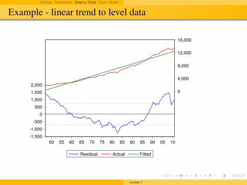
Linear trend

Define linear trend asyt ≡ g · t

where g is the average growth rateUntil the late 70s:

fit a linear trend: yt is the residual of regressing yt on t.define the stochastic part of the time series as deviations from this trend

Conceptually simple but not that useful if low-frequency movementsare different than exact deterministic linear trend (e.g., demographics,secular stagnation)Example: problem in late 70s:

The “trend” (potential) GDP growth rate slowed down

Lecture 1

Syllabus Introduction Trend vs. Cycle Facts Model

HP Filter

Hodrick-Prescott filter: define trend as the solution to minimization ofthe loss function:

L =∑

t

(yt − yt)2 + λ

∑t

((yt+1 − yt)− (yt − yt−1))2

λ is the parameter that governs the punishment for the variations in thegrowth component

Trend converges to a linear trend when λ → ∞Trend converges to actual data as λ → 0

Standard value for λ for quarterly data is λ = 1600Ravn and Uhlig (2002) suggests that λ should equal the fourth power ofthe frequency observation ratio

Hamilton (2017) suggests we should never use HP filter:

“A regression of the variable at date t + h on the four most re-cent values as of date t offers a robust approach to detrending thatachieves all the objectives sought by users of the HP filter with noneof its drawbacks.”

Lecture 1

Syllabus Introduction Trend vs. Cycle Facts Model

Example - linear trend to level data

-1,500

-1,000

-500

0

500

1,000

1,500

2,000

0

4,000

8,000

12,000

16,000

50 55 60 65 70 75 80 85 90 95 00 05 10

Residual Actual Fitted

Lecture 1

Syllabus Introduction Trend vs. Cycle Facts Model

Example - HP trend to log data

-.08

-.06

-.04

-.02

.00

.02

.04

7.2

7.6

8.0

8.4

8.8

9.2

9.6

50 55 60 65 70 75 80 85 90 95 00 05 10

LOG_GDP Trend Cycle

Hodrick-Prescott Filter (lambda=1600)

Lecture 1

Syllabus Introduction Trend vs. Cycle Facts Model

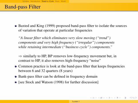
Band-pass Filter

Baxted and King (1999) proposed band-pass filter to isolate the sourcesof variation that operate at particular frequencies

“A linear filter which eliminates very slow moving (“trend”)components and very high frequency (“irregular”) componentswhile retaining intermediate (“business cycle”) components.”

⇒ similarly to HP, BP removes low-frequency movement but, incontrast to HP, it also removes high-frequency “noise”Common practice is look at the band-pass filter that keeps frequenciesbetween 6 and 32 quarters (8 years)Bank-pass filter can be defined in frequency domain[see Stock and Watson (1998) for further discussion]

Lecture 1

Syllabus Introduction Trend vs. Cycle Facts Model

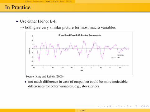
In Practice

Use either H-P or B-P:→ both give very similar picture for most macro variables

Introduction Cycle vs. Trend Business Cycle Facts Conclusion

In Practice• the next figure illustrates the similarity of the cyclical componentsof GDP that we obtain if we apply either the HP or the BP filter.

)LJXUH 4

2XWSXW DQG +3 7UHQG

:15

:17

:19

:1;

;

;15

;17

;19

;1;

7: 85 8: 95 9: :5 :: ;5 ;: <5

'DWH

/RJDULWKP

2XWSXW+3 7UHQG

+3 DQG %DQG 3DVV +9/65, &\FOLFDO &RPSRQHQWV

0;

09

07

05

3

5

7

9

7: 85 8: 95 9: :5 :: ;5 ;: <5

'DWH

3HUFHQW

%3+9/65,+3

+3 *URZWK &RPSRQHQW DQG /LQHDU 7UHQG 5HVLGXDO

048

043

08

3

8

43

48

7: 85 8: 95 9: :5 :: ;5 ;: <5

'DWH

3HUFHQW

2XWSXW OHVV /LQHDU 7UHQG+3 7UHQG OHVV /LQHDU 7UHQG

1RWH= 6DPSOH SHULRG LV 4<7:=4 0 4<<9=71

• clearly, there isn’t much difference in the case of output. note,however, that there could be more noticeable differences for othervariables. think, e.g., of stock prices.

Source: King and Rebelo (2000)

not much difference in case of output but could be more noticeabledifferences for other variables, e.g., stock prices

Lecture 1

Syllabus Introduction Trend vs. Cycle Facts Model

In Practice

Use either H-P or B-P:→ both give very similar picture for most macro variables

Alternative: look at the cyclical properties of the changes (growth rates)

yt ≡ yt − yt−1

But ‘first differences” gives too much emphasis on very short-livedmovements (“noise”)

to some extent the HP filter also keeps this noise while band-pass filterremoves it.

Lecture 1

Syllabus Introduction Trend vs. Cycle Facts Model

In Practice: trend matters matters for cycle

Use the HP filter with caution, especially around large shocks: they candistort estimates of the underlying trends, both before and after theshockJames Bullard, “Housing in America: Innovative Solutions to Addressthe Needs of Tomorrow ”, 5 June 2012

Bullard (2012)

Lecture 1

Syllabus Introduction Trend vs. Cycle Facts Model

Plan of the Presentation

1 Syllabus

2 Introduction

3 Trend vs. Cycle

4 Business Cycle Facts

5 DSGE models

Lecture 1

Syllabus Introduction Trend vs. Cycle Facts Model

Business Cycle Facts

We report facts from King and Rebelo (2000)King and Rebello (2000) use the HP filter and concentrate on realquantitiesStock and Watson (1998) use BP filter

As RBC is concerned exclusively with real quantities we abstact fornow from nominal variables

See Stock and Watson (1998) for a more detailed discussion of all thekey business cycle facts

Lecture 1

Syllabus Introduction Trend vs. Cycle Facts Model

ConsumptionIntroduction Cycle vs. Trend Business Cycle Facts Conclusion

Consumption)LJXUH 5

1RQGXUDEOHV &RQVXPSWLRQ DQG 2XWSXW

0;

09

07

05

3

5

7

9

7: 85 8: 95 9: :5 :: ;5 ;: <5'DWH

3HUFHQW

2XWSXW&RQVXPSWLRQ +1',

'XUDEOHV &RQVXPSWLRQ DQG 2XWSXW

053

048

043

08

3

8

43

48

53

58

63

7: 85 8: 95 9: :5 :: ;5 ;: <5'DWH

3HUFHQW

2XWSXW&RQVXPSWLRQ +',

,QYHVWPHQW DQG 2XWSXW

053

048

043

08

3

8

43

48

7: 85 8: 95 9: :5 :: ;5 ;: <5

'DWH

3HUFHQW

2XWSXW,QYHVWPHQW

*RYHUQPHQW 6SHQGLQJ DQG 2XWSXW

058

053

048

043

08

3

8

43

48

7: 85 8: 95 9: :5 :: ;5 ;: <5

'DWH

3HUFHQW

2XWSXW*RY*W 6SHQGLQJ

1RWH= 6DPSOH SHULRG LV 4<7:=4 0 4<<9=71 $OO YDULDEOHV DUH GHWUHQGHG XVLQJ WKH +RGULFN03UHVFRWW ILOWHU1

Introduction Cycle vs. Trend Business Cycle Facts Conclusion

Consumption)LJXUH 5

1RQGXUDEOHV &RQVXPSWLRQ DQG 2XWSXW

0;

09

07

05

3

5

7

9

7: 85 8: 95 9: :5 :: ;5 ;: <5'DWH

3HUFHQW

2XWSXW&RQVXPSWLRQ +1',

'XUDEOHV &RQVXPSWLRQ DQG 2XWSXW

053

048

043

08

3

8

43

48

53

58

63

7: 85 8: 95 9: :5 :: ;5 ;: <5'DWH

3HUFHQW

2XWSXW&RQVXPSWLRQ +',

,QYHVWPHQW DQG 2XWSXW

053

048

043

08

3

8

43

48

7: 85 8: 95 9: :5 :: ;5 ;: <5

'DWH

3HUFHQW

2XWSXW,QYHVWPHQW

*RYHUQPHQW 6SHQGLQJ DQG 2XWSXW

058

053

048

043

08

3

8

43

48

7: 85 8: 95 9: :5 :: ;5 ;: <5

'DWH

3HUFHQW

2XWSXW*RY*W 6SHQGLQJ

1RWH= 6DPSOH SHULRG LV 4<7:=4 0 4<<9=71 $OO YDULDEOHV DUH GHWUHQGHG XVLQJ WKH +RGULFN03UHVFRWW ILOWHU1

Source: King and Rebelo (2000)

Lecture 1

Syllabus Introduction Trend vs. Cycle Facts Model

Consumption

Consumption is positively correlated with output (pro-cyclical)

Spending on durables is more volatile than output

Spending on non-durables is less volatile than output

Lecture 1

Syllabus Introduction Trend vs. Cycle Facts Model

Investment

Investment is strongly pro-cyclical and more volatile than output

Introduction Cycle vs. Trend Business Cycle Facts Conclusion

Investment

• Investment is strongly pro-cyclical and more volatile than output

)LJXUH 5

1RQGXUDEOHV &RQVXPSWLRQ DQG 2XWSXW

0;

09

07

05

3

5

7

9

7: 85 8: 95 9: :5 :: ;5 ;: <5'DWH

3HUFHQW

2XWSXW&RQVXPSWLRQ +1',

'XUDEOHV &RQVXPSWLRQ DQG 2XWSXW

053

048

043

08

3

8

43

48

53

58

63

7: 85 8: 95 9: :5 :: ;5 ;: <5'DWH

3HUFHQW

2XWSXW&RQVXPSWLRQ +',

,QYHVWPHQW DQG 2XWSXW

053

048

043

08

3

8

43

48

7: 85 8: 95 9: :5 :: ;5 ;: <5

'DWH

3HUFHQW

2XWSXW,QYHVWPHQW

*RYHUQPHQW 6SHQGLQJ DQG 2XWSXW

058

053

048

043

08

3

8

43

48

7: 85 8: 95 9: :5 :: ;5 ;: <5

'DWH

3HUFHQW

2XWSXW*RY*W 6SHQGLQJ

1RWH= 6DPSOH SHULRG LV 4<7:=4 0 4<<9=71 $OO YDULDEOHV DUH GHWUHQGHG XVLQJ WKH +RGULFN03UHVFRWW ILOWHU1

Source: King and Rebelo (2000)

Lecture 1

Syllabus Introduction Trend vs. Cycle Facts Model

Labor

The labor input (total hours) is pro-cyclical and as volatile as output

Introduction Cycle vs. Trend Business Cycle Facts Conclusion

Labor

• The labor input (total hours) is pro-cyclical and as volatile as output)LJXUH 6

7RWDO +RXUV DQG 2XWSXW

0;

09

07

05

3

5

7

9

7: 85 8: 95 9: :5 :: ;5 ;: <5'DWH

3HUFHQW

2XWSXW7RWDO +RXUV

&DSLWDO DQG 2XWSXW

0;

09

07

05

3

5

7

9

7: 85 8: 95 9: :5 :: ;5 ;: <5'DWH

3HUFHQW

2XWSXW&DSLWDO

&DSLWDO 8WLOL]DWLRQ DQG 2XWSXW

048

043

08

3

8

43

7: 85 8: 95 9: :5 :: ;5 ;: <5'DWH

3HUFHQW

2XWSXW&DSLWDO 8WLOL]DWLRQ

3URGXFWLYLW\ +6RORZ UHVLGXDO, DQG 2XWSXW

0;

09

07

05

3

5

7

9

7: 85 8: 95 9: :5 :: ;5 ;: <5'DWH

3HUFHQW

2XWSXW3URGXFWLYLW\

1RWH= 6DPSOH SHULRG LV 4<7:=4 0 4<<9=71 $OO YDULDEOHV DUH GHWUHQGHG XVLQJ WKH +RGULFN03UHVFRWW ILOWHU1

Source: King and Rebelo (2000)

Lecture 1

Syllabus Introduction Trend vs. Cycle Facts Model

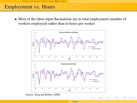
Employment vs. Hours

Most of the labor-input fluctuations are in total employment (number ofworkers employed) rather than in hours per worker

Introduction Cycle vs. Trend Business Cycle Facts Conclusion

Employment vs. Hours• Most of the labor-input fluctuations are in total employment(number of workers employed) rather than in hours per worker)LJXUH 7

+RXUV SHU :RUNHU DQG 2XWSXW

0;

09

07

05

3

5

7

9

7: 85 8: 95 9: :5 :: ;5 ;: <5

'DWH

3HUFHQW

2XWSXW+RXUV SHU :RUNHU

(PSOR\PHQW DQG 2XSXW

0;

09

07

05

3

5

7

9

7: 85 8: 95 9: :5 :: ;5 ;: <5

'DWH

3HUFHQW

2XWSXW(PSOR\PHQW

$YHUDJH 3URGXFW DQG 2XWSXW

0;

09

07

05

3

5

7

9

7: 85 8: 95 9: :5 :: ;5 ;: <5

'DWH

3HUFHQW

2XWSXW$YHUDJH 3URGXFW

5HDO :DJHV DQG 2XWSXW

0;

09

07

05

3

5

7

9

7: 85 8: 95 9: :5 :: ;5 ;: <5

'DWH

3HUFHQW

2XWSXW5HDO :DJHV

1RWH= 6DPSOH SHULRG LV 4<7:=4 0 4<<9=71 $OO YDULDEOHV DUH GHWUHQGHG XVLQJ WKH +RGULFN03UHVFRWW ILOWHU1

Introduction Cycle vs. Trend Business Cycle Facts Conclusion

Employment vs. Hours• Most of the labor-input fluctuations are in total employment(number of workers employed) rather than in hours per worker)LJXUH 7

+RXUV SHU :RUNHU DQG 2XWSXW

0;

09

07

05

3

5

7

9

7: 85 8: 95 9: :5 :: ;5 ;: <5

'DWH

3HUFHQW

2XWSXW+RXUV SHU :RUNHU

(PSOR\PHQW DQG 2XSXW

0;

09

07

05

3

5

7

9

7: 85 8: 95 9: :5 :: ;5 ;: <5

'DWH

3HUFHQW

2XWSXW(PSOR\PHQW

$YHUDJH 3URGXFW DQG 2XWSXW

0;

09

07

05

3

5

7

9

7: 85 8: 95 9: :5 :: ;5 ;: <5

'DWH

3HUFHQW

2XWSXW$YHUDJH 3URGXFW

5HDO :DJHV DQG 2XWSXW

0;

09

07

05

3

5

7

9

7: 85 8: 95 9: :5 :: ;5 ;: <5

'DWH

3HUFHQW

2XWSXW5HDO :DJHV

1RWH= 6DPSOH SHULRG LV 4<7:=4 0 4<<9=71 $OO YDULDEOHV DUH GHWUHQGHG XVLQJ WKH +RGULFN03UHVFRWW ILOWHU1

Source: King and Rebelo (2000)

Lecture 1

Syllabus Introduction Trend vs. Cycle Facts Model

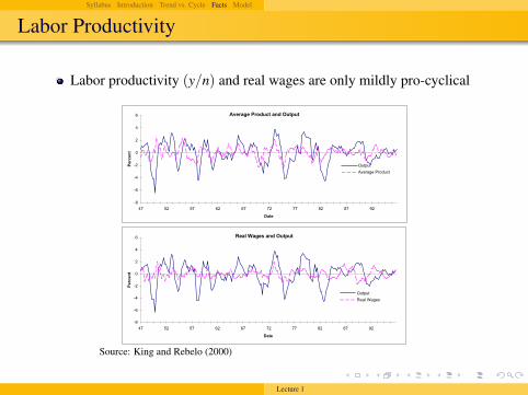
Labor Productivity

Labor productivity (y/n) and real wages are only mildly pro-cyclical

Introduction Cycle vs. Trend Business Cycle Facts Conclusion

Labor Productivity• Labor productivity (y/n) and real wages are only mildly procyclical

)LJXUH 7

+RXUV SHU :RUNHU DQG 2XWSXW

0;

09

07

05

3

5

7

9

7: 85 8: 95 9: :5 :: ;5 ;: <5

'DWH

3HUFHQW

2XWSXW+RXUV SHU :RUNHU

(PSOR\PHQW DQG 2XSXW

0;

09

07

05

3

5

7

9

7: 85 8: 95 9: :5 :: ;5 ;: <5

'DWH

3HUFHQW

2XWSXW(PSOR\PHQW

$YHUDJH 3URGXFW DQG 2XWSXW

0;

09

07

05

3

5

7

9

7: 85 8: 95 9: :5 :: ;5 ;: <5

'DWH

3HUFHQW

2XWSXW$YHUDJH 3URGXFW

5HDO :DJHV DQG 2XWSXW

0;

09

07

05

3

5

7

9

7: 85 8: 95 9: :5 :: ;5 ;: <5

'DWH

3HUFHQW

2XWSXW5HDO :DJHV

1RWH= 6DPSOH SHULRG LV 4<7:=4 0 4<<9=71 $OO YDULDEOHV DUH GHWUHQGHG XVLQJ WKH +RGULFN03UHVFRWW ILOWHU1

Introduction Cycle vs. Trend Business Cycle Facts Conclusion

Labor Productivity• Labor productivity (y/n) and real wages are only mildly procyclical

)LJXUH 7

+RXUV SHU :RUNHU DQG 2XWSXW

0;

09

07

05

3

5

7

9

7: 85 8: 95 9: :5 :: ;5 ;: <5

'DWH

3HUFHQW

2XWSXW+RXUV SHU :RUNHU

(PSOR\PHQW DQG 2XSXW

0;

09

07

05

3

5

7

9

7: 85 8: 95 9: :5 :: ;5 ;: <5

'DWH

3HUFHQW

2XWSXW(PSOR\PHQW

$YHUDJH 3URGXFW DQG 2XWSXW

0;

09

07

05

3

5

7

9

7: 85 8: 95 9: :5 :: ;5 ;: <5

'DWH

3HUFHQW

2XWSXW$YHUDJH 3URGXFW

5HDO :DJHV DQG 2XWSXW

0;

09

07

05

3

5

7

9

7: 85 8: 95 9: :5 :: ;5 ;: <5

'DWH

3HUFHQW

2XWSXW5HDO :DJHV

1RWH= 6DPSOH SHULRG LV 4<7:=4 0 4<<9=71 $OO YDULDEOHV DUH GHWUHQGHG XVLQJ WKH +RGULFN03UHVFRWW ILOWHU1

Source: King and Rebelo (2000)

Lecture 1

Syllabus Introduction Trend vs. Cycle Facts Model

Capital

The capital stock moves very slowlyCapital utilization is highly pro-cyclical⇒ effective capital input is highly pro-cyclical

Introduction Cycle vs. Trend Business Cycle Facts Conclusion

Capital• The capital stock moves very slowly, but capital utilization is highlyprocyclical, so that effective capital input is highly pro-cyclical

)LJXUH 6

7RWDO +RXUV DQG 2XWSXW

0;

09

07

05

3

5

7

9

7: 85 8: 95 9: :5 :: ;5 ;: <5'DWH

3HUFHQW

2XWSXW7RWDO +RXUV

&DSLWDO DQG 2XWSXW

0;

09

07

05

3

5

7

9

7: 85 8: 95 9: :5 :: ;5 ;: <5'DWH

3HUFHQW

2XWSXW&DSLWDO

&DSLWDO 8WLOL]DWLRQ DQG 2XWSXW

048

043

08

3

8

43

7: 85 8: 95 9: :5 :: ;5 ;: <5'DWH

3HUFHQW

2XWSXW&DSLWDO 8WLOL]DWLRQ

3URGXFWLYLW\ +6RORZ UHVLGXDO, DQG 2XWSXW

0;

09

07

05

3

5

7

9

7: 85 8: 95 9: :5 :: ;5 ;: <5'DWH

3HUFHQW

2XWSXW3URGXFWLYLW\

1RWH= 6DPSOH SHULRG LV 4<7:=4 0 4<<9=71 $OO YDULDEOHV DUH GHWUHQGHG XVLQJ WKH +RGULFN03UHVFRWW ILOWHU1

Introduction Cycle vs. Trend Business Cycle Facts Conclusion

Capital• The capital stock moves very slowly, but capital utilization is highlyprocyclical, so that effective capital input is highly pro-cyclical

)LJXUH 6

7RWDO +RXUV DQG 2XWSXW

0;

09

07

05

3

5

7

9

7: 85 8: 95 9: :5 :: ;5 ;: <5'DWH

3HUFHQW

2XWSXW7RWDO +RXUV

&DSLWDO DQG 2XWSXW

0;

09

07

05

3

5

7

9

7: 85 8: 95 9: :5 :: ;5 ;: <5'DWH

3HUFHQW

2XWSXW&DSLWDO

&DSLWDO 8WLOL]DWLRQ DQG 2XWSXW

048

043

08

3

8

43

7: 85 8: 95 9: :5 :: ;5 ;: <5'DWH

3HUFHQW

2XWSXW&DSLWDO 8WLOL]DWLRQ

3URGXFWLYLW\ +6RORZ UHVLGXDO, DQG 2XWSXW

0;

09

07

05

3

5

7

9

7: 85 8: 95 9: :5 :: ;5 ;: <5'DWH

3HUFHQW

2XWSXW3URGXFWLYLW\

1RWH= 6DPSOH SHULRG LV 4<7:=4 0 4<<9=71 $OO YDULDEOHV DUH GHWUHQGHG XVLQJ WKH +RGULFN03UHVFRWW ILOWHU1

Source: King and Rebelo (2000)

Lecture 1

Syllabus Introduction Trend vs. Cycle Facts Model

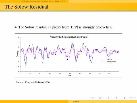
The Solow Residual

The Solow residual (a proxy from TFP) is strongly procyclical

Introduction Cycle vs. Trend Business Cycle Facts Conclusion

The Solow Residual

• The Solow residual (a proxy from TFP) is strongly procyclical

)LJXUH 6

7RWDO +RXUV DQG 2XWSXW

0;

09

07

05

3

5

7

9

7: 85 8: 95 9: :5 :: ;5 ;: <5'DWH

3HUFHQW

2XWSXW7RWDO +RXUV

&DSLWDO DQG 2XWSXW

0;

09

07

05

3

5

7

9

7: 85 8: 95 9: :5 :: ;5 ;: <5'DWH

3HUFHQW

2XWSXW&DSLWDO

&DSLWDO 8WLOL]DWLRQ DQG 2XWSXW

048

043

08

3

8

43

7: 85 8: 95 9: :5 :: ;5 ;: <5'DWH

3HUFHQW

2XWSXW&DSLWDO 8WLOL]DWLRQ

3URGXFWLYLW\ +6RORZ UHVLGXDO, DQG 2XWSXW

0;

09

07

05

3

5

7

9

7: 85 8: 95 9: :5 :: ;5 ;: <5'DWH

3HUFHQW

2XWSXW3URGXFWLYLW\

1RWH= 6DPSOH SHULRG LV 4<7:=4 0 4<<9=71 $OO YDULDEOHV DUH GHWUHQGHG XVLQJ WKH +RGULFN03UHVFRWW ILOWHU1

Source: King and Rebelo (2000)

Lecture 1

Syllabus Introduction Trend vs. Cycle Facts Model

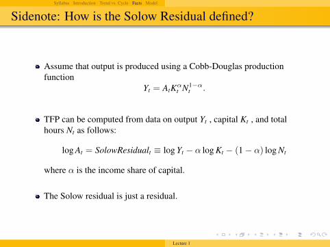
Sidenote: How is the Solow Residual defined?

Assume that output is produced using a Cobb-Douglas productionfunction

Yt = AtKαt N1−α

t .

TFP can be computed from data on output Yt , capital Kt , and totalhours Nt as follows:

log At = SolowResidualt ≡ log Yt − α log Kt − (1− α) log Nt

where α is the income share of capital.

The Solow residual is just a residual.

Lecture 1

Syllabus Introduction Trend vs. Cycle Facts Model

Variances and Co-variances

Basic business-cycle statistics for the US economy from King andRebelo (2000).(all variables expect for the interest rate are HP filtered)

Introduction Cycle vs. Trend Business Cycle Facts Conclusion

Variances and Co-variances

• Basic business-cycle statistics for the US economyfrom King and Rebelo (2000).

-" ◆⌦◆ :⇧8⌧ ⇧8=⇧ ⌧*(85� �-((*�598-1 8⌧ 9⇧* (*5⌧-1 ⌫⇧� 9⇧*(* 8⌧ ⌧-⇤* �(*;8�9508�89�9- 9⇧* 0�⌧81*⌧⌧ ����*◆

:50�* ⌅�⌧81*⌧⌧ '���* ⌃9598⌧98�⌧ "-( 9⇧* 3◆⌃◆ %�-1-⇤�

⌃951;5(;)*48598-1

!*�5984*⌃951;5(;)*48598-1

⇣8(⌧9<(;*(✓�9-⌥�-((*�598-1

'-19*⇤�-(51*-�⌧'-((*�598-1⌫89⇧<�9��9

& ◆� ◆ ◆�⇢ ◆ ' ◆,� ◆+⇢ ◆� ◆��� �◆, 7◆⌦, ◆�+ ◆� ↵ ◆+⌦ ◆⌦⌦ ◆�� ◆��&.↵ ◆ 7 ◆� ◆+⇢ ◆��⌫ ◆ � ◆,� ◆ ◆7( ◆, ◆ ◆ ⌥ ◆,�✓ ◆⌦� ◆�⇢ ◆+⇢ ◆+�

↵-9*⇠ ✓�� 45(850�*⌧ 5(* 81 �-=5(89⇧⇤⌧ ✏⌫89⇧ 9⇧* *��*�98-1 -" 9⇧*(*5� 819*(*⌧9 (59*/ 51; ⇧54* 0**1 ;*9(*1;*; ⌫89⇧ 9⇧* 6# ��9*(◆ )595⌧-�(�*⌧ 5(* ;*⌧�(80*; 81 ⌃9-�$ 51; >59⌧-1 �⌦⌦�⇥⌘ ⌫⇧- �(*59*; 9⇧*(*5� (59* �⌧81= ⇡✓! 812598-1 *��*�9598-1⌧◆ <�( 1-9598-1 81 9⇧8⌧ 950�*�-((*⌧�-1;⌧ 9- 9⇧59 81 9⇧* 9*�9⌘ ⌧- 9⇧59 & 8⌧ �*( �5�895 -�9��9⌘ ' 8⌧ �*(�5�895 �-1⌧�⇤�98-1⌘ � 8⌧ �*( �5�895 814*⌧9⇤*19⌘ ↵ 8⌧ �*( �5�895 ⇧-�(⌧⌘⌫ 8⌧ 9⇧* (*5� ⌫5=* ✏�-⇤�*1⌧598-1 �*( ⇧-�(/⌘ ( 8⌧ 9⇧* (*5� 819*(*⌧9 (59*⌘51; ✓ 8⌧ 9-95� "5�9-( �(-;��98489�◆

�1 �(*⌧*1981= 9⇧*⌧* 0�⌧81*⌧⌧ ����* "5�9⌧⌘ ⌫* 5(* "-��⌧81= -1 5 ⌧⇤5�� 1�⇤0*(-" *⇤�8(8�5� "*59�(*⌧ 9⇧59 ⇧54* 0**1 *�9*1⌧84*�� ;8⌧��⌧⌧*; 81 (*�*19 ⌫-($ -1 (*5�0�⌧81*⌧⌧ ����*⌧◆ ⇣-( *�5⇤��*⌘ 81 9⇧* 819*(*⌧9 -" 0(*489�⌘ ⌫* ⇧54* 1-9 ;8⌧��⌧⌧*; 9⇧*�*5;⌥�5= (*�598-1⌧ 0*9⌫**1 -�( 45(850�*⌧◆ �1 �⇧--⌧81= 9⇧* ⌧*(8*⌧ 9- ⌧9�;�⌘ ⌫* ⇧54*5�⌧- �*"9 -�9 1-⇤815� 45(850�*⌧⌘ ⌫⇧-⌧* ����8�5� 0*⇧548-( 8⌧ 59 9⇧* ⇧*5(9 -" ⇤51��-19(-4*(⌧8*⌧ -4*( 9⇧* 159�(* -" 0�⌧81*⌧⌧ ����*⌧◆ 6-⌫*4*(⌘ ⌫* ;- (*�-(9 9⇧*

⌦✓✓ ⌦⌃↵⌧ �⌅� ��⇣⌃⌅ �⇥◆◆⌘⇠ ⇣✓↵⇡⌃⌅⇣ ⇧��✏⇠ ⇧��✏⇠ �⌅� ⌥⇢⇥� �⌃� � �⇡⇣↵⌫⇣⇣⇡⌃⌅ ⌃� �⇡✓��⌫�✓ �⌅�✓⇤ ⇡�⇡↵�� �✓⇣⌫�⇣⇢

⌦

from King and Rebelo (2000)

• all variables except the interest rate are HP filtered

Source: King and Rebelo (2000)

Lecture 1

Syllabus Introduction Trend vs. Cycle Facts Model

Summary

King and Rebelo (2000) reported following business cycle stylizedfacts

Consumption, Investment, and Labor are all strongly pro-cyclical

Durables are more pro-cyclical than non-durables

Employment fluctuates more than hours

Capital moves slowly

Labor productivity and wages are only mildly pro-cyclical

The Solow residual (proxy for TFP) is strongly pro-cyclical

Next step: think about models that may account for these patterns!

Lecture 1

Syllabus Introduction Trend vs. Cycle Facts Model

Plan of the Presentation

1 Syllabus

2 Introduction

3 Trend vs. Cycle

4 Business Cycle Facts

5 DSGE models

Lecture 1

Syllabus Introduction Trend vs. Cycle Facts Model

Plan of the Presentation

1 Syllabus

2 Introduction

3 Trend vs. Cycle

4 Business Cycle Facts

5 DSGE models

Lecture 1

Syllabus Introduction Trend vs. Cycle Facts Model

The problem

DSGE models are derived from microeconomic problemsWrite down the problems

1 households maximize utility s.t. budget constraint2 producers maximize profits s.t. technology3 markets clear

Construct Lagrangeans (or Bellman equations)

Lecture 1

Syllabus Introduction Trend vs. Cycle Facts Model

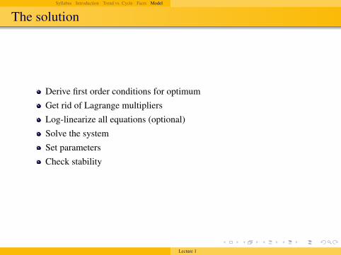
The solution

Derive first order conditions for optimumGet rid of Lagrange multipliersLog-linearize all equations (optional)Solve the systemSet parametersCheck stability

Lecture 1