lecture 1 lsa 2011-for-culearnidiom.ucsd.edu/.../lecture_1_lsa_2011-for-culearn.pdf ·...

Computational Psycholinguistics Lecture 1: Introduction, basic probability theory,

incremental parsing

Florian Jaeger & Roger Levy

LSA 2011 Summer Institute Boulder, CO 8 July 2011

What this class will and will not do

•  We can’t give a comprehensive overview in 8 classes

•  We will try to convey: •  How to profitably combine ideas from computational

linguistics, psycholinguistics, theoretical linguistics, statistics, and cognitive science

•  How these ideas together have led to a productive new view of how language works given incrementality, uncertainty, and noise in the communicative channel

•  We will point out potential research topics when possible

•  We won’t cover work on acquisition (but we do touch on related topics)

Brief instructor self-intros

•  T. Florian Jaeger

•  Roger Levy

Summary of the course: Lecture 1

•  Crash course in probability theory

•  Crash course in natural language syntax and parsing

•  Basic incremental parsing models: Jurafsky 1996


•  Surprisal theory (Hale, 2001; Levy, 2008)

•  Technical foundations: Incremental Earley parsing

•  Applications in syntactic comprehension: •  Garden-pathing

•  Expectation-based facilitation in unambiguous contexts

•  Facilitative ambiguity

•  Digging-in effects and approximate surprisal


•  Zipf’s Principle of Least Effort [Zipf, 1935, 1949]

•  Introduction to information theory [Shannon, 1948]

•  Shannon information •  Entropy (uncertainty) •  Noisy channel •  Noisy Channel theorem

•  Language use, language change and language evolution [Bates and MacWhinney, 1982; Jaeger and Tily, 2011; Nowak et al., 2000, 2001, 2002; Plotkin and Nowak, 2000]

•  Entropy and the mental lexicon [Ferrer i Cancho, XXX; Manin, 2006; Piantadosi et al., 2011; Plotkin and Novak, 2000]

[6]


•  Constant Entropy Rate: Evidence and Critique [Genzel and Charniak, 2002, 2003; Keller, 2004; Moscoso del Prado Martin, 2011; Piantadosi & Gibson, 2008; Qian and Jaeger, 2009, 2010, 2011, submitted]

•  Entropy and alternations (choice points in production)

•  Linking computational level considerations about efficient communication to mechanisms: •  information, probabilities, and activation

[Moscoso del Prado Martin et al. 2006]

•  an activation-based interpretation of constant entropy

[7]


•  Input uncertainty in language processing

•  The Bayesian Reader model of word recognition

•  Noisy-channel sentence comprehension

•  Local-coherence effects

•  Hallucinated garden paths

•  (Modeling eye movement control in reading)


[9]

•  Moving beyond entropy and information density: a model of the ideal speaker

•  Contextual confusability [Lindblom, 1990]

•  Informativity [van Son and Pols, 2003]

•  Resource-bounded production

•  Linking computational level considerations about efficient communication to mechanisms: –  the ‘audience design’ debate in psycholinguistics

[Arnold, 2008; Bard and Aylett, 2005; Ferreira, 2008]


•  Adaptation – What’s known? •  Phonetic perception [Bradlow and Bent, 2003, 2008; Kraljic and Samuel,

2005, 2006a,b, 2007, 2008; Norris et al., 2003; Vroomen et al., 2004, 2007]

•  Syntactic processing [Fine et al., 2010; Fine and Jaeger, 2011; Farmer et al., 2011]

•  Lack of invariance revisited

•  Adaptation as rational behavior: Phonetic perception as Bayesian belief update [Kleinschmidt and Jaeger, 2011; XXX-VISION]

•  Linking computation to mechanisms: •  What type of learning mechanisms are involved in adaptation?

[Fine and Jaeger, submitted; Kaschak and Glenberg, 2004; Snider and Jaeger, submitted]

•  Where will this lead us? Acquisition and adaptation

[10]


•  We’re keeping this lecture open for spillover & choice of additional topics as student interest indicates

Today



•  Pruning models: Jurafsky 1996

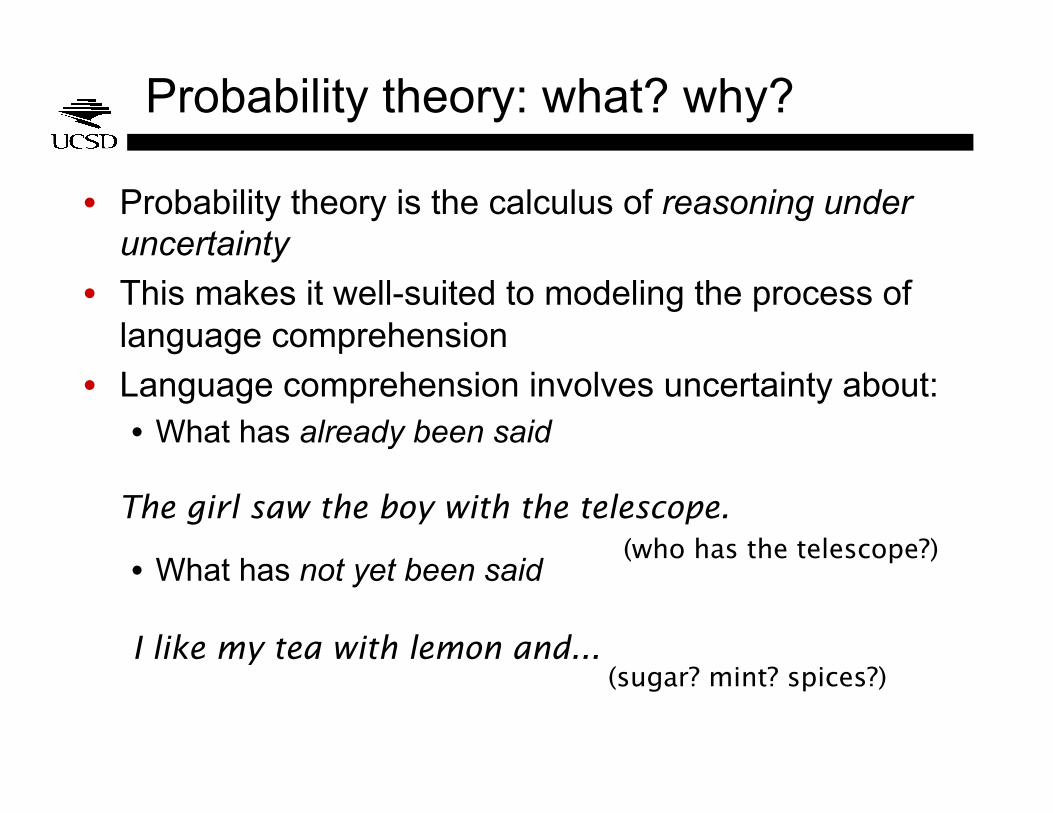
Probability theory: what? why?

•  Probability theory is the calculus of reasoning under uncertainty

•  This makes it well-suited to modeling the process of language comprehension

•  Language comprehension involves uncertainty about: •  What has already been said

•  What has not yet been said

The girl saw the boy with the telescope.

I like my tea with lemon and...

(who has the telescope?)

(sugar? mint? spices?)

Crash course in probability theory

•  Event space Ω

•  A function P from subsets of Ω to real numbers such that: •  Non-negativity:

•  Properness:

•  Disjoint union:

•  An improper function P for which is called deficient

Probability: an example

•  Rolling a die has event space Ω={1,2,3,4,5,6}

•  If it is a fair die, we require of the function P:

•  Disjoint union means that this requirement completely specifies the probability distribution P

•  For example, the event that a roll of the die comes out even is E={2,4,6}. For a fair die, its probability is

•  Using disjoint union to calculate event probabilities is known as the counting method

Joint and conditional probability

•  P(X,Y) is called a joint probability •  e.g., probability of a pair of dice coming out <4,6>

•  Two events are independent if the probability of the joint event is the product of the individual event probabilities:

•  P(Y|X) is called a conditional probability •  By definition,

•  This gives rise to Bayes’ Theorem:

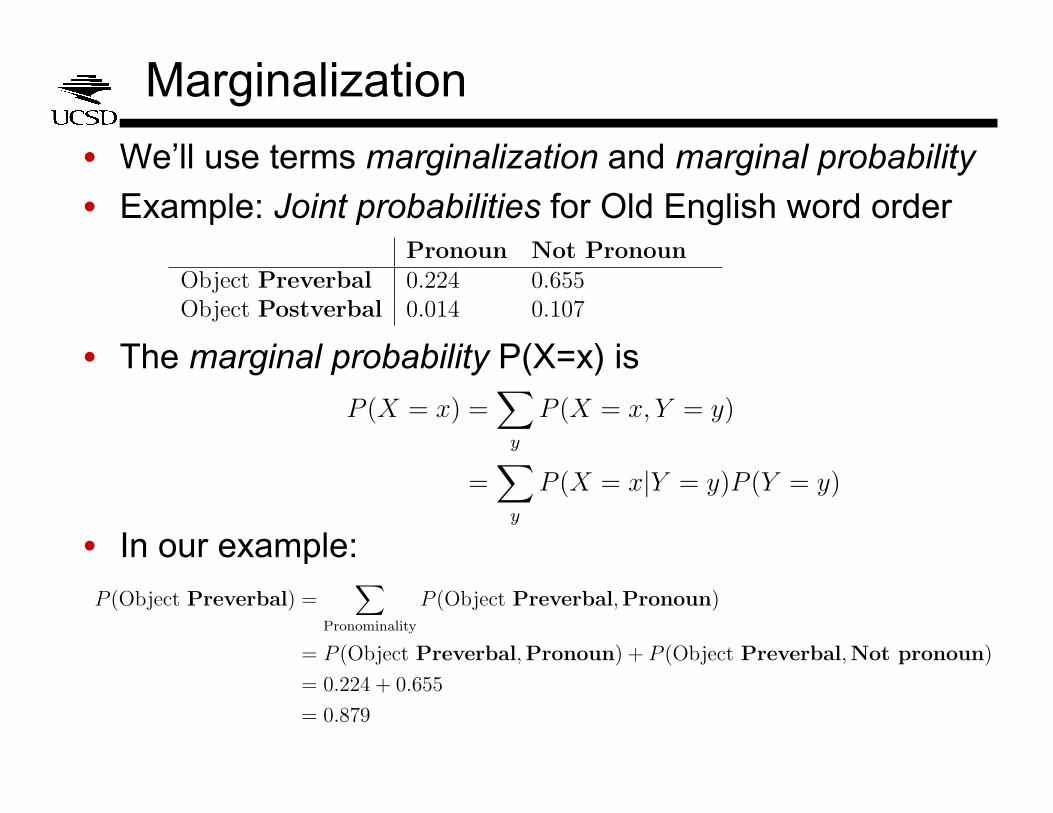
Marginalization

•  We’ll use terms marginalization and marginal probability

•  Example: Joint probabilities for Old English word order

•  The marginal probability P(X=x) is

•  In our example:

Pronoun Not Pronoun

Object Preverbal 0.224 0.655Object Postverbal 0.014 0.107

P (X = x) =!

y

P (X = x, Y = y)

=!

y

P (X = x|Y = y)P (Y = y)

P (Object Preverbal) =!

Pronominality

P (Object Preverbal,Pronoun)

= P (Object Preverbal,Pronoun) + P (Object Preverbal,Not pronoun)

= 0.224 + 0.655

= 0.879

Bayesian inference

•  We already saw Bayes’ rule as a consequence of the laws of conditional probability

•  Its importance is its use for inference and learning

•  The posterior distribution summarizes all the information relevant to decision-making about X on the basis of Y

P (X|Y ) =P (Y |X)P (X)

P (Y )

Observations (“data”)

Hidden structure

Prior probability of hidden structure

Likelihood of data given a particular hidden structure

(marginal likelihood of data)

Posterior distribution

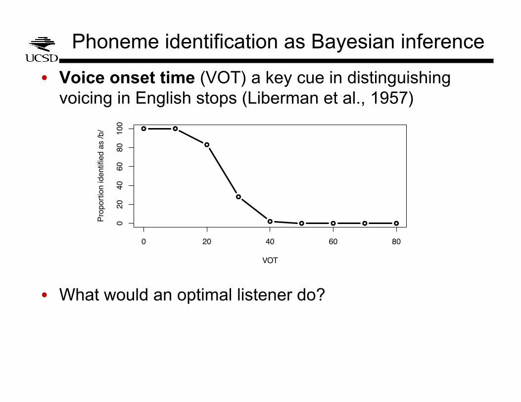
Phoneme identification as Bayesian inference

•  Voice onset time (VOT) a key cue in distinguishing voicing in English stops (Liberman et al., 1957)

•  What would an optimal listener do?

! !

!

!

! ! ! ! !

0 20 40 60 80

020

4060

8010

0

VOT

Prop

ortio

n id

entif

ied

as /b

/

−20 0 20 40 60 80

0.00

0.02

0.04

VOT

Prob

abilit

y de

nsity

[b] [p]


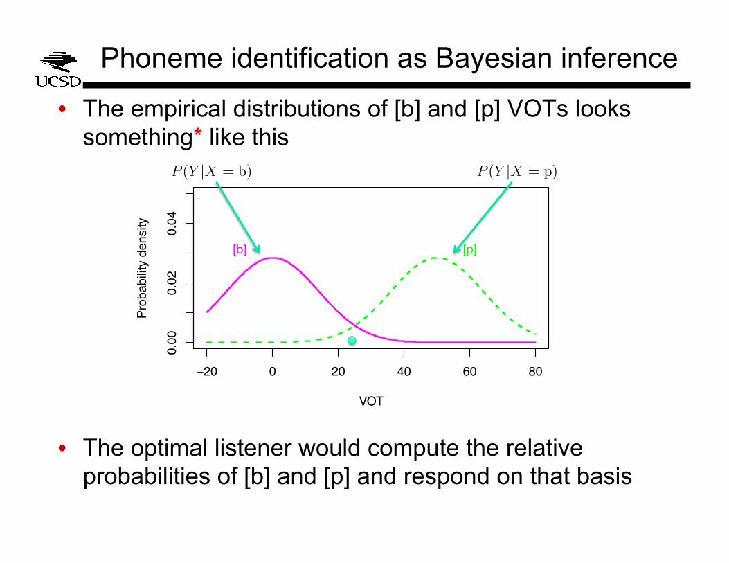
•  The empirical distributions of [b] and [p] VOTs looks something* like this

•  The optimal listener would compute the relative probabilities of [b] and [p] and respond on that basis

P (Y |X = b) P (Y |X = p)


•  To complete Bayesian inference for an input Y, we need to specify the likelihood functions

•  For likelihood, we’ll use the normal distribution:

•  And we’ll set the priors equal: P(X=b)=P(X=p)=0.5

P (X = b|Y ) =P (Y |X = b)P (X = b)

P (Y )

Likelihood Prior

Marginal likelihood

P (Y = y|X = x) =1

!

2!"2x

e!

(y!µx)2

2!2x

mean

variance

−20 0 20 40 60 80

0.00

0.02

0.04

VOT

Prob

abilit

y de

nsity

[b] [p]

−20 0 20 40 60 80

0.00

0.02

0.04

VOT

Prob

abilit

y de

nsity

[b] [p]

−20 0 20 40 60 80

0.0

0.2

0.4

0.6

0.8

1.0

VOT

Post

erio

r pro

babi

lity o

f /b/


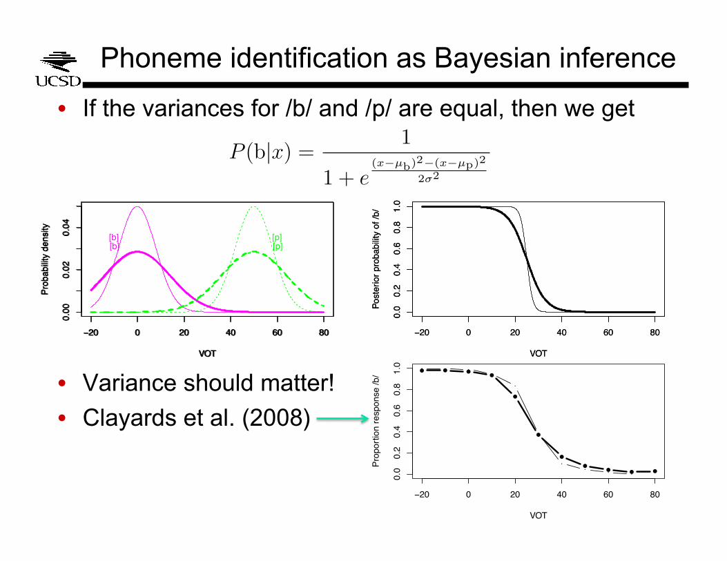
•  If the variances for /b/ and /p/ are equal, then we get

•  Variance should matter!

•  Clayards et al. (2008)

P (b|x) =1

1 + e(x!µb)2!(x!µp)2

2!2

−20 0 20 40 60 80

0.0

0.2

0.4

0.6

0.8

1.0

VOT

Post

erio

r pro

babi

lity o

f /b/

−20 0 20 40 60 80

0.0

0.2

0.4

0.6

0.8

1.0

VOT

Prop

ortio

n re

spon

se /b

/ ! ! !

!

!

!

!

!

!! !

−20 0 20 40 60 80

0.00

0.02

0.04

VOT

Prob

abilit

y de

nsity

[b] [p]

Estimating probabilistic models

•  With a fair die, we can calculate event probabilities using the counting method

•  But usually, we can’t deduce the probabilities of the subevents involved

•  Instead, we have to estimate them (=statistics!)

•  Usually, this involves assuming a probabilistic model with some free parameters,* and choosing the values of the free parameters to match empirically obtained data

*(these are parametric estimation methods)

Maximum likelihood

•  Simpler example: a coin flip •  fair? unfair?

•  Take a dataset of 20 coin flips, 12 heads and 8 tails

•  Estimate the probability p that the next result is heads

•  Method of maximum likelihood: choose parameter values (i.e., p) that maximize the likelihood* of the data

•  Here, maximum-likelihood estimate (MLE) is the relative-frequency estimate (RFE)

*likelihood: the data’s probability, viewed as a function of your free parameters

Issues in model estimation

•  Maximum-likelihood estimation has several problems: •  Can’t incorporate a belief that coin is “likely” to be fair

•  MLEs can be biased •  Try to estimate the number of words in a language from a

finite sample

•  MLEs will always underestimate the number of words

•  There are other estimation techniques with different strengths and weaknesses

•  In particular, there are Bayesian techniques that we’ll discuss later in the course (Lecture 7)

*unfortunately, we rarely have “lots” of data

Today




We’ll start with some puzzles

•  The women discussed the dogs on the beach. •  What does on the beach modify?

•  The women kept the dogs on the beach. •  What does on the beach modify?

•  The complex houses married children and their families.

•  The warehouse fires a dozen employees each year.

Ford et al., 1982→ dogs (90%); discussed (10%)

Ford et al., 1982→ kept (95%); dogs (5%)

Crash course in grammars and parsing

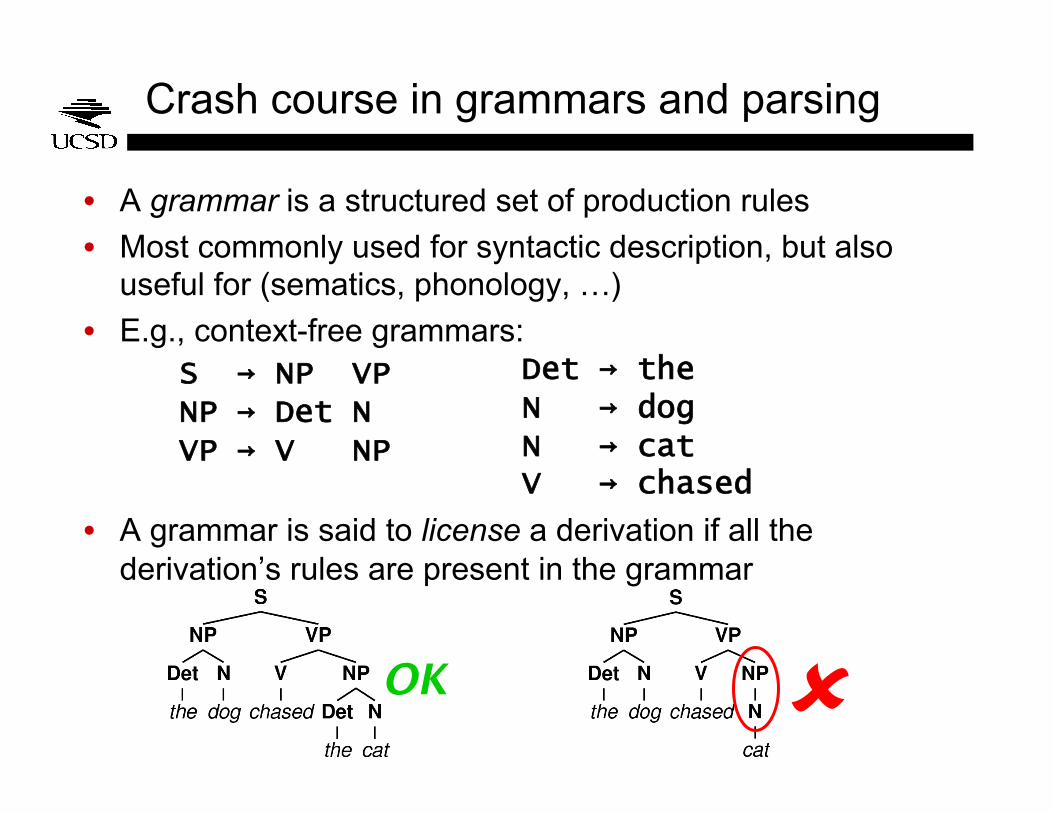
•  A grammar is a structured set of production rules

•  Most commonly used for syntactic description, but also useful for (sematics, phonology, …)

•  E.g., context-free grammars:

•  A grammar is said to license a derivation if all the derivation’s rules are present in the grammar

S → NP VP NP → Det N VP → V NP

Det → the N → dog N → cat V → chased

OK

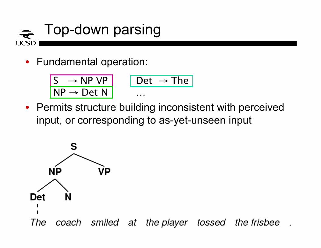
Top-down parsing

•  Fundamental operation:

•  Permits structure building inconsistent with perceived input, or corresponding to as-yet-unseen input

S → NP VP NP → Det N

Det → The …

Bottom-up parsing

•  Fundamental operation: check whether a sequence of categories matches a rule’s right-hand side

•  Permits structure building inconsistent with global context

VP → V NP PP → P NP

S → NP VP …

Ambiguity

•  There is usually more than one structural analysis for a (partial) sentence

•  Corresponds to choices (non-determinism) in parsing

•  VP can expand to V NP PP…

•  …or VP can expand to V NP and then NP can expand to NP PP

•  Ambiguity can be local (eventually resolved)… •  …with a puppy on his lap.

•  …or it can be global (unresolved): •  …with binoculars.

The girl saw the boy with…

Serial vs. Parallel processing

•  A serial processing model is one where, when faced with a choice, chooses one alternative and discards the rest

•  A parallel model is one where at least two alternatives are chosen and maintained •  A full parallel model is one where all alternatives are

maintained

•  A limited parallel model is one where some but not necessarily all alternatives are maintained

A joke about the man with an umbrella that I heard…

*ambiguity goes as the Catalan numbers (Church and Patel 1982)

Dynamic programming

•  There is an exponential number of parse trees for a given sentence (Church & Patil 1982)

•  So sentence comprehension can’t entail an exhaustive enumeration of possible structural representations

•  But parsing can be made tractable by dynamic programming

Dynamic programming (2)

•  Dynamic programming = storage of partial results •  There are two ways to make an NP out of…

•  …but the resulting NP can be stored just once in the parsing process

•  Result: parsing time polynomial (cubic for CFGs) in sentence length

•  Still problematic for modeling human sentence proc.

Hybrid bottom-up and top-down

•  Many methods used in practice are combinations of top-down and bottom-up regimens

•  Left-corner parsing: incremental bottom-up parsing with top-down filtering

•  Earley parsing: strictly incremental top-down parsing with top-down filtering and dynamic programming*

*solves problems of left-recursion that occur in top-down parsing

Probabilistic grammars

•  A (generative) probabilistic grammar is one that associates probabilities with rule productions.

•  e.g., a probabilistic context-free grammar (PCFG) has rule productions with probabilities like

•  Interpret P(NP→Det N) as P(Det N | NP)

•  Among other things, PCFGs can be used to achieve disambiguation among parse structures

a man arrived yesterday 0.3 S → S CC S 0.15 VP → VBD ADVP 0.7 S → NP VP 0.4 ADVP → RB 0.35 NP → DT NN ...

0.7

0.15 0.35

0.4 0.3 0.03 0.02

0.07

Total probability: 0.7*0.35*0.15*0.3*0.03*0.02*0.4*0.07= 1.85×10-7

Probabilistic grammars (2)

•  A derivation having zero probability corresponds to it being unlicensed in a non-probabilistic setting

•  But “canonical” or “frequent” structures can be distinguished from “marginal” or “rare” structures via the derivation rule probabilities

•  From a computational perspective, this allows probabilistic grammars to increase coverage (number + type of rules) while maintaining ambiguity management

Inference about sentence structure

•  With a probabilistic grammar, ambiguity resolution means inferring the probability distribution over structural analyses given input

•  Bayes Rule again

The girl saw the boy with…

Today




Pruning approaches

•  Jurafsky 1996: a probabilistic approach to lexical access and syntactic disambiguation

•  Main argument: sentence comprehension is probabilistic, construction-based, and parallel

•  Probabilistic parsing model explains •  human disambiguation preferences

•  garden-path sentences

•  The probabilistic parsing model has two components: •  constituent probabilities – a probabilistic CFG model

•  valence probabilities

Jurafsky 1996

•  Every word is immediately completely integrated into the parse of the sentence (i.e., full incrementality)

•  Alternative parses are ranked in a probabilistic model

•  Parsing is limited-parallel: when an alternative parse has unacceptably low probability, it is pruned

•  “Unacceptably low” is determined by beam search (described a few slides later)

Jurafsky 1996: valency model

•  Whereas the constituency model makes use of only phrasal, not lexical information, the valency model tracks lexical subcategorization, e.g.: P( <NP PP> | discuss ) = 0.24

P( <NP> | discuss ) = 0.76

(in today’s NLP, these are called monolexical probabilities)

•  In some cases, Jurafsky bins across categories:* P( <NP XP[+pred]> | keep) = 0.81

P( <NP> | keep ) = 0.19

where XP[+pred] can vary across AdjP, VP, PP, Particle…

*valence probs are RFEs from Connine et al. (1984) and Penn Treebank

Jurafsky 1996: syntactic model

•  The syntactic component of Jurafsky’s model is just probabilistic context-free grammars (PCFGs)

0.7

0.15 0.35

0.4 0.3 0.03 0.02

0.07

Total probability: 0.7*0.35*0.15*0.3*0.03*0.02*0.4*0.07= 1.85×10-7

Modeling offline preferences

•  Ford et al. 1982 found effect of lexical selection in PP attachment preferences (offline, forced-choice): •  The women discussed the dogs on the beach •  NP-attachment (the dogs that were on the beach) -- 90%

•  VP-attachment (discussed while on the beach) – 10%

•  The women kept the dogs on the beach •  NP-attachment – 5%

•  VP-attachment – 95%

•  Broadly confirmed in online attachment study by Taraban and McClelland 1988

Modeling offline preferences (2)

•  Jurafsky ranks parses as the product of constituent and valence probabilities:

Modeling offline preferences (3)

Result

•  Ranking with respect to parse probability matches offline preferences

•  Note that only monotonicity, not degree of preference is matched

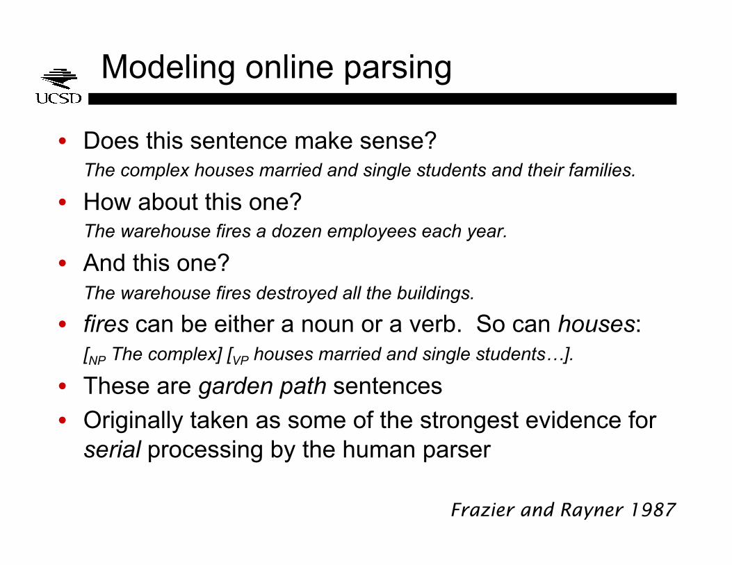
Modeling online parsing

•  Does this sentence make sense? The complex houses married and single students and their families.

•  How about this one? The warehouse fires a dozen employees each year.

•  And this one? The warehouse fires destroyed all the buildings.

•  fires can be either a noun or a verb. So can houses: [NP The complex] [VP houses married and single students…].

•  These are garden path sentences

•  Originally taken as some of the strongest evidence for serial processing by the human parser

Frazier and Rayner 1987

Limited parallel parsing

•  Full-serial: keep only one incremental interpretation

•  Full-parallel: keep all incremental interpretations

•  Limited parallel: keep some but not all interpretations

•  In a limited parallel model, garden-path effects can arise from the discarding of a needed interpretation

[S [NP The complex] [VP houses…] …]

[S [NP The complex houses …] …]

discarded

kept

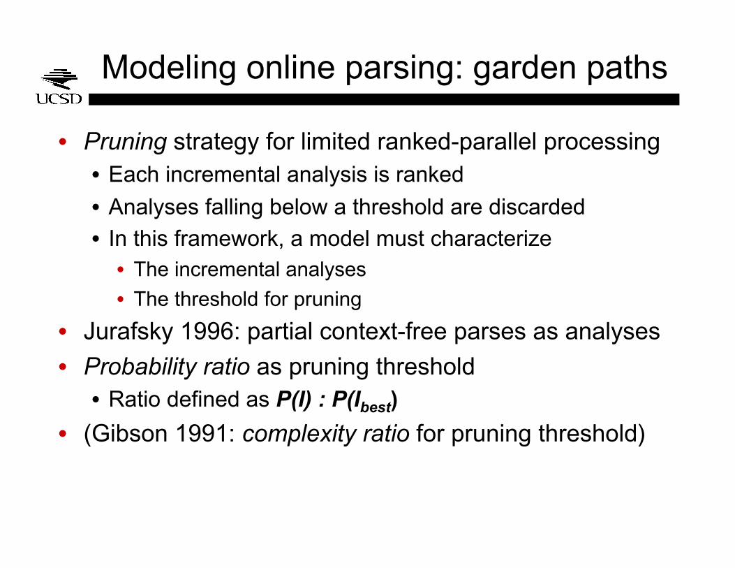
Modeling online parsing: garden paths

•  Pruning strategy for limited ranked-parallel processing •  Each incremental analysis is ranked

•  Analyses falling below a threshold are discarded

•  In this framework, a model must characterize •  The incremental analyses

•  The threshold for pruning

•  Jurafsky 1996: partial context-free parses as analyses

•  Probability ratio as pruning threshold •  Ratio defined as P(I) : P(Ibest)

•  (Gibson 1991: complexity ratio for pruning threshold)

Garden path models 1: N/V ambiguity

•  Each analysis is a partial PCFG tree

•  Tree prefix probability used for ranking of analysis

•  Partial rule probs marginalize over rule completions

these nodes are actually still undergoing expansion

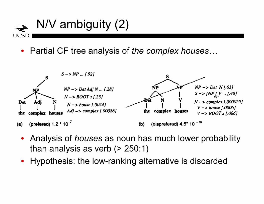
N/V ambiguity (2)

•  Partial CF tree analysis of the complex houses…

•  Analysis of houses as noun has much lower probability than analysis as verb (> 250:1)

•  Hypothesis: the low-ranking alternative is discarded

N/V ambiguity (3)

•  Note that top-down vs. bottom-up questions are immediately implicated, in theory

•  Jurafsky includes the cost of generating the initial NP under the S •  of course, it’s a small cost as P(S -> NP …) = 0.92

•  If parsing were bottom-up, that cost would not have been explicitly calculated yet

Garden path models 2

•  The most famous garden-paths: reduced relative clauses (RRCs) versus main clauses (MCs)

•  From the valence + simple-constituency perspective, MC and RRC analyses differ in two places:

The horse raced past the barn fell.

(that was)

p≈1 p=0.14

transitive valence: p=0.08

best intransitive: p=0.92

Garden path models 2, cont.

•  82 : 1 probability ratio means that lower-probability analysis is discarded

•  In contrast, some RRCs do not induce garden paths:

•  Here, the probability ratio turns out to be much closer (≈4 : 1) because found is preferentially transitive

•  Conclusion within pruning theory: beam threshold is between 4 : 1 and 82 : 1

•  (granularity issue: when exactly does probability cost of valence get paid???)

The bird found in the room died.

Notes on the probabilistic model

•  Jurafsky 1996 is a product-of-experts (PoE) model

•  Expert 1: the constituency model

•  Expert 2: the valence model

•  PoEs are flexible and easy to define, but hard to learn •  The Jurafsky 1996 model is actually deficient (loses

probability mass), due to relative frequency estimation

Notes on the probabilistic model (2)

•  Jurafsky 1996 predated most work on lexicalized parsers (Collins 1999, Charniak 1997)

•  In a generative lexicalized parser, valence and constituency are often combined through decomposition & Markov assumptions, e.g.,

•  The use of decomposition makes it easy to learn non-deficient models

sometimes approximated as

Jurafsky 1996 & pruning: main points

•  Syntactic comprehension is probabilistic

•  Offline preferences explained by syntactic + valence probabilities

•  Online garden-path results explained by same model, when beam search/pruning is assumed

General issues

•  What is the granularity of incremental analysis? •  In [NP the complex houses], complex could be an

adjective (=the houses are complex)

•  complex could also be a noun (=the houses of the complex)

•  Should these be distinguished, or combined?

•  When does valence probability cost get paid?

•  What is the criterion for abandoning an analysis?

•  Should the number of maintained analyses affect processing difficulty as well?

For Wednesday: surprisal

•  Read Hale, 2001, and the “surprisal” section of the Levy manuscript

•  The proposal is very simple:

•  Think about the following issues: •  How does surprisal differ from the Jurafsky 1996 model?

•  What is garden-path disambiguation under surprisal?

•  What kinds of probabilistic grammars are required for surprisal?

•  What kind of information belongs in “Context”?

Di!culty(wi) ! log1

P (wi|w1...i!1,Context)

lecture 1 lsa 2011-for-culearnidiom.ucsd.edu/.../lecture_1_lsa_2011-for-culearn.pdf ·...

Documents