lecture 1: matrix decompositions (chapter 4 of textbook a)

Lecture 1: Matrix Decompositions(Chapter 4 of Textbook A)

Jinwoo Shin

AI503: Mathematics for AI

This lecture slide is based uponhttps://yung-web.github.io/home/courses/mathml.html

(made by Prof. Yung Yi, KAIST EE)

https://yung-web.github.io/home/courses/mathml.html

Roadmap

(1) Determinant and Trace

(2) Eigenvalues and Eigenvectors

(3) Cholesky Decomposition

(4) Eigendecomposition and Diagonalization

(5) Singular Value Decomposition

(6) Matrix Approximation

(7) Matrix Phylogeny

Summary

• How to summarize matrices: determinants and eigenvalues

• How matrices can be decomposed: Cholesky decomposition, diagonalization,singular value decomposition

• How these decompositions can be used for matrix approximation

Roadmap








L4(1)

Determinant: Motivation (1)

• For A =

(a11 a12

a21 a22

), A−1 = 1

a11a22−a12a21

(a22 −a12

−a21 a11

).

• A is invertible iff a11a22 − a12a21 6= 0

• Let’s define det(A) = a11a22 − a12a21.

• Notation: det(A) or |whole matrix|

• What about 3× 3 matrix? By doing some algebra (e.g., Gaussian elimination),∣∣∣∣∣∣a11 a12 a13

a21 a22 a23

a31 a32 a33

∣∣∣∣∣∣ = a11a22a33 + a21a32a13 + a31a12a23

− a31a22a13 − a11a32a23 − a21a12a33

L4(1)

Determinant: Motivation (2)• Try to find some pattern ...

a11a22a33 + a21a32a13 + a31a12a23

− a31a22a13 − a11a32a23 − a21a12a33 =

a11(−1)1+1 det(A1,1) + a12(−1)1+2 det(A1,2)

+ a13(−1)1+3 det(A1,3)

- Ak,j is the submatrix of A that we obtainwhen deleting row k and column j .

source: www.cliffsnotes.com

• This is called Laplace expansion.

• Now, we can generalize this and provide the formal definition of determinant.

L4(1)

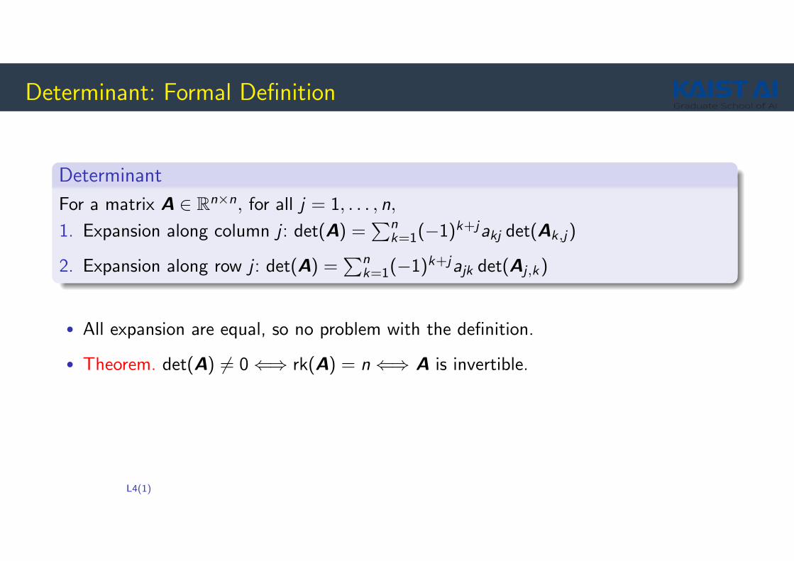
Determinant: Formal Definition

Determinant

For a matrix A ∈ Rn×n, for all j = 1, . . . , n,

1. Expansion along column j : det(A) =∑n

k=1(−1)k+jakj det(Ak,j)

2. Expansion along row j : det(A) =∑n

k=1(−1)k+jajk det(Aj ,k)

• All expansion are equal, so no problem with the definition.

• Theorem. det(A) 6= 0⇐⇒ rk(A) = n⇐⇒ A is invertible.

L4(1)

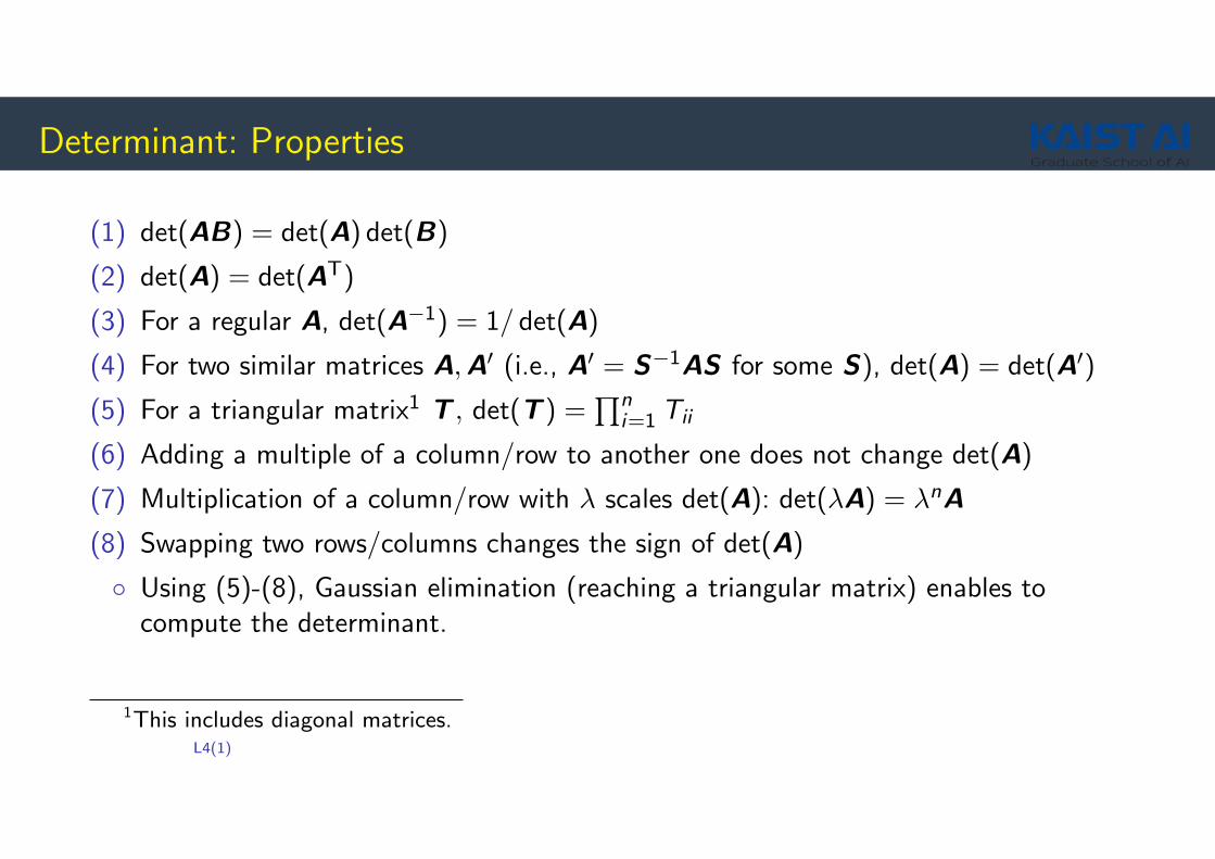
Determinant: Properties

(1) det(AB) = det(A) det(B)

(2) det(A) = det(AT)

(3) For a regular A, det(A−1) = 1/ det(A)

(4) For two similar matrices A,A′ (i.e., A′ = S−1AS for some S), det(A) = det(A′)(5) For a triangular matrix1 T , det(T ) =

∏ni=1 Tii

(6) Adding a multiple of a column/row to another one does not change det(A)

(7) Multiplication of a column/row with λ scales det(A): det(λA) = λnA(8) Swapping two rows/columns changes the sign of det(A)

◦ Using (5)-(8), Gaussian elimination (reaching a triangular matrix) enables tocompute the determinant.

1This includes diagonal matrices.L4(1)

Trace

• Definition. The trace of a square matrix A ∈ Rn×n is defined as

tr(A) :=n∑

i=1

aii

• tr(A + B) = tr(A) + tr(B)

• tr(αA) = α tr(A)

• tr(In) = n

L4(1)

Invariant under Cyclic Permutations

• tr(AB) = tr(BA) for A ∈ Rn×k and B ∈ Rk×n

• tr(AKL) = tr(KLA), for A ∈ Ra×k , K ∈ Rk×l , L ∈ Rl×a

• tr(xyT) = tr(yTx) = yTx ∈ R

• A linear mapping Φ : V 7→ V , represented by a matrix A and another matrix B.◦ A and B use different bases, where B = S−1AS

tr(B) = tr(S−1AS) = tr(ASS−1) = tr(A)

◦ Message. While matrix representations of linear mappings are basis dependent, but theirtraces are not.

L4(1)

Background: Characteristic Polynomial

• Definition. For λ ∈ R and a matrix A ∈ Rn×n, the characteristic polynomial of A isdefined as:

pA(λ) := det(A− λI )

= c0 + c1λ+ c2λ2 + · · ·+ cn−1λ

n−1 + (−1)nλn,

where c0 = det(A) and cn−1 = (−1)n−1 tr(A).

• Example. For A =

(4 21 3

),

pA(λ) =

∣∣∣∣4− λ 21 3− λ

∣∣∣∣ = (4− λ)(3− λ)− 2 · 1

L4(1)

Roadmap








L4(2)

Eigenvalue and Eigenvector

• Definition. Consider a square matrix A ∈ Rn×n. Then, λ ∈ R is an eigenvalue of Aand x ∈ Rn \ {0} is the corresponding eigenvector of A if

Ax = λx

• Equivalent statements◦ λ is an eigenvalue.

◦ (A− λIn)x = 0 can be solved non-trivially, i.e., x 6= 0.

◦ rk(A− λIn) < n.

◦ det(A− λIn) = 0 ⇐⇒ The characteristic polynomial pA(λ) = 0.

L4(2)

Example

• For A = ( 4 21 3 ), pA(λ) =

∣∣∣∣4− λ 21 3− λ

∣∣∣∣ = (4− λ)(3− λ)− 2 · 1 = λ2 − 7λ+ 10

• Eigenvalues λ = 2 or λ = 5.

• Eigenvector E5 for λ = 5(4− λ 2

1 3− λ

)x = 0 =⇒

(−1 21 −2

)(x1

x2

)= 0 =⇒ E5 = span[

(21

)]

• Eigenvector E2 for λ = 2. Similarly, we get E2 = span[

(1−1

)]

• Message. Eigenvectors are not unique.

L4(2)

Properties (1)

• If x is an eigenvector of A, so are all vectors that are collinear2.

• Eλ: the set of all eigenvectors for eigenvalue λ, spanning a subspace of Rn. We callthis eigensapce of A for λ.

• Eλ is the solution space of (A− λI )x = 0, thus Eλ = ker(A− λI )

• Geometric interpretation◦ The eigenvector corresponding to a nonzero eigenvalue points in a direction stretched by

the linear mapping.

◦ The eigenvalue is the factor of stretching.

• Identity matrix I : one eigvenvalue λ = 1 and all vectors x 6= 0 are eigenvectors.

2Two vectors are collinear if they point in the same or the opposite direction.L4(2)

Properties (2)

• A and AT share the eigenvalues, but not necessarily eigenvectors.

• For two similar matrices A,A′ (i.e., A′ = S−1AS for some S), they possess thesame eigenvalues.◦ Meaning: A linear mapping Φ has eigenvalues that are independent of the choice of

basis of its transformation matrix.

◦ Symmetric, positive definite matrices always have positive, real eigenvalues.

determinant, trace, eigenvalues: all invariant under basis change

L4(2)

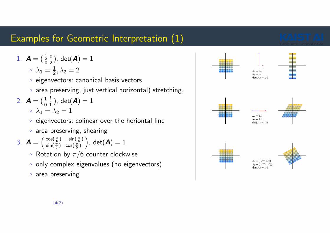
Examples for Geometric Interpretation (1)

1. A = (12 00 2

), det(A) = 1

◦ λ1 = 12 , λ2 = 2

◦ eigenvectors: canonical basis vectors

◦ area preserving, just vertical horizontal) stretching.

2. A = ( 1 12

0 1), det(A) = 1

◦ λ1 = λ2 = 1

◦ eigenvectors: colinear over the horiontal line

◦ area preserving, shearing

3. A =(

cos( π6 ) − sin( π

6 )

sin( π6 ) cos( π

6 )

), det(A) = 1

◦ Rotation by π/6 counter-clockwise

◦ only complex eigenvalues (no eigenvectors)

◦ area preserving

L4(2)

Examples for Geometric Interpretation (2)

4. A = ( 1 −1−1 1 ), det(A) = 0

◦ λ1 = 0, λ2 = 2

◦ Mapping that collapses a 2D onto 1D

◦ area collapses

5. A = (1 1

212 1

), det(A) = 3/4

◦ λ1 = 0.5, λ2 = 1.5

◦ area scales by 75%, shearing and stretching

L4(2)

Properties (3)

• For A ∈ Rn×n, n distinct eigenvalues =⇒ eigenvectors are linearly independent,which form a basis of Rn.◦ Converse is not true.

◦ Example of n linearly independent eigenvectors for less than n eigenvalues???

• Determinant. For (possibly repeated) eigenvalues λi of A ∈ Rn×n,

det(A) =∏n

i=1 λi

• Trace. For (possibly repeated) eigenvalues λi of A ∈ Rn×n,

tr(A) =∑n

i=1 λi

• Message. det(A) is the area scaling and tr(A) is the circumference scaling

L4(2)

Roadmap








L4(3)

LU Decomposition

Source: http://mathonline.wikidot.com/

• The Gaussian elimination is the processing of reaching an upper triangular matrix

• Gaussian elimination: multiplying the matrices corresponding to two elementaryoperations ((i) row multiplication by a and (ii) adding two rows downward)

• The above elementary operations are the low triangular matrices (LTM), and theirinverses and their product are all LTMs.

• (EkEk−1 · E1)A = U =⇒ A = (E1−1 · · ·Ek−1

−1Ek−1)︸︷︷︸

L

U

L4(3)

http://mathonline.wikidot.com/

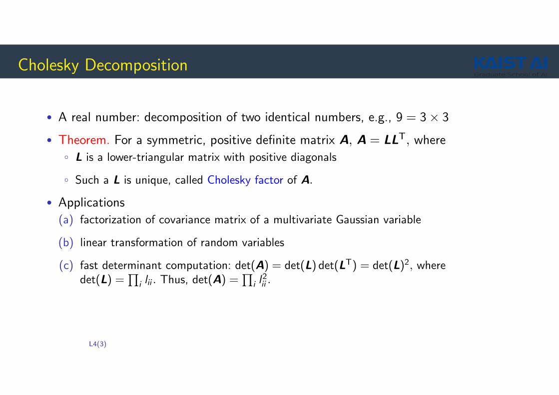
Cholesky Decomposition

• A real number: decomposition of two identical numbers, e.g., 9 = 3× 3

• Theorem. For a symmetric, positive definite matrix A, A = LLT, where◦ L is a lower-triangular matrix with positive diagonals

◦ Such a L is unique, called Cholesky factor of A.

• Applications

(a) factorization of covariance matrix of a multivariate Gaussian variable

(b) linear transformation of random variables

(c) fast determinant computation: det(A) = det(L) det(LT) = det(L)2, wheredet(L) =

∏i lii . Thus, det(A) =

∏i l

2ii .

L4(3)

Roadmap








L4(4)

Diagonal Matrix and Diagonalization

• Diagonal matrix. zero on all off-diagonal elements, D =

d1 · · · 0...

...0 · · · dn

Dk =

dk1 · · · 0...

...0 · · · dk

n

, D−1 =

1/d1 · · · 0...

...0 · · · 1/dn

, det(D) = d1d2 · · · dn

• Definition. A ∈ Rn×n is diagonalizable if it is similar to a diagonal matrix D, i.e., ∃an invertible P ∈ Rn×n, such that D = P−1AP.

• Definition. A ∈ Rn×n is orthogonally diagonalizable if it is similar to a diagonalmatrix D, i.e., ∃ an orthogonal P ∈ Rn×n, such that D = P−1AP = PTAP.

L4(4)

Power of Diagonalization

• Ak = PDkP−1

• det(A) = det(P) det(D) det(P−1) = det(D) =∏

i dii

• Many other things ...

• Question. Under what condition is A diagonalizable (or orthogonally diagonalizable)and how can we find P (thus D)?

L4(4)

Diagonalizablity, Algebraic/Geometric Multiplicity

• Definition. For a matrix A ∈ Rn×n with an eigenvalue λi ,◦ the algebraic multiplicity αi of λi is the number of times the root appears in the

characteristic polynomial.

◦ the geometric multiplicity ζi of λi is the number of linearly independent eigenvectorsassociated with λi (i.e., the dimension of the eigenspace spanned by the eigenvectors ofλi )

• Example. The matrix A =

(2 10 2

)has two repeated eigenvalues λ1 = λ2 = 2, thus

α1 = 2. However, it has only one distinct unit eigenvector x =

(10

), thus ζ1 = 1.

• Theorem. A ∈ Rn×n is diagonalizable ⇐⇒∑

i αi =∑

i ζi = n.

L4(4)

Orthogonally Diagonaliable and Symmetric Matrix

Theorem. A ∈ Rn×n is orthogonally diagonalizable ⇐⇒ A is symmetric.

• Question. . How to find P (thus D)?

• Spectral Theorem. If A ∈ Rn×n is symmetric,

(a) the eigenvalues are all real

(b) the eigenvectors to different eigenvalues are perpendicular.

(c) there exists an orthogonal eigenbasis

• For (c), from each set of eigenvectors, say {x1, . . . , xk} associated with a particulareigenvalue, say λj , we can construct another set of eigenvectors {x ′1, . . . , x ′k} thatare orthonormal, using the Gram-Schmidt process.

• Then, all eigenvectors can form an orthornormal basis.

L4(4)

Example

• Example. A =(

3 2 22 3 22 2 3

). pA(λ) = −(λ− 1)2(λ− 7), thus λ1 = 1, λ2 = 7

E1 = span[(−1

10

),(−1

01

)], E7 = span[

(111

)]

◦ (111)T is perpendicular to (−110)T and (−101)T

◦(−1

10

)and

(−1/2−1/2

1

)(for λ = 1) and

(111

)(for λ = 7) are the orthogonal basis in R3.

◦ After normalization, we can make the orthonormal basis.

L4(4)

Eigendecomposition

• Theorem. The following is equivalent.

(a) A square matrix A ∈ Rn×n can be factorized into A = PDP−1, where P ∈ Rn×n andD is the diagonal matrix whose diagonal entries are eigenvalues of A.

(b) The eigenvectors of A form a basis of Rn (i.e., The n eigenvectors of A are linearlyindependent)

• The above implies the columns of P are the n eigenvectors of A (becauseAP = PD)

• P is an orthogonal matrix, so PT = P−1

• A is symmetric, then (b) holds (Spectral Theorem).

L4(4)

Example of Orthogonal Diagonalization (1)

• Eigendecomposition for A =

(2 11 2

)• Eigenvalues: λ1 = 1, λ2 = 3

• (normalized) eigenvectors: p1 = 1√2

(1−1

), p2 = 1√

2

(11

).

• p1 and p2 linearly independent, so A is diagonalizable.

• P =(p1 p2

)= 1√

2

(1 1−1 1

)• D = P−1AP =

(1 00 3

). Finally, we get A = PDP−1

L4(4)

Example of Orthogonal Diagonalization (2)

• A =

1 2 22 1 22 2 1

• Eigenvalues: λ1 = −1, λ2 = 5

(α1 = 2, α2 = 1)

• E−1 = span[

−110

,

−101

]Gram-Schmidt−−−−−−−−→

span[ 1√2

−110

, 1√6

−112

]

• E5 = span[ 1√3

111

]

• P =

−1/√

2 −1/√

6 1/√

3

1/√

2 −1/√

6 1/√

3

0 2/√

6 1/√

3

• D = PTAP =

−1 0 00 −1 00 0 5

L4(4)

Eigendecomposition: Geometric Interpretation

Question. Can we generalize this beautiful result to a general matrix A ∈ Rm×n?

L4(4)

Roadmap








L4(5)

Storyline

• Eigendecomposition (also called EVD: EigenValue Decomposition): (Orthogoanl)Diagonalization for symmetric matrices A ∈ Rn×n.

• Extensions: Singular Value Decomposition (SVD)

1. First extension: diagonalization for non-symmetric, but still square matrices A ∈ Rn×n

2. Second extension: diagonalization for non-symmeric, and non-square matrices A ∈ Rm×n

• Background. For A ∈ Rm×n, a matrix S := ATA ∈ Rn×n is always symmetric,positive semidefinite.

◦ Symmetric, because ST = (ATA)T

= ATA = S .

◦ Positive semidefinite, because xTSx = xTATAx = (Ax)T(Ax) ≥ 0.

◦ If rk(A) = n, then symmetric and positive definite.

L4(5)

Singular Value Decomposition

• Theorem. A ∈ Rm×n with rank r ∈ [0,min(m, n)]. The SVD of A is adecomposition of the form

A = UΣV T,

with an orthogonal matrix U =(u1 · · · um

)∈ Rm×m and an orthogonal matrix

V =(v1 · · · vn

)∈ Rn×n. Moreoever, Σ s an m × n matrix with Σii = σi ≥ 0 and

Σij = 0, i 6= j , which is uniquely determined for A.

• Note◦ The diagonal entries σi , i = 1, . . . , r are called singular values.

◦ ui and vj are called left and right singular vectors, respectively.

L4(5)

SVD: How It Works (for A ∈ Rn×n)

• A ∈ Rn×n with rank r ≤ n. Then, ATA issymmetric.

• Orthogonal diagonalization of ATA:

ATA = VDV T.

• D =

(λ1

. . .λn

)and an orthogonal matrix

V =(v1 · · · vn

), where

λ1 ≥ · · · ≥ λr ≥ λr+1 = · · ·λn = 0 are theeigenvalues of ATA and {vi} areorthonormal.

• All λi are positive

∀x ∈ Rn, ‖Ax‖2 = AxTAx = xTATAx = λi ‖x‖2

• rk(A) =rk(ATA) = rk(D) =r

• Choose U ′ =(u1 · · ·ur

), where

ui =Avi√λi, 1 ≤ i ≤ r .

• We can construct {ui}, i = r + 1, · · · , n, sothat U =

(u1 · · ·un

)is an orthonormal

basis of Rn.

• Define Σ =

(√λ1

. . . √λn

)• Then, we can check that UΣ = AV .• Similar arguments for a general A ∈ Rm×n

(see pp. 104)

L4(5)

Example

• A =

(1 0 1−2 1 0

)

• ATA =

5 −2 1−2 1 01 0 1

= VDV T,

D =

6 0 00 1 00 0 0

,V =

5√30

−2√30

1√30

0 1√5

2√5

−1√6

−2√6

1√6

• rk(A) = 2 because we have two singular

values σ1 =√

6 and σ2 = 1

• Σ =

(√6 0 0

0 1 0

)

• u1 = Av1/σ1 =

(1√5−2√

5

)

• u2 = Av2/σ2 =

(2√5

1√5

)

• U =(u1 u2

)= 1√

5

(1 2−2 1

)• Then, we can see that A = UΣV T.

L4(5)

EVD (A = PDP−1) vs. SVD (A = UΣV T)

• SVD: always exists, EVD: square matrix and exists if we can find a basis ofeigenvectors (such as symmetric matrices)

• P in EVD is not necessarily orthogonal (only true for symmetric A), but U and Vare orthogonal (so representing rotations)

• Both EVD and SVD: (i) basis change in the domain, (ii) independent scaling ofeach new basis vector and mapping from domain to codomain, (iii) basis change inthe codomain. The difference: for SVD, different vector spaces of domain andcodomain.

• SVD and EVD are closely related through their projections◦ The left-singular (resp. right-singular) vectors of A are eigenvectors of AAT (resp. ATA)

◦ The singular values of A are the square roots of eigenvalues of AAT and ATA◦ When A is symmetric, EVD = SVD (from spectral theorem)

L4(5)

Different Forms of SVD

• When rk(A) = r , we can construct SVD as the following with only non-zerodiagonal entries in Σ:

A =

m×r︷︸︸︷U

r×r︷︸︸︷Σ

r×n︷︸︸︷V T

• We can even truncate the decomposed matrices, which can be an approximation ofA: for k < r

A ≈m×k︷︸︸︷U

k×k︷︸︸︷Σ

k×n︷︸︸︷V T

We will cover this in the next slides.

L4(5)

Matrix Approximation via SVD

• A =∑r

i=1 σi

Ai︷︸︸︷uiviT, where Ai is the outer product3 of ui and vi

• Rank k-approximation: A(k) =∑k

i=1 σiAi , k < r

3If u and v are both nonzero, then the outer product matrix uvvT always has matrix rank 1.Indeed, the columns of the outer product are all proportional to the first column.

L4(6)

How Close A(k) is to A?

• Definition. Spectral Norm of a Matrix. For A ∈ Rm×n, ‖A‖2 := maxx‖Ax‖2

‖x‖2◦ As a concept of length of A, it measures how long any vector x can at most become,

when multiplied by A

• Theorem. Eckart-Young. For A ∈ Rm×n of rank r and B ∈ Rm×n of rank k , for anyk ≤ r , we have:

A(k) = arg minrk(B)=k

‖A− B‖2 , and∥∥∥A− A(k)

∥∥∥2

= σk+1

◦ Quantifies how much error is introduced by the SVD-based approximation

◦ A(k) is optimal in the sense that such SVD-based approximation is the best one amongall rank-k approximations.

◦ In other words, it is a projection of the full-rank matrix A onto a lower-dimensionalspace of rank-at-most-k matrices.

L4(6)

Roadmap








L4(7)

Phylogenetic Tree of Matrices

L4(7)

Questions?

L4(7)

lecture 1: matrix decompositions (chapter 4 of textbook a)

Documents