1

Parallel computing, models and their performances

A high level exploration of the HPC

world

George Bosilca bosilca@eecs.utk.edu

University of Tennessee, Knoxville Innovative Computer Laboratory

Overview

•  Definition of parallel application •  Architectures taxonomy •  Laws managing the parallel domain •  Models in parallel computation •  Examples

2

Formal definition

Bernstein { I1 ∩ O2 = ∅ and I2 ∩ O1 = ∅ and O1 ∩ O2 = ∅ } General case: P1… Pn are parallel if and only if

each for each pair Pi, Pj we have Pi || Pj. 3 limit to the parallel applications:

1.  Data dependencies 2.  Flow dependencies 3.  Resources dependencies

P1 I1

O1 P2

I2

O2

Data dependencies

I1: A = B + C I2: E = D + A I3: A = F + G

I1

I2

I3

Dataflow dependency Anti-dependency

Output dependency How to avoid them? Which can be avoided ?

3

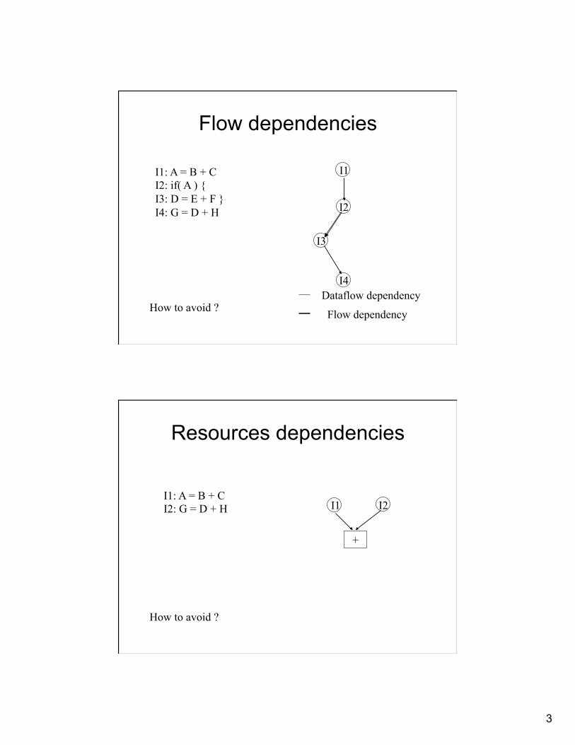
Flow dependencies

I1: A = B + C I2: if( A ) { I3: D = E + F } I4: G = D + H

I1

I2

I3

I4

Flow dependency

Dataflow dependency How to avoid ?

Resources dependencies

I1: A = B + C I2: G = D + H I1 I2

+

How to avoid ?

4

Flynn Taxonomy

1 Instruction flow

> 1 Instruction flow

1 data stream

SISD Von Neumann

MISD pipeline

> 1 data stream

SIMD MIMD

• Computers classified by instruction delivery mechanism and data stream • 4 characters code: 2 for instruction stream and 2 for data stream

Flynn Taxonomy: Analogy

•  SISD: lost people in the desert •  SIMD: rowing •  MISD: pipeline in the car construction

chain •  MIMD: airport facility, several desks

working at their own pace, synchronizing via a central database.

5

•  First law of parallel applications (1967) •  Limit the speedup for all parallel

applications

Amdahl Law

s

p

( )N

aaspeedup

Nps

psspeedup

−+=

+

+=

11

N = number of processors

Amdahl Law

Speedup is bound by 1/a.

6

Amdahl Law

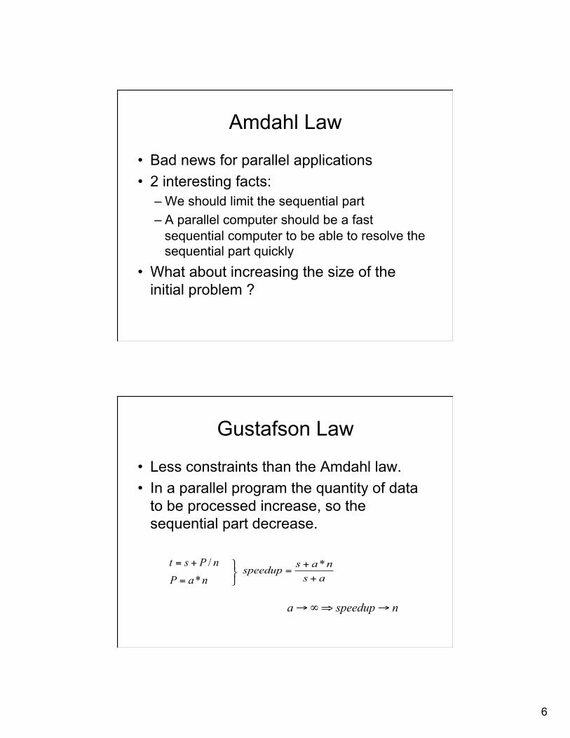
•  Bad news for parallel applications •  2 interesting facts:

– We should limit the sequential part – A parallel computer should be a fast

sequential computer to be able to resolve the sequential part quickly

•  What about increasing the size of the initial problem ?

Gustafson Law

•  Less constraints than the Amdahl law. •  In a parallel program the quantity of data

to be processed increase, so the sequential part decrease.

nPst /+=

naP *= asnasspeedup

+

+=

!"# *

nspeedupa →⇒∞→

7

Gustafson Law

•  The limit of Amdahl Law can be transgressed if the quantity of data to be processed increase.

snnspeedup )1( −+≤

Rule stating that if the size of most problems is scaled up sufficiently, then any required efficiency can be achieved on any number of processors.

Speedup

•  Superlinear speedup ? Sub-linear

Superlinear

Sometimes superlinear speedups can be observed! • Memory/cache effects • More processors typically also provide more memory/cache. • Total computation time decreases due to more page/cache hits.

• Search anomalies • Parallel search algorithms. • Decomposition of search range and/or multiple search strategies. • One task may be "lucky" to find result early.

8

Parallel execution models

•  Amdahl and Gustafson laws define the limits without taking in account the properties of the computer architecture.

•  They cannot be used to predict the real performance of any parallel application.

•  We should integrate in the same model the architecture of the computer and the architecture of the application.

What are models good for ?

•  Abstracting the computer properties – Making programming simple – Making programs portable ?

•  Reflecting essential properties – Functionality – Costs

•  What is the von-Neumann model for parallel architectures ?

9

Parallel Random Access Machine

•  One of the most studied •  World described as a collection of

synchronous processors which communicate with a global shared memory unit.

P1 P2 P3 P4

Shared memory

How to represent the architecture

•  2 resources have a major impact on the performances: – The couple (processor, memory) – The communication network.

•  The application should be described using those 2 resources.

Tapp = Tcomp + Tcomm

10

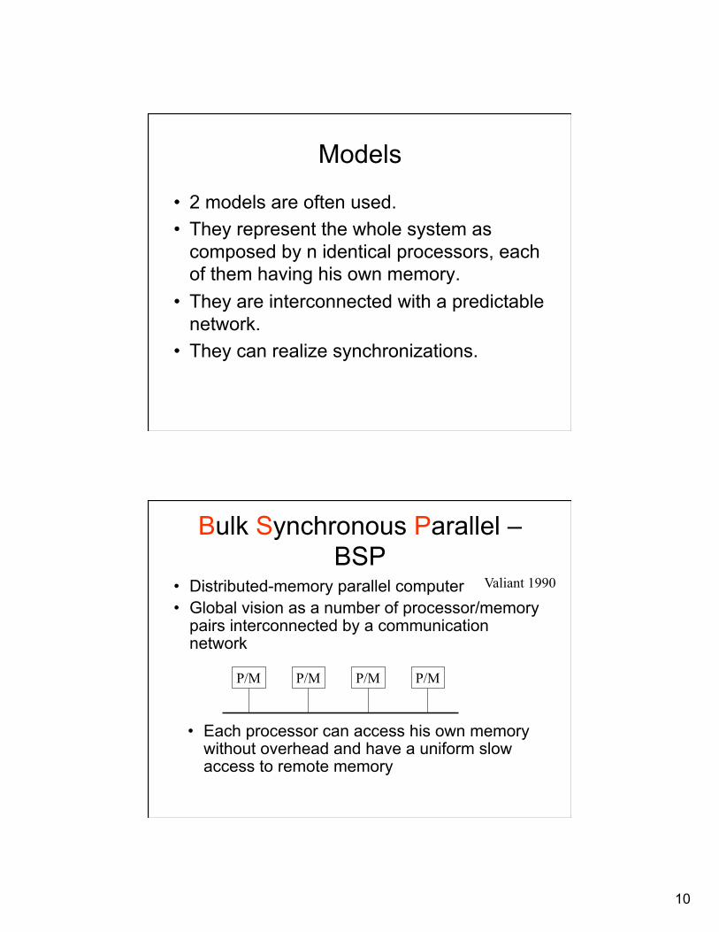
Models

•  2 models are often used. •  They represent the whole system as

composed by n identical processors, each of them having his own memory.

•  They are interconnected with a predictable network.

•  They can realize synchronizations.

Bulk Synchronous Parallel – BSP

•  Distributed-memory parallel computer •  Global vision as a number of processor/memory

pairs interconnected by a communication network

Valiant 1990

P/M P/M P/M P/M

•  Each processor can access his own memory without overhead and have a uniform slow access to remote memory

11

BSP

•  Applications composed by Supersteps separated by global synchronizations.

•  One superstep include: – A computation step – A communication step – A synchronization step

dependencies

Synchronization used to insure that all processors complete the computation + communication steps in the same amount of time.

BSP

Timeline

12

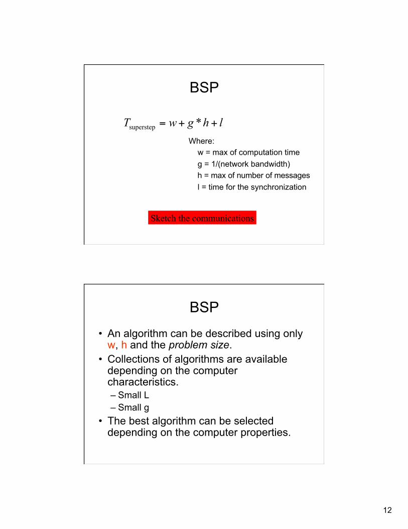
BSP

Where: w = max of computation time g = 1/(network bandwidth) h = max of number of messages l = time for the synchronization

lhgwT ++= *superstep

Sketch the communications

BSP

•  An algorithm can be described using only w, h and the problem size.

•  Collections of algorithms are available depending on the computer characteristics. – Small L – Small g

•  The best algorithm can be selected depending on the computer properties.

13

BSP - example

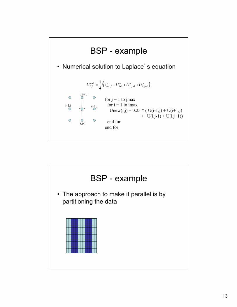
•  Numerical solution to Laplace’s equation

( )nji

nji

ni

nji

nji UUUUU 1,1,1,11

, 41

+−+−+ +++=

i,j+1

i,j-1

i+1,j i-1,j

for j = 1 to jmax for i = 1 to imax Unew(i,j) = 0.25 * ( U(i-1,j) + U(i+1,j) + U(i,j-1) + U(i,j+1)) end for end for

BSP - example

•  The approach to make it parallel is by partitioning the data

14

BSP - example

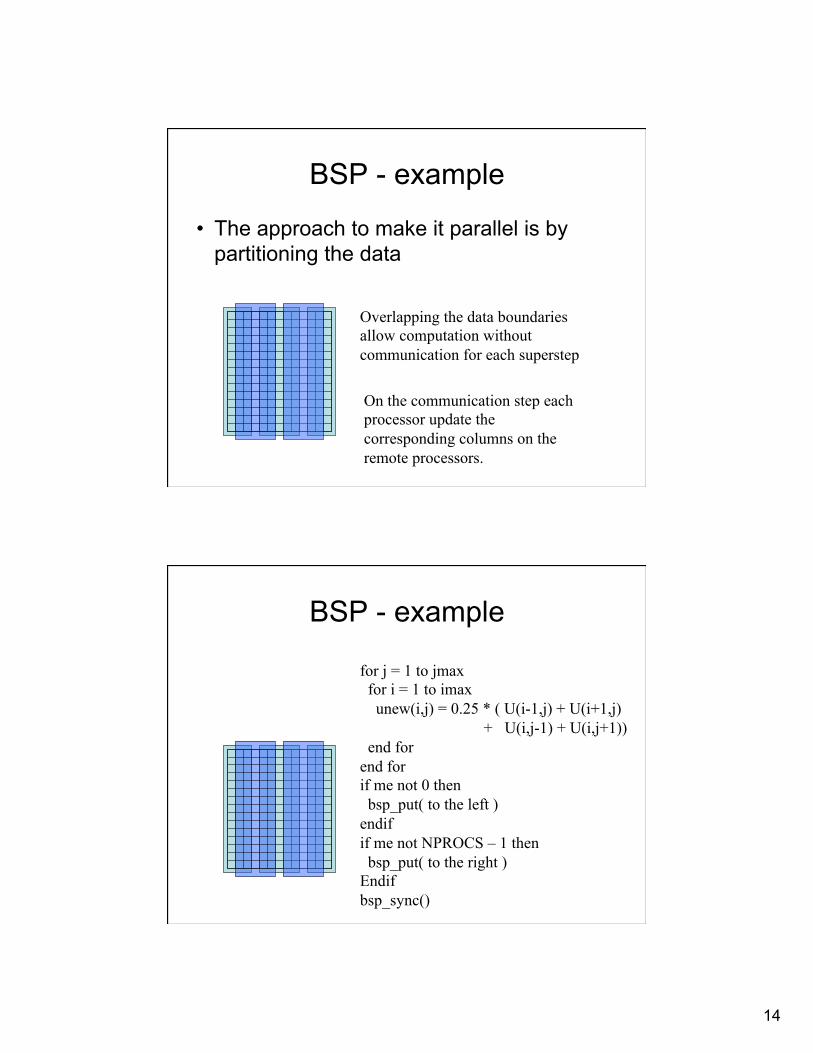
•  The approach to make it parallel is by partitioning the data

Overlapping the data boundaries allow computation without communication for each superstep

On the communication step each processor update the corresponding columns on the remote processors.

BSP - example

for j = 1 to jmax for i = 1 to imax unew(i,j) = 0.25 * ( U(i-1,j) + U(i+1,j) + U(i,j-1) + U(i,j+1)) end for end for if me not 0 then bsp_put( to the left ) endif if me not NPROCS – 1 then bsp_put( to the right ) Endif bsp_sync()

15

BSP - example

h = max number of messages = I values to the left + I values to the right = 2 * I (ignoring the inverse

communication!) w = 4 * I * I / p

lhgwT ++= *superstep

lIgpIT ++= **242

superstep

BSP - example

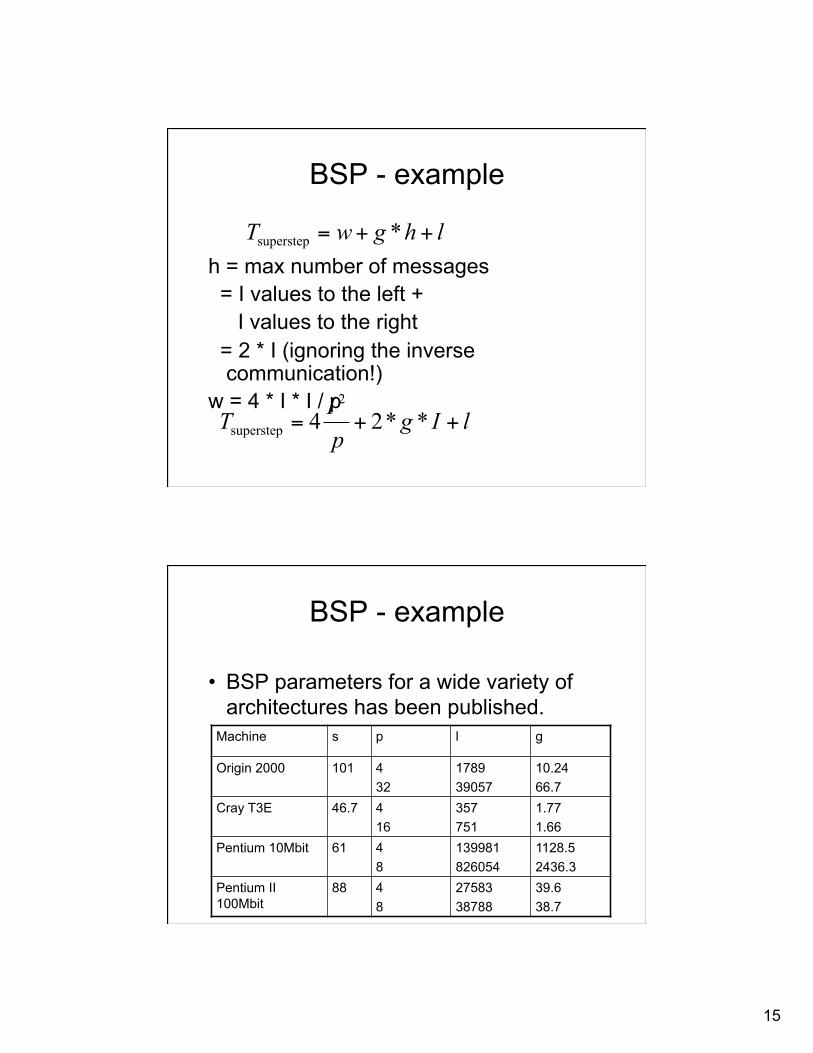
•  BSP parameters for a wide variety of architectures has been published.

Machine s p l g

Origin 2000 101 4 32

1789 39057

10.24 66.7

Cray T3E 46.7 4 16

357 751

1.77 1.66

Pentium 10Mbit 61 4 8

139981 826054

1128.5 2436.3

Pentium II 100Mbit

88 4 8

27583 38788

39.6 38.7

16

A more sophisticated model LogP

•  Tend to be more empirical and network-related.

P1 P2 P3 P4

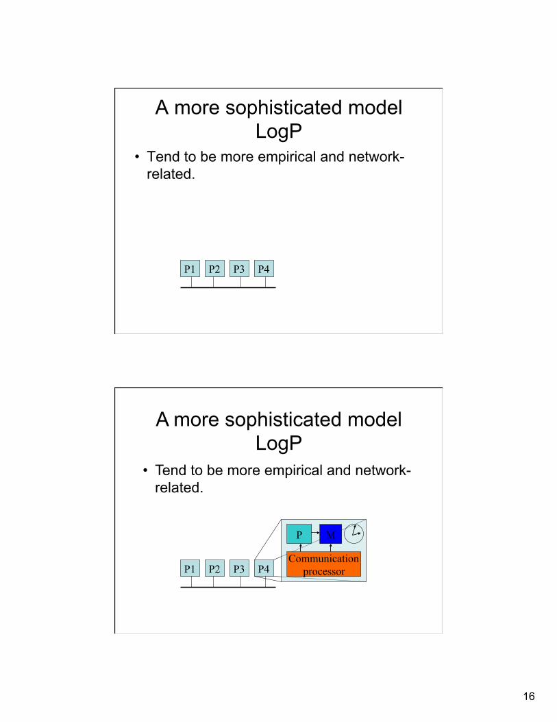
A more sophisticated model LogP

•  Tend to be more empirical and network-related.

P1 P2 P3 P4 Communication

processor

P M

17

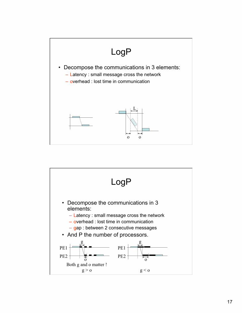
LogP

•  Decompose the communications in 3 elements: –  Latency : small message cross the network –  overhead : lost time in communication

o o

L

LogP

•  Decompose the communications in 3 elements: –  Latency : small message cross the network –  overhead : lost time in communication –  gap : between 2 consecutive messages

•  And P the number of processors. g

o

PE1

PE2

Both g and o matter ! g > o

g

o

PE1

PE2

g < o

18

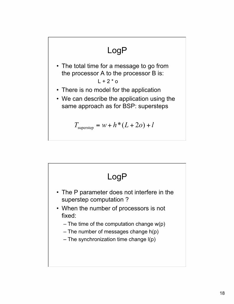
LogP

•  The total time for a message to go from the processor A to the processor B is:

L + 2 * o •  There is no model for the application •  We can describe the application using the

same approach as for BSP: supersteps

loLhwT +++= )2(*superstep

LogP

•  The P parameter does not interfere in the superstep computation ?

•  When the number of processors is not fixed: – The time of the computation change w(p) – The number of messages change h(p) – The synchronization time change l(p)

19

LogP

•  Allow/encourage the usage of general techniques of designing algorithms for distributed memory machines: exploiting locality, reducing communication complexity and overlapping communication and computation.

•  Balanced communication to avoid overloading the processors.

•  Interesting concept : idea of finite capacity of the network. Any attempt to transit more than a certain amount of data will stall the processor.

•  This model does not address on the issue of

message size, even the worst is the assumption of all messages are of ``small'' size.

•  Does not address the global capacity of the network.

LogP

!!

"##

$

gL

20

Design a LogP program

•  Execution time is the time of the slowest process

•  Implications for algorithms: – Balance computation – Balance communications Are only sub-goals !

•  Remember the capacity constraint !!

"##

$

gL

LogP Machines

21

Improving LogP •  First model to break the synchrony of parallel

execution •  LogGP : augments the LogP model with a linear

model for long messages •  LogGPC model extends the LogGP model to

include contention analysis using queuing model on the k-ary n-cubes network

•  LogPQ model augments the LogP model on the stalling issue of the network constraint by adding buffer queues in the communication lines.

The CCM model

•  Collective Computing Model transform the BSP superstep framework to support high-level programming models as MPI and PVM.

•  Remove the requirement of global synchronization between supersteps, but combines the message exchanges and synchronization properties into the execution of a collective communication.

•  Prediction quality usually high.