lecture 10,11 basics of fem

Dr. S.Meenatchi Sundaram, Department of Instrumentation & Control Engineering, MIT, Manipal

ICE 4010: MICRO ELECTRO MECHANICAL SYSTEMS (MEMS)

Lecture #10, 11

Finite Element Analysis

Dr. S. Meenatchi Sundaram

Email: [email protected]

1

Finite Element Methods

� Finite element method (FEM) is a numerical method to solve engineering problems with

complex geometries, materials and loads by converting a continuum into a discrete system.

� It has been applied to a number of physical problems, where the governing

differential equations are available.

� The method essentially consists of assuming the piecewise continuous function for the

solution and obtaining the parameters of the functions in a manner that reduces the error in

the solution.

� The finite element method involves modeling the structure using small interconnected

elements called finite elements.

� A displacement function is associated with each finite element.

� Every interconnected element is linked, directly or indirectly, to every other element

through common (or shared) interfaces, including nodes and/or boundary lines and/or

surfaces.

2S.Meenatchisundaram, Department of Instrumentation & Control Engineering, MIT, Manipal


� By using known stress/strain properties for the material making up the structure, one can

determine the behavior of a given node in terms of the properties of every other element in

the structure.

� The total set of equations describing the behavior of each node results in a series of

algebraic equations best expressed in matrix notation.

� There are two general direct approaches traditionally associated with the finite element

method as applied to structural mechanics problems.

� One approach, called the force, or flexibility method, uses internal forces as the unknowns

of the problem.

� To obtain the governing equations, first the equilibrium equations are used. Then necessary

additional equations are found by introducing compatibility equations.

� The result is a set of algebraic equations for determining the redundant or unknown forces.



� The second approach, called the displacement, or stiffness method, assumes the

displacements of the nodes as the unknowns of the problem.

� For instance, compatibility conditions requiring that elements connected at a common

node, along a common edge, or on a common surface before loading remain connected at

that node, edge, or surface after deformation takes place are initially satisfied.

� Then the governing equations are expressed in terms of nodal displacements using the

equations of equilibrium and an applicable law relating forces to displacements.

� These two direct approaches result in different unknowns (forces or displacements) in the

analysis and different matrices associated with their formulations (flexibilities or

stiffnesses).

� It has been shown that, for computational purposes, the displacement (or stiffness) method

is more desirable because its formulation is simpler for most structural analysis problems.



� Furthermore, a vast majority of general-purpose finite element programs have incorporated

the displacement formulation for solving structural problems.

� Another general method that can be used to develop the governing equations for both

structure and nonstructural problems is the variational method.

� The variational method includes a number of principles. One of these principles

extensively used is the theorem of minimum potential energy that applies to materials

behaving in a linear-elastic manner.


Formulation of Finite Element Methods

Step 1:Discretize and Select the Element Types:

� Discretization involves dividing the body into an equivalent system of finite elements with

associated nodes and choosing the most appropriate element type to model most closely

the actual physical behavior.

� The total number of elements used and their variation in size and type within a given body

are primarily matters of engineering judgment.

� The elements must be made small enough to give usable results and yet large enough to

reduce computational effort.

� Small elements (and possibly higher-order elements) are generally desirable where the

results are changing rapidly, such as where changes in geometry occur; large elements can

be used where results are relatively constant.

� The discretized body or mesh is often created with mesh-generation programs or

preprocessor programs available to the user.



(a) Simple two-noded tine element (typically used to represent a bar or beam element) and

the higher-order line element

(b) Simple two-dimensional elements with corner nodes (typically used to represent

plane stress/strain) and higher-order two-dimensional elements with intermediate

nodes along the sides



(c) Simple three-dimensional elements (typically used to represent three-dimensional stress

state) and higher-order three-dimensional elements with intermediate nodes along edges

(d) Simple axisymmetric triangular-and quadrilateral elements used for

axisymmetric problems



Step 2: Selection of Displacement Function:

� It involves choosing a displacement function within each element. The function is defined

within the element using the nodal values of the element.

� Linear, quadratic, and cubic polynomials are frequently used functions because they are

simple to work with in finite element formulation. However, trigonometric series can also

be used. For a two-dimensional element, the displacement function is a function of the

coordinates in its plane (the x-y plane).

� The functions are expressed in terms of the nodal unknowns (in the two-dimensional

problem, in terms of an x and a y component). The same general displacement function can

be used repeatedly for each element.

� Hence the finite element method is one in which a continuous quantity, such as the

displacement throughout the body, is approximated by a discrete model composed of a set

of piecewise-continuous functions defined within each finite domain or finite element.



Step 3: Define the Strain/Displacement and Stress/Strain Relationships:

� Strain/displacement and stress/strain, relationships are necessary for deriving the equations

for each finite element. In the case of one-dimensional deformation, say, in the x direction,

we have strain εx related to displacement u by

(1.1)

for small strains. In addition, the stresses must be related to the strains through the

stress/strain law-generally called the constitutive law. The ability to define the material

behavior accurately is most important in obtaining acceptable results. The simplest of

stress/strain laws, Hooke's law, which is often used in stress analysis, is given by

(1.2)

where = stress in the x direction and E = modulus of elasticity.



Step 4: Derive the Element Stiffness Matrix and Equations:

� Initially, the development of element stiffness matrices and element equations as based on

the concept of stiffness influence coefficients, which presupposes a background in

structural analysis. The alternative methods used are given below.

Direct Equilibrium Method:

According to this method, the stiffness matrix and element equations relating nodal forces

to nodal displacements are obtained using force equilibrium conditions for a basic element,

along with force/deformation relationships. This method is most easily adaptable to line or

one-dimensional elements, such as spring, bar, and beam elements.

To develop the stiffness matrix and equations for two- and three-dimensional elements, it is

much easier to apply a work or energy method. The principle of virtual work (using virtual

displacements), the principle of minimum potential energy, and Castigliano’s theorem are

methods frequently used for the purpose of derivation of element equations.



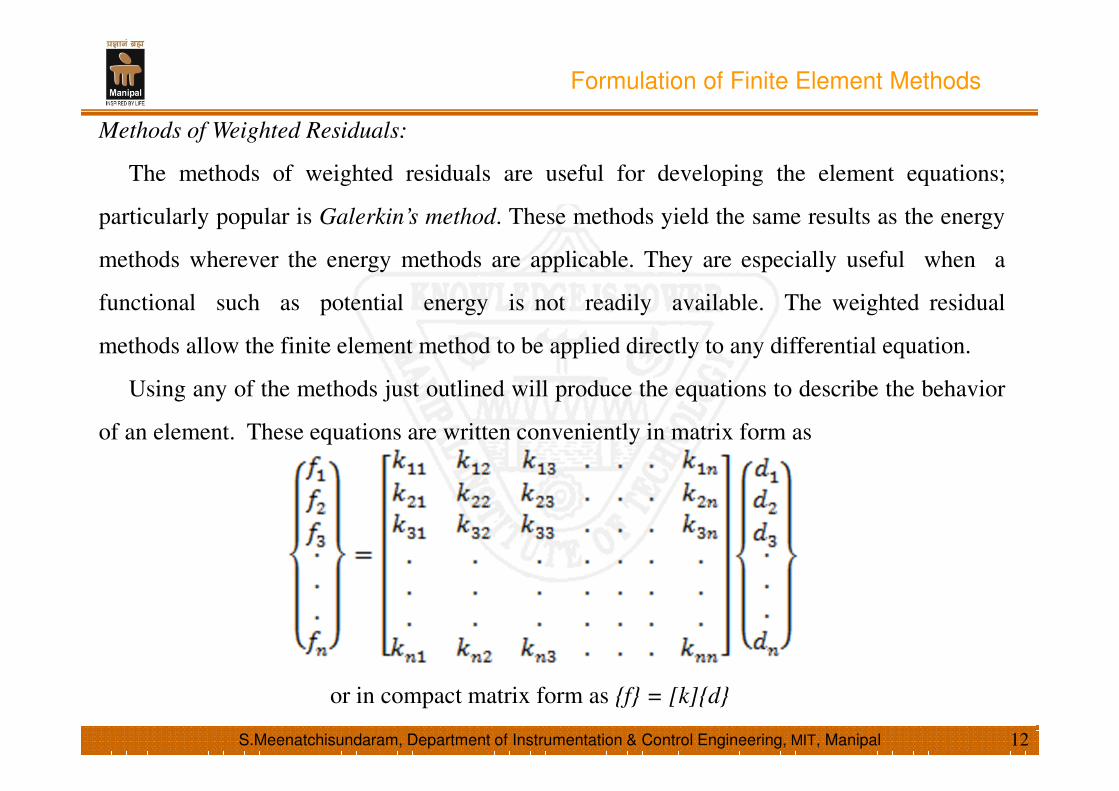
Methods of Weighted Residuals:

The methods of weighted residuals are useful for developing the element equations;

particularly popular is Galerkin’s method. These methods yield the same results as the energy

methods wherever the energy methods are applicable. They are especially useful when a

functional such as potential energy is not readily available. The weighted residual

methods allow the finite element method to be applied directly to any differential equation.

Using any of the methods just outlined will produce the equations to describe the behavior

of an element. These equations are written conveniently in matrix form as

or in compact matrix form as {f} = [k]{d}



Step 5: Assembly the Element Equations to Obtain the Global or Total Equations and

Introduce Boundary Conditions:

The individual element nodal equilibrium equations generated in step 4 are assembled into

the global nodal equilibrium equations. Another more direct method of superposition (called

the direct stiffness method), whose basis is nodal force equilibrium, can be used to obtain the

global equations for the whole structure.

Implicit in the direct stiffness method is the concept of continuity, or compatibility, which

requires that the structure remain together and that no tears occur anywhere within the

structure. The final assembled or global equation written in matrix form is

{F} = [K]{d} (1.4)



Step 6: Solve for the Unknown Degrees of Freedom (or Generalized Displacements):

Equation (1.4), modified to account for the boundary conditions, is a set of simultaneous

algebraic equations that can be written in expanded matrix form as

(1.5)

where now n is the structure total number of unknown nodal degrees of freedom. These

equations can be solved for the ds by using an elimination method (such as Gauss's method)

or an iterative method (such as the Gauss-Seidel method). The ds are called the primary

unknowns, because they are the first quantities determined using the stiffness (or

displacement) finite element method.



Step 7: Solve for the Element Strains and Stresses:

For the structural stress-analysis problem, important secondary quantities of strain and

stress (or moment and shear force) can be obtained because they can be directly expressed in

terms of the displacements determined in step 6. Typical relationships between strain and

displacement and between stress and strain such as Eqs.(1.1) and (1.2) for one-dimensional

stress given in step 3 can be used.

Step 8: Interpret the Results:

The final goal is to interpret and analyze the results for use in the design/analysis process.

Determination of locations in the structure where large deformations and large stresses occur

is generally important in making design/analysis decisions. Postprocessor computer programs

help the user to interpret the results by displaying them in graphical form.


Applications of the Finite Element Method

The finite element method can be used to analyze both structural and nonstructural problems.

Typical structural areas include

1. Stress analysis, including truss and frame analysis, and stress concentration problems

associated with holes, fillets, or other changes in geometry in a body.

2. Buckling

3. Vibration analysis

Nonstructural problems include

1. Heat transfer

2. Fluid flow, including seepage through porous media

3. Distribution of electric or magnetic potential

Some biomechanical engineering problems typically include analyses of human spine, skull,

hip joints, jaw/gum tooth implants, heart, and eye. FEM can also be applied to micro electro

mechanical systems to carry out the Heat Transfer Analysis, Thermal stress analysis, Thermal

Fatigue Stress Analysis, Static Analysis, and Modal Analysis, etc.


Advantages of the Finite Element Method

The finite element method has been applied to numerous problems, both structural and non

structural. This method has a number of advantages that have made it very popular. They

include the ability to

1. Model irregularly shaped bodies quite easily

2. Handle general load conditions without difficult

3. Model bodies composed of several different materials because the element equations

are evaluated individually

4. Handle unlimited numbers and kinds of boundary conditions

5. Vary the size of the elements to make it possible to use small elements where

necessary

6. Alter the finite element model relatively easily and cheaply

7. Include dynamic effects

8. Handle nonlinear behavior existing with large deformations and nonlinear materials.


Stiffness (Displacement) Method

Definition of the Stiffness Matrix:



Derivation of the Stiffness Matrix for a Spring Element:



Example Problem :

For the spring assemblage with arbitrarily numbered nodes shown in Figure, evaluate the

unknown displacements, reaction and element forces. A force of 5000 N is applied at node 2

in the x direction and a force of 10,000 N is applied at node 3 in negative x direction. The

spring constants are k1=1000N/m, k2=2000N/m, k3=3000N/m. Node 1 and node 4 are fixed.
