Mass transfer

Jamin Koo

2019. 11. 4

Lecture 11: Diffusion

1

Learning objectives

2

• Be able to apply Fick’s first law in analyzing mass transfer during equimolar and one-way diffusion.

• Have both qualitative and quantitative knowledge of diffusion by gases and liquids, especially with respect to diffusivities.

• Have practical understanding of Schmidt number.

Today’s outline

3

• Background Introduction

Four types of situations

Fick’s first law, and molar flowrate

Equimolar diffusion

One-way diffusion

• Diffusivities and Schmidt number Relations between diffusivities

Diffusion of gases, experimental values

Diffusion of liquids

Schmidt number

• Convection versus diffusion

https://www.youtube.com/watch?v=EG4ZoVTSA5I&t=9s

4

17.1 Introduction

5

• Diffusion can be due to gradient in many conditions including concentration, temperature, pressure, activity, and external force. We will only consider diffusion due to concentration

gradient in this chapter.

Why does molecules diffuse from higher concentration to a lower concentration?

17.1 Four types of situations

6

• Mass transfer through diffusion results in one of the following 4 types of situations:

1) Only one component A of the mixture is transferred

2) Diffusion of A is balanced by opposite molar flow of B, resulting in zero net molar flow.

3) Diffusion of A and B occur in opposite directions with unequal amounts.

4) Two or more components diffuse in the same direction but at different rates.

17.1 Fick’s first law

7

• For steady state, 1D diffusion in a direction perpendicular to the interface,

𝐽𝐴 = −𝐷𝑣d𝑐𝐴

d𝑏

where 𝐽𝐴 is the molar flux [mol/m2/hr],

𝐷𝑣 is the volumetric diffusivity [m2/hr]

𝑐𝐴 is the concentration of A [mol/m3]

b is the distance in the direction of diffusion [m]

For 3D diffusion,

𝐽𝐴 = −𝐷𝑣 𝛻𝑐𝐴 = −𝜌𝑀 𝐷𝑣 𝛻𝑥𝐴where 𝜌𝑀 is the molar density of the mixture [mol/m3]

𝑥𝐴 is the mole fraction of A

17.1 Molar flow rate

8

• For components A and B crossing a stationary plane, the molar fluxes are

𝑁𝒊 = 𝑐𝑖 𝑢𝑖

where ui is the volumetric average velocity [m/hr] of component i

• For a reference plane moving at the volume-average velocity u0, There is no net volumetric flow across this plane.

The molar flux of A through this reference plane becomes

𝐽𝐴 = 𝑐𝐴 𝑢𝐴 − 𝑐𝐴 𝑢0 = 𝑐𝐴(𝑢𝐴 − 𝑢0) = −𝐷𝐴𝐵d𝑐𝐴

d𝑏

𝑁𝐴 = 𝑐𝐴 𝑢0 + −𝐷𝐴𝐵d𝑐𝐴

d𝑏

where DAB is the diffusivity of A in its mixture with B.

The diffusion velocity is relative to volume-average velocity 𝑢0.

17.1 Equimolal diffusion

9

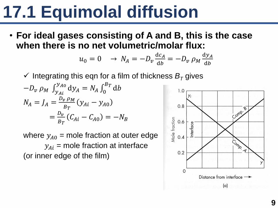
• For ideal gases consisting of A and B, this is the case when there is no net volumetric/molar flux:

𝑢0 = 0 → 𝑁𝐴 = −𝐷𝑣d𝑐𝐴

d𝑏= −𝐷𝑣 𝜌𝑀

d𝑦𝐴

d𝑏

Integrating this eqn for a film of thickness BT gives

−𝐷𝑣 𝜌𝑀 𝑦𝐴𝑖

𝑦𝐴0 d𝑦𝐴 = 𝑁𝐴 0𝐵𝑇 d𝑏

𝑁𝐴 = 𝐽𝐴 =𝐷𝑣 𝜌𝑀

𝐵𝑇𝑦𝐴𝑖 − 𝑦𝐴0

=𝐷𝑣

𝐵𝑇𝐶𝐴𝑖 − 𝐶𝐴0 = −𝑁𝐵

where 𝑦𝐴0 = mole fraction at outer edge

𝑦𝐴𝑖 = mole fraction at interface

(or inner edge of the film)

17.1 One-way diffusion

10

• For ideal gases consisting of A and B, this is the case when only component A is being transferred:

𝑁 = 𝑁𝐴 → 𝑁𝐴 = 𝑦𝐴 𝑁𝐴 − 𝐷𝑣 𝜌𝑀d𝑦𝐴

d𝑏

Rearranging and integrating this eqn for a film of thickness BT gives

−𝐷𝑣 𝜌𝑀 𝑦𝐴𝑖

𝑦𝐴0 1

1−𝑦𝐴d𝑦𝐴 = 𝑁𝐴 0

𝐵𝑇 d𝑏

𝑁𝐴 =𝐷𝑣 𝜌𝑀

𝐵𝑇ln

1−𝑦𝐴0

1−𝑦𝐴𝑖

=𝐷𝑣 𝜌𝑀

𝐵𝑇

𝑦𝐴𝑖−𝑦𝐴0

(1−𝑦𝐴)𝐿

where (1 − 𝑦𝐴)𝐿 =𝑦𝐴𝑖−𝑦𝐴0

ln1−𝑦𝐴01−𝑦𝐴𝑖

For a given 𝑦𝐴𝑖 − 𝑦𝐴0, is one-way

diffusion faster or slower than the

equilmolar diffusion?

17.1 Relations between diffusivities

11

• For ideal gases consisting of A and B,

𝑐𝐴 + 𝑐𝐵 = 𝜌𝑀 =𝑃

𝑅 𝑇[mol/m3]

where R is the ideal gas constant; P and T are pressure and temp.

At constant T & P, the mixture density remains constant, meaningd𝜌𝑀 = d𝑐𝐴 + d𝑐𝐵 = 0

−𝐷𝐴𝐵d𝑐𝐴

d𝑏− 𝐷𝐵𝐴

d𝑐𝐵

d𝑏= 0 → 𝐷𝐴𝐵 = 𝐷𝐵𝐴

• For liquid mixture of A and B, 𝑐𝐴 𝑀𝐴 + 𝑐𝐵 𝑀𝐵 = 𝜌 = 𝑐𝑜𝑛𝑠𝑡𝑎𝑛𝑡 [kg/m3]

where Mi is the molecular weight of a component i.

If all mixtures have the same 𝜌, d𝜌 = 𝑀𝐴 d𝑐𝐴 + 𝑀𝐵 d𝑐𝐵 = 0

−𝐷𝐴𝐵d𝑐𝐴

d𝑏

𝑀𝐴

𝜌− 𝐷𝐵𝐴

d𝑐𝐵

d𝑏

𝑀𝐵

𝜌= 0 → 𝐷𝐴𝐵 = 𝐷𝐵𝐴

17.1 Diffusion of gases

12

• Simple theory states

𝐷𝑣 ≅1

3 𝑢 𝜆

where 𝑢 and 𝜆 are the average molecular velocity and mean free path.

• Using the modern kinetic theory,

𝐷𝐴𝐵 =0.001858 𝑇3/2 [(𝑀𝐴+𝑀𝐵)/𝑀𝐴 𝑀𝐵]1/2

𝑃 𝜎𝐴𝐵2 𝛺𝐷

where 𝜎𝐴𝐵 and 𝛺𝐷 are effective collision diameter and integral, respectively.

• When diffusing through a cylindrical pore (D << 𝜆),

𝐷𝐾 = 9,700 𝑟 𝑇/𝑀

where 𝐷𝐾 = Knudsen diffusivity [cm2/s], r = pore radium [cm],

T = temp. [K], and M = molecular weight [g/mol]

17.1 Experimental values

13

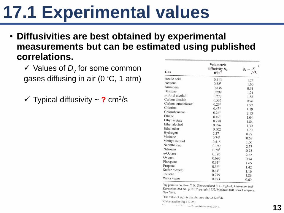
• Diffusivities are best obtained by experimental measurements but can be estimated using published correlations. Values of Dv for some common

gases diffusing in air (0 ◦C, 1 atm)

Typical diffusivity ~ ? cm2/s

17.1 Diffusion of liquids

14

• Limited experimental data and models are available. Diffusivities are usually 104~105 lower than gases at 1 atm. Why?

Fluxes for a given mole fraction, however, is similar to gases. Why?

• For large spherical molecules in dilute solution,

𝐷𝑣 =𝑘 𝑇

6𝜋 𝑟0 𝜇=

7.32 × 10−16 𝑇

𝑟0 𝜇[cm2/s]

where 𝑟0 is the molecular radius [cm], 𝜇 is viscosity [cP], and k is ???

• For small to moderate molecules (MW < 400 g/mole),

𝐷𝑣 = 7.4 × 10−8 (𝜓𝐵 𝑀𝐵)1/2 𝑇

𝜇 𝑉𝐴0.6 [cm2/s]

where 𝜓𝐵 and 𝑉𝐴 are association parameter for solvent, and molar volume of solute as liquid at its normal bp, respectively.

17.1 Diffusion of liquids

15

• For dilute aqueous solutions of non-electrolytes,

𝐷𝑣 =13.26 × 10−5

𝜇𝐵1.14 𝑉𝐴

0.589 [cm2/s]

where 𝜇B is viscosity of water [cP].

• For dilute solutions of completely ionized univalent electrolytes,

𝐷𝑣 =2𝑅 𝑇

(1

𝜆+0+

1

𝜆−0) 𝐹𝑎

2[cm2/s]

where 𝜆+0 and 𝜆−

0 are limiting (zero-concentration) ionic conductance [A cm2

/V/g]; Fa is Faraday constant (96,500 C/g].

• Is diffusivity the same for the same liquid? Why or why not?

17.1 Schmidt number

16

• It is the ratio of kinematic viscosity to the diffusivity:

𝑆𝑐 =𝜐

𝐷𝑣=

𝜇

𝜌 𝐷𝑣

For gases in air (0 ◦C, 1 atm), it is about 0.2~3.0.

For liquids, it ranges from 102 to 105 for typical mixtures: 𝐷𝑣 ~ 10-5

cm2/s and Sc ~ 103 for small solutes in water (20 ◦C).

What would happen, for liquids, if T increases?