lecture 11: networks ii: conductance-based synapses, visual cortical hypercolumn model
DESCRIPTION
Lecture 11: Networks II: conductance-based synapses, visual cortical hypercolumn model. References: Hertz, Lerchner, Ahmadi, q-bio.NC/0402023 [Erice lectures] Lerchner, Ahmadi, Hertz, q-bio.NC/0402026 (Neurocomputing, 2004) [conductance-based synapses] - PowerPoint PPT PresentationTRANSCRIPT
Lecture 11: Networks II:conductance-based synapses,
visual cortical hypercolumn model
References:Hertz, Lerchner, Ahmadi, q-bio.NC/0402023 [Erice lectures]Lerchner, Ahmadi, Hertz, q-bio.NC/0402026
(Neurocomputing, 2004) [conductance-based synapses]Lerchner, Sterner, Hertz, Ahmadi, q-bio.NC/0403037
[orientation hypercolumn model]

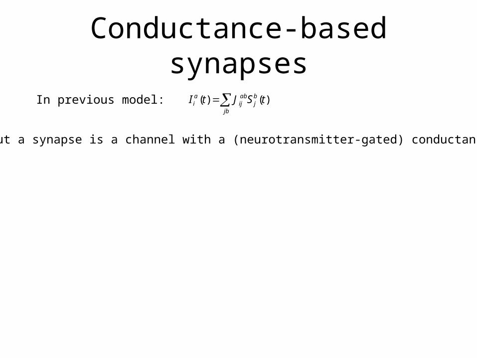
Conductance-based synapses
In previous model: )()( tSJtI bj
jb
abij
ai
Conductance-based synapses
In previous model: )()( tSJtI bj
jb
abij
ai
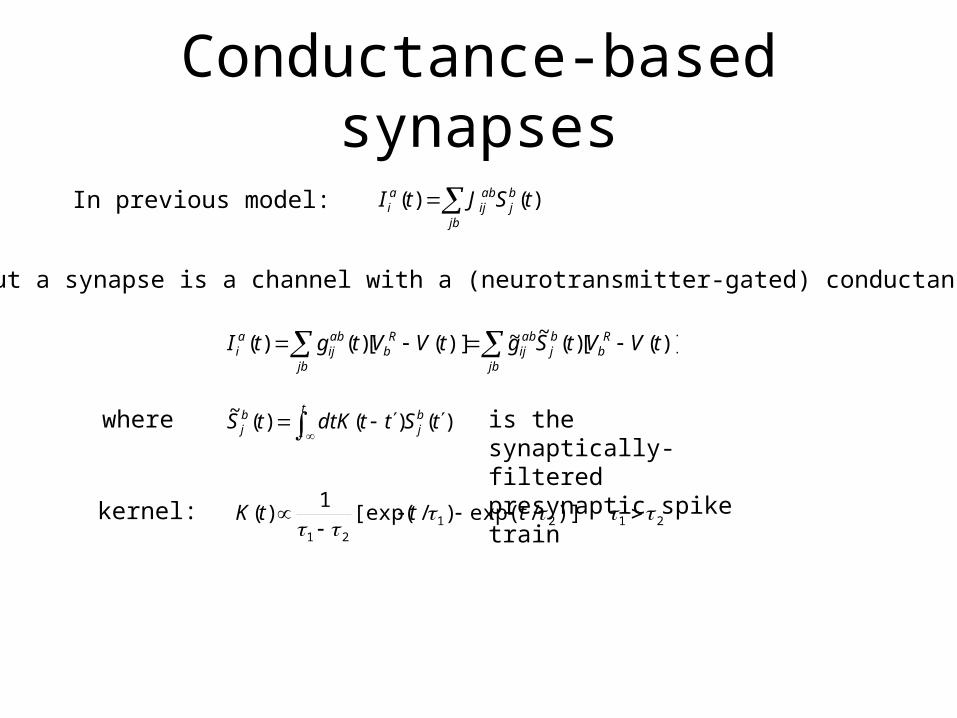
But a synapse is a channel with a (neurotransmitter-gated) conductance:

Conductance-based synapses
In previous model: )()( tSJtI bj
jb
abij
ai
But a synapse is a channel with a (neurotransmitter-gated) conductance:
)]([)(~~)]([)()( tVVtSgtVVtgtI Rb
jb
bj
abij
Rb
jb
abij
ai

Conductance-based synapses
In previous model: )()( tSJtI bj
jb
abij
ai
But a synapse is a channel with a (neurotransmitter-gated) conductance:
)]([)(~~)]([)()( tVVtSgtVVtgtI Rb
jb
bj
abij
Rb
jb
abij
ai
where
t bj
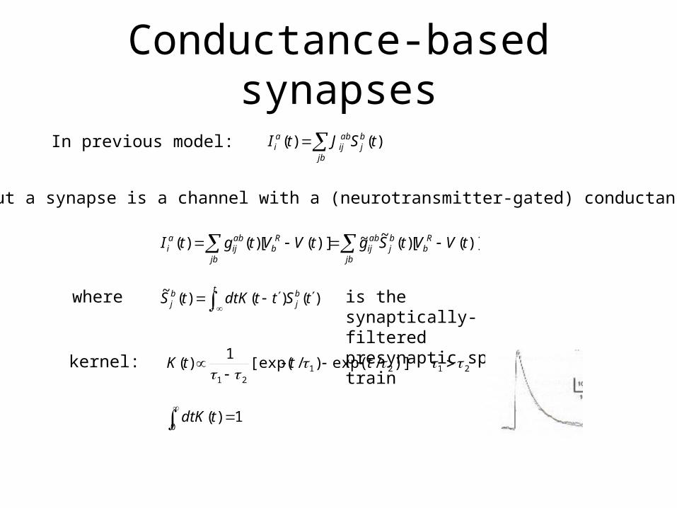
bj tSttKdttS )()()(~ is the synaptically-filtered
presynaptic spike train
Conductance-based synapses
In previous model: )()( tSJtI bj
jb
abij
ai
But a synapse is a channel with a (neurotransmitter-gated) conductance:
)]([)(~~)]([)()( tVVtSgtVVtgtI Rb
jb
bj
abij
Rb
jb
abij
ai
where
t bj
bj tSttKdttS )()()(~ is the synaptically-filtered
presynaptic spike train
212121
)]/exp()/[exp(1
)(
tttKkernel:
Conductance-based synapses
In previous model: )()( tSJtI bj
jb
abij
ai
But a synapse is a channel with a (neurotransmitter-gated) conductance:
)]([)(~~)]([)()( tVVtSgtVVtgtI Rb
jb
bj
abij
Rb
jb
abij
ai
where
t bj
bj tSttKdttS )()()(~ is the synaptically-filtered
presynaptic spike train
0
1)(tKdt
212121
)]/exp()/[exp(1
)(
tttKkernel:

Model

Model
b
babij
b
b
b
ababij N
Kg
N
K
K
gg 1 prob,0~;prob,~
0

Model
b
babij
b
b
b
ababij N
Kg
N
K
K
gg 1 prob,0~;prob,~
0
)()(~~)(
))(()(
0
2
0,0
Rb
ai
jb
bj
abij
Rleak
ai
bj
Rb
ai
abij
Rleak
ai
ai
VVtSgVVg
VVtgVVgdt
dV

Mean field theoryEffective single-neuron problem with synaptic input current

Mean field theory
aR
bb
ababb
b
bbbab
ba
Rbaba
VVtxqNK
rKg
VVtgtI
)(1
)()(
2/1
0
Effective single-neuron problem with synaptic input current

Mean field theory
aR
bb
ababb
b
bbbab
ba
Rbaba
VVtxqNK
rKg
VVtgtI
)(1
)()(
2/1
0
Effective single-neuron problem with synaptic input current
1)(,0 2 abab xx
)()()(,0)( ttCttt bababab
with 2)( bjb rq

Mean field theory
aR
bb
ababb
b
bbbab
ba
Rbaba
VVtxqNK
rKg
VVtgtI
)(1
)()(
2/1
0
Effective single-neuron problem with synaptic input current
1)(,0 2 abab xx
)()()(,0)( ttCttt bababab
with
where
t t
bbj
bjb ttCttKdtttKdttStSttC )()()()(~)(~)( 212211
= correlation function of synaptically-filtered presynaptic spike trains
2)( bjb rq

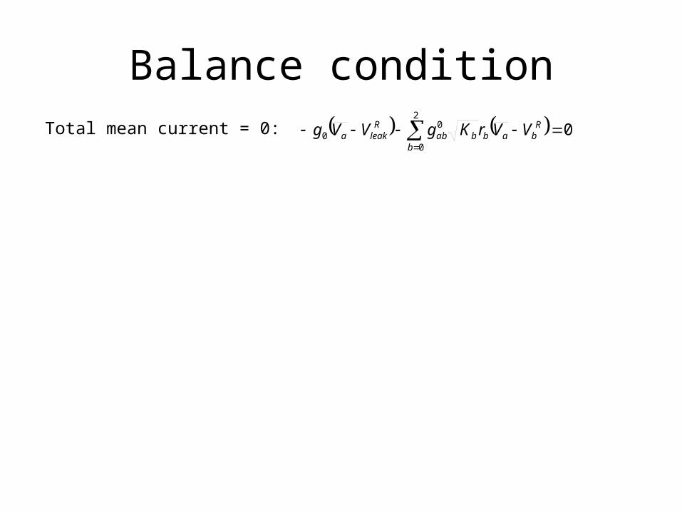
Balance conditionTotal mean current = 0:
Balance condition 0
2
0
00
b
Rbabbab
Rleaka VVrKgVVgTotal mean current = 0:

Balance condition 0
2
0
00
b
Rbabbab
Rleaka VVrKgVVg
aV
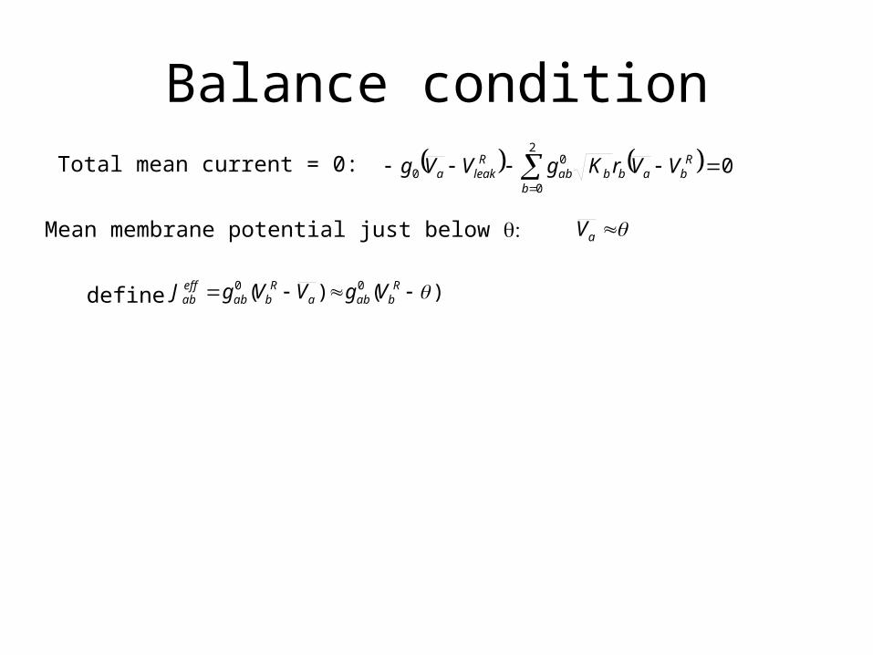
Total mean current = 0:
Mean membrane potential just below
Balance condition 0
2
0
00
b
Rbabbab
Rleaka VVrKgVVg
define )()( 00 Rbaba
Rbab
effab VgVVgJ
aV
Total mean current = 0:
Mean membrane potential just below

Balance condition 0
2
0
00
b
Rbabbab
Rleaka VVrKgVVg
define )()( 00 Rbaba
Rbab
effab VgVVgJ 02 eff
aJ
aV
Total mean current = 0:
Mean membrane potential just below

Balance condition 0
2
0
00
b
Rbabbab
Rleaka VVrKgVVg
define )()( 00 Rbaba
Rbab
effab VgVVgJ
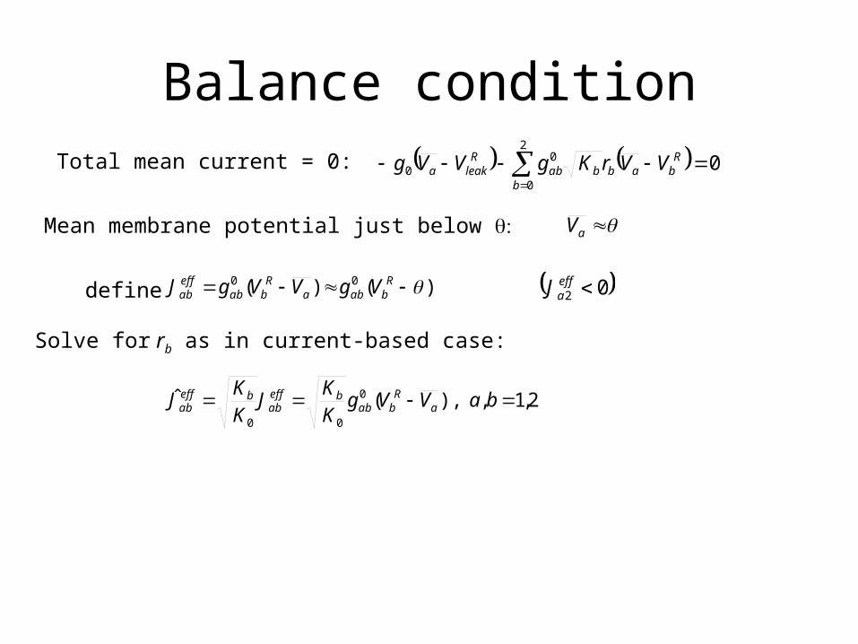
Solve for rb as in current-based case:
02 effaJ
aV
Total mean current = 0:
Mean membrane potential just below
Balance condition 0
2
0
00
b
Rbabbab
Rleaka VVrKgVVg
define )()( 00 Rbaba
Rbab
effab VgVVgJ
Solve for rb as in current-based case:
2,1,),(ˆ 0
00
baVVgK
KJ
K
KJ a
Rbab
beffab
beffab
02 effaJ
aV
Total mean current = 0:
Mean membrane potential just below

Balance condition 0
2
0
00
b
Rbabbab
Rleaka VVrKgVVg
define )()( 00 Rbaba
Rbab
effab VgVVgJ
Solve for rb as in current-based case:
2,1,),(ˆ 0
00
baVVgK
KJ
K
KJ a
Rbab
beffab
beffab
))((
))((
ˆˆ
ˆˆ
)(
)(02
020
)(
)(01
010
1
2221
1211
2
1
20200
20
10100
10
VVgK
VVgRex
VVgK
VVgRex
effeff
effeff
Rex
Rleak
Rex
Rleak
rVVg
rVVg
JJ
JJ
r
r
02 effaJ
aV
Total mean current = 0:
Mean membrane potential just below
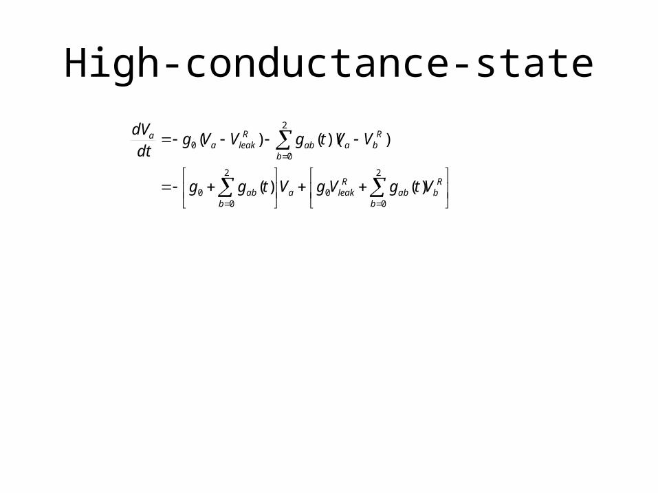
High-conductance-state
2
00
2
00
2
00
)()(
))(()(
b
Rbab
Rleaka
bab
b
Rbaab
Rleaka
a
VtgVgVtgg
VVtgVVgdt
dV

High-conductance-state
2
00
2
00
2
00
)()(
))(()(
b
Rbab
Rleaka
bab
b
Rbaab
Rleaka
a
VtgVgVtgg
VVtgVVgdt
dV
)]()[()(
)()(
0
0
0 tVVtgtgg
VtgVgVtgg a
satot
bab
b
Rbab
Rleak
ab
ab

High-conductance-state
2
00
2
00
2
00
)()(
))(()(
b
Rbab
Rleaka
bab
b
Rbaab
Rleaka
a
VtgVgVtgg
VVtgVVgdt
dV
)]()[()(
)()(
0
0
0 tVVtgtgg
VtgVgVtgg a
satot
bab
b
Rbab
Rleak
ab
ab
Va “chases” Vsa(t) at rate gtot(t)

High-conductance-state
2
00
2
00
2
00
)()(
))(()(
b
Rbab
Rleaka
bab
b
Rbaab
Rleaka
a
VtgVgVtgg
VVtgVVgdt
dV
)]()[()(
)()(
0
0
0 tVVtgtgg
VtgVgVtgg a
satot
bab
b
Rbab
Rleak
ab
ab
Va “chases” Vsa(t) at rate gtot(t)
mtot gg
1
0

High-conductance-state
2
00
2
00
2
00
)()(
))(()(
b
Rbab
Rleaka
bab
b
Rbaab
Rleaka
a
VtgVgVtgg
VVtgVVgdt
dV
)]()[()(
)()(
0
0
0 tVVtgtgg
VtgVgVtgg a
satot
bab
b
Rbab
Rleak
ab
ab
Va “chases” Vsa(t) at rate gtot(t)
mtot gg
1
0 meffm

High-conductance-state
2
00
2
00
2
00
)()(
))(()(
b
Rbab
Rleaka
bab
b
Rbaab
Rleaka
a
VtgVgVtgg
VVtgVVgdt
dV
)]()[()(
)()(
0
0
0 tVVtgtgg
VtgVgVtgg a
satot
bab
b
Rbab
Rleak
ab
ab
Va “chases” Vsa(t) at rate gtot(t)
mtot gg
1
0 meffm
Effective membrane time constant ~ 1 ms

Membrane potential and spiking dynamics for large gtot

FluctuationsMeasure membrane potential from :aV

FluctuationsMeasure membrane potential from :aV aaa uVV
FluctuationsMeasure membrane potential from :aV aaa uVV
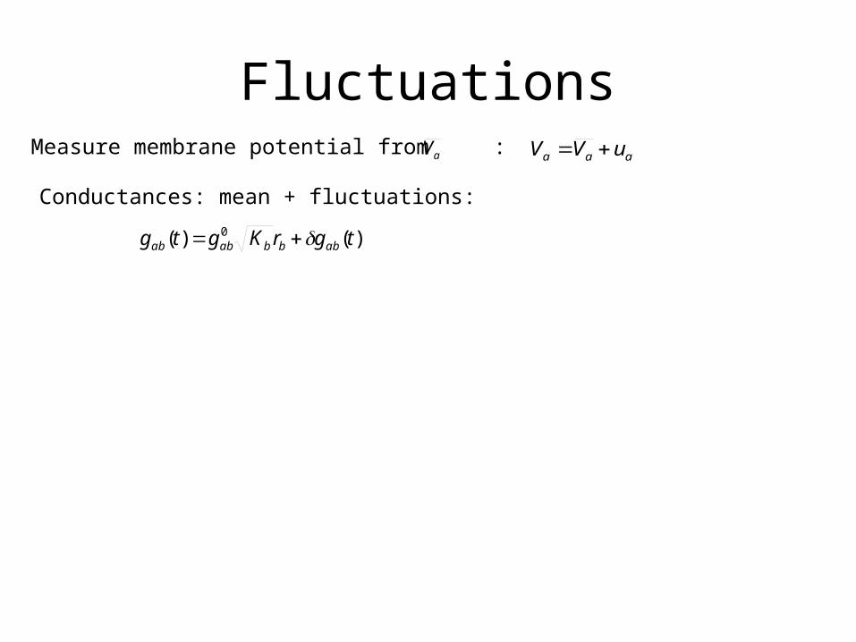
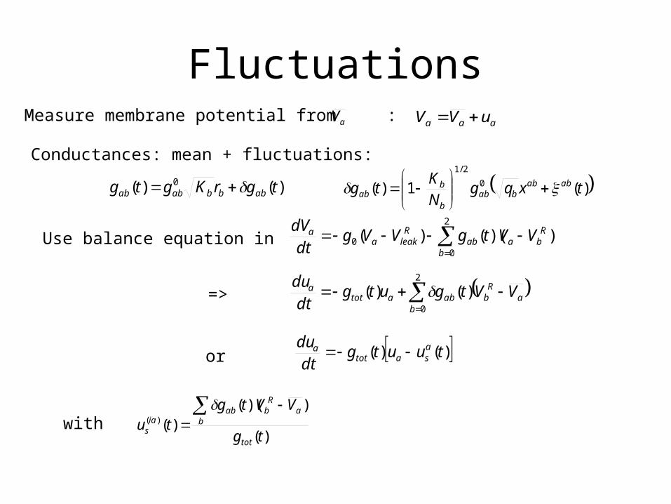
Conductances: mean + fluctuations:
FluctuationsMeasure membrane potential from :aV aaa uVV
Conductances: mean + fluctuations:
)()( 0 tgrKgtg abbbabab

FluctuationsMeasure membrane potential from :aV aaa uVV
Conductances: mean + fluctuations:
)()( 0 tgrKgtg abbbabab )(1)( 0
2/1
txqgNK
tg ababbab
b
bab

FluctuationsMeasure membrane potential from :aV aaa uVV
Use balance equation in
Conductances: mean + fluctuations:
2
00 ))(()(
b
Rbaab
Rleaka
a VVtgVVgdt
dV
)()( 0 tgrKgtg abbbabab )(1)( 0
2/1
txqgNK
tg ababbab
b
bab

FluctuationsMeasure membrane potential from :aV aaa uVV
Use balance equation in
2
0
)()(b
aR
babatota VVtgutg
dt
du
Conductances: mean + fluctuations:
2
00 ))(()(
b
Rbaab
Rleaka
a VVtgVVgdt
dV
=>
)()( 0 tgrKgtg abbbabab )(1)( 0
2/1
txqgNK
tg ababbab
b
bab

FluctuationsMeasure membrane potential from :aV aaa uVV
Use balance equation in
2
0
)()(b
aR
babatota VVtgutg
dt
du
Conductances: mean + fluctuations:
2
00 ))(()(
b
Rbaab
Rleaka
a VVtgVVgdt
dV
=>
or )()( tuutgdt
du asatot
a
)()( 0 tgrKgtg abbbabab )(1)( 0
2/1
txqgNK
tg ababbab
b
bab
FluctuationsMeasure membrane potential from :aV aaa uVV
Use balance equation in
2
0
)()(b
aR
babatota VVtgutg
dt
du
Conductances: mean + fluctuations:
2
00 ))(()(
b
Rbaab
Rleaka
a VVtgVVgdt
dV
=>
or )()( tuutgdt
du asatot
a
)()( 0 tgrKgtg abbbabab
with)(
))(()()(
tg
VVtgtu
tot
ba
Rbab
ias
)(1)( 0
2/1
txqgNK
tg ababbab
b
bab

FluctuationsMeasure membrane potential from :aV aaa uVV
Use balance equation in
2
0
)()(b
aR
babatota VVtgutg
dt
du
Conductances: mean + fluctuations:
2
00 ))(()(
b
Rbaab
Rleaka
a VVtgVVgdt
dV
=>
or )()( tuutgdt
du asatot
a
)()( 0 tgrKgtg abbbabab
with)(
))(()()(
tg
VVtgtu
tot
ba
Rbab
ias
b babbbabtot tgrKggtg )()( 0
0
)(1)( 0
2/1
txqgNK
tg ababbab
b
bab
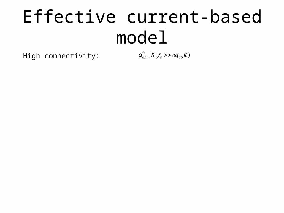
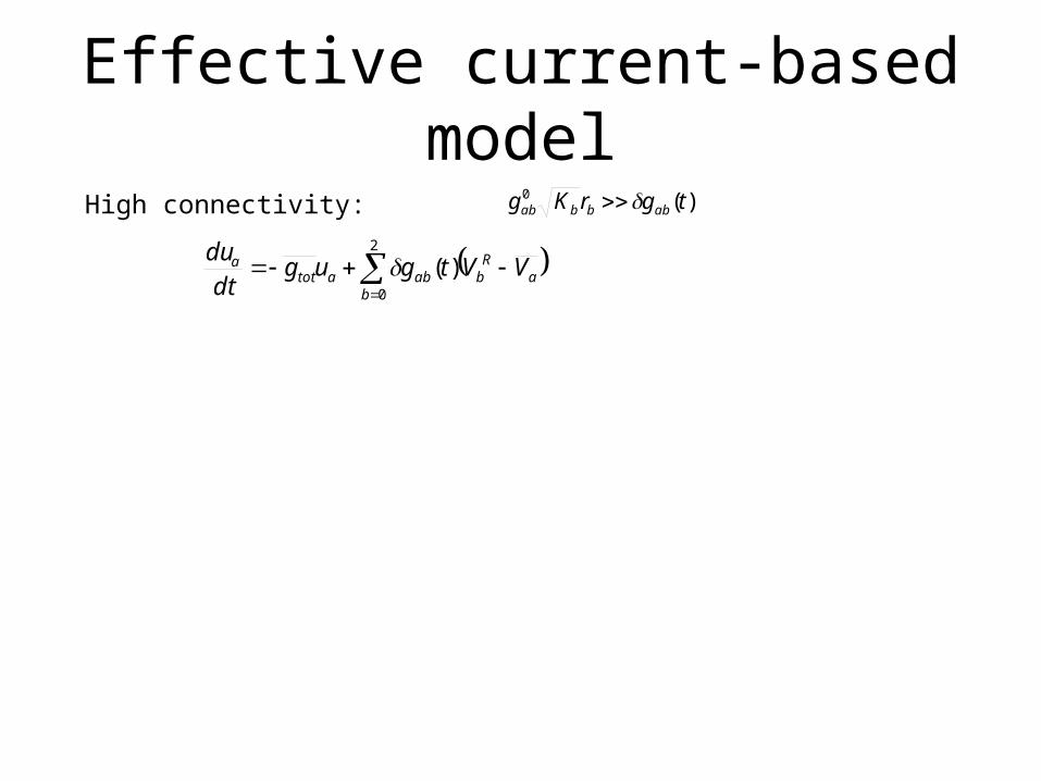
Effective current-based model)(0 tgrKg abbbab High connectivity:
Effective current-based model)(0 tgrKg abbbab
2
0
)(b
aR
babatota VVtgug
dtdu
High connectivity:

Effective current-based model)(0 tgrKg abbbab
2
0
)(b
aR
babatota VVtgug
dtdu
High connectivity:
)()(1 0
2/1
ba
Rb
ababbab
b
batot VVtxqg
NK
ug

Effective current-based model)(0 tgrKg abbbab
2
0
)(b
aR
babatota VVtgug
dtdu
High connectivity:
)()(1 0
2/1
ba
Rb
ababbab
b
batot VVtxqg
NK
ug
b
ababb
effab
b
batot txqJ
NK
ug )(12/1

Effective current-based model)(0 tgrKg abbbab
b
bbabtot rKggg 00
2
0
)(b
aR
babatota VVtgug
dtdu
High connectivity:
)()(1 0
2/1
ba
Rb
ababbab
b
batot VVtxqg
NK
ug
b
ababb
effab
b
batot txqJ
NK
ug )(12/1

Effective current-based model)(0 tgrKg abbbab
b
bbabtot rKggg 00
2
0
)(b
aR
babatota VVtgug
dtdu
High connectivity:
)()(1 0
2/1
ba
Rb
ababbab
b
batot VVtxqg
NK
ug
b
ababb
effab
b
batot txqJ
NK
ug )(12/1
Like current-based model with toteffmm
eff g/1; JJ

Effective current-based model)(0 tgrKg abbbab
b
bbabtot rKggg 00
2
0
)(b
aR
babatota VVtgug
dtdu
High connectivity:
)()(1 0
2/1
ba
Rb
ababbab
b
batot VVtxqg
NK
ug
b
ababb
effab
b
batot txqJ
NK
ug )(12/1
Like current-based model with toteffmm
eff g/1; JJ
(but effective membrane time constant depends onpresynaptic rates)

Firing irregularity depends on reset level and s

Modeling primary visual cortex

Modeling primary visual cortex
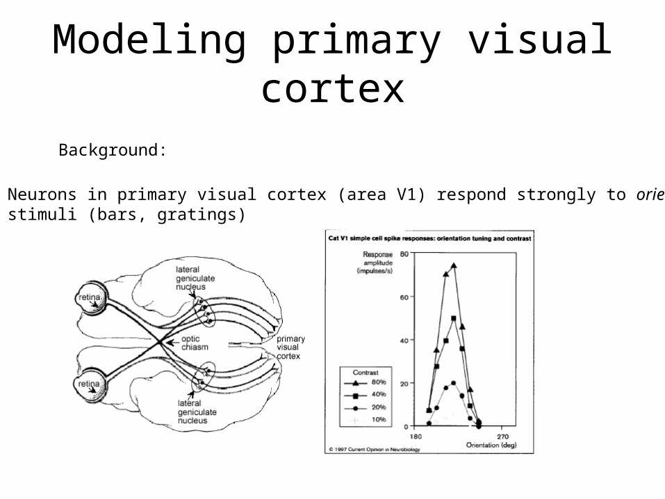
Background:
1. Neurons in primary visual cortex (area V1) respond strongly to oriented stimuli (bars, gratings)
Modeling primary visual cortex
Background:
1. Neurons in primary visual cortex (area V1) respond strongly to oriented stimuli (bars, gratings)

Modeling primary visual cortex
Background:
1. Neurons in primary visual cortex (area V1) respond strongly to oriented stimuli (bars, gratings)
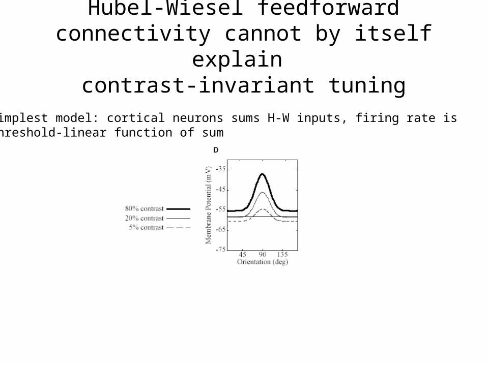
Note:contrast-invarianttuning width

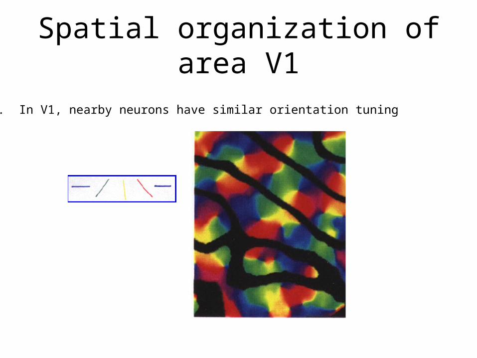
Spatial organization of area V1
2. In V1, nearby neurons have similar orientation tuning
Spatial organization of area V1
2. In V1, nearby neurons have similar orientation tuning

Orientation column~ 104 neurons that respond most strongly to a particular orientation

Orientation column~ 104 neurons that respond most strongly to a particular orientation
Tuning of input from LGN (Hubel-Wiesel):
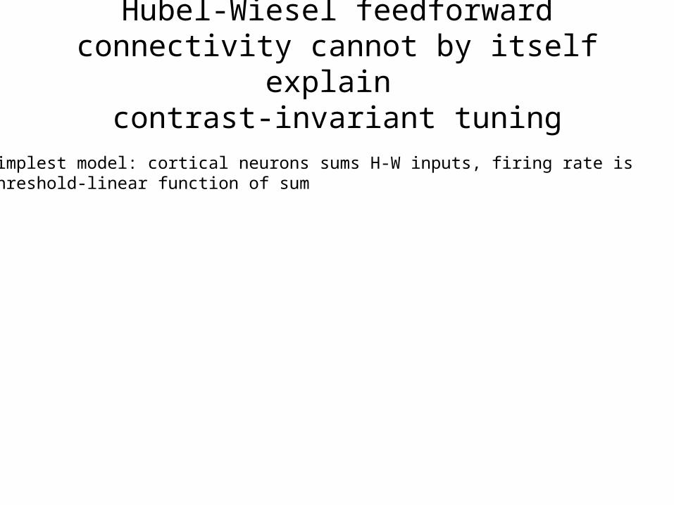
Hubel-Wiesel feedforward connectivity cannot by itself explain contrast-invariant tuning
Simplest model: cortical neurons sums H-W inputs, firing rate isthreshold-linear function of sum
Hubel-Wiesel feedforward connectivity cannot by itself explain contrast-invariant tuning
Simplest model: cortical neurons sums H-W inputs, firing rate isthreshold-linear function of sum
Modeling a “hypercolumn” in V1
Coupled collection of networks, each representing an “orientation column”

Modeling a “hypercolumn” in V1
Coupled collection of networks, each representing an “orientation column”

Modeling a “hypercolumn” in V1
Coupled collection of networks, each representing an “orientation column”
2
1 1
/
1
,00 )()(
b
n nN
j
bj
baija
ai
ai
b
tSJIV
dtdV

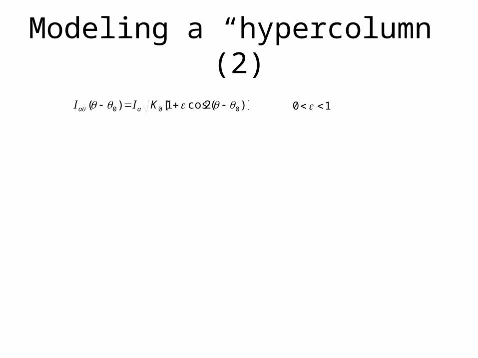
Modeling a “hypercolumn” (2)
)](2cos1[)( 000 KII aa
Modeling a “hypercolumn” (2)
)](2cos1[)( 000 KII aa 10
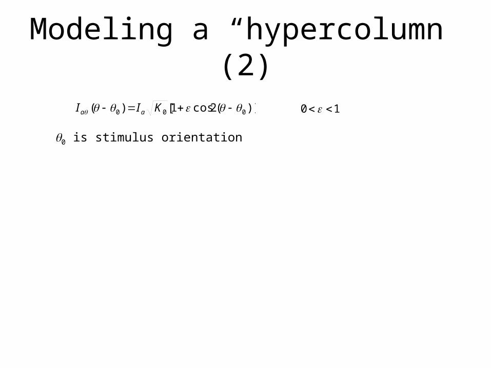
Modeling a “hypercolumn” (2)
)](2cos1[)( 000 KII aa
0 is stimulus orientation
10

Modeling a “hypercolumn” (2)
)](2cos1[)( 000 KII aa
0 is stimulus orientation
10
(simplest model periodic in with period )

Modeling a “hypercolumn” (2)
)](2cos1[1 prob,0
)](2cos1[prob,
,
,
b
bbaij
b
b
b
abbaij
NK
J
NK
K
JJ
)](2cos1[)( 000 KII aa
0 is stimulus orientation
10
(simplest model periodic in with period )

Modeling a “hypercolumn” (2)
)](2cos1[1 prob,0
)](2cos1[prob,
,
,
b
bbaij
b
b
b
abbaij
NK
J
NK
K
JJ
)](2cos1[)( 000 KII aa
0 is stimulus orientation
10
2,0 bJab
10
(simplest model periodic in with period )

Modeling a “hypercolumn” (2)
)](2cos1[1 prob,0
)](2cos1[prob,
,
,
b
bbaij
b
b
b
abbaij
NK
J
NK
K
JJ
)](2cos1[)( 000 KII aa
0 is stimulus orientation
10
2,0 bJab
Connection probability falls off with increasing’, reflecting probable greater distance.
10
(simplest model periodic in with period )

Mean field theory
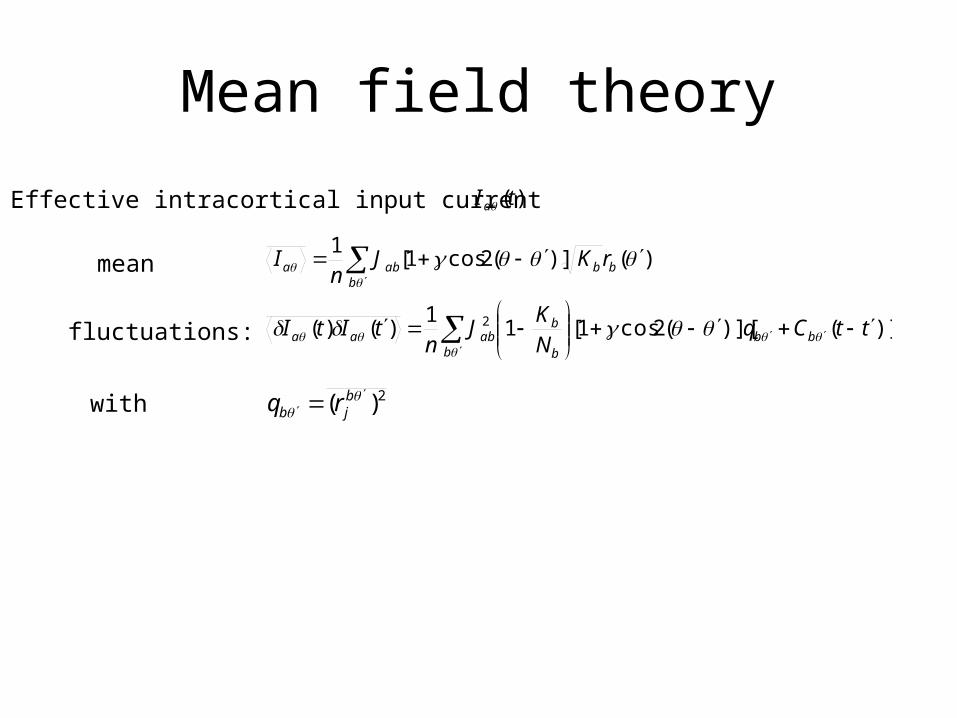
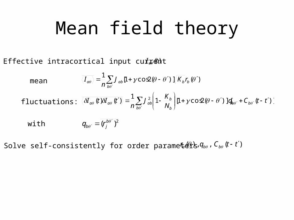
Effective intracortical input current )(tIa

Mean field theory
Effective intracortical input current )(tIa
)()](2cos1[1
bb
baba rKJ
nImean

Mean field theory
Effective intracortical input current )(tIa
)()](2cos1[1
bb
baba rKJ
nImean
)]()][(2cos1[11
)()( 2 ttCqNK
Jn
tItI bbb
b
babaa
fluctuations:
Mean field theory
Effective intracortical input current )(tIa
)()](2cos1[1
bb
baba rKJ
nImean
)]()][(2cos1[11
)()( 2 ttCqNK
Jn
tItI bbb
b
babaa
fluctuations:
2)(
b
jb rqwith
Mean field theory
Effective intracortical input current )(tIa
)()](2cos1[1
bb
baba rKJ
nImean
)]()][(2cos1[11
)()( 2 ttCqNK
Jn
tItI bbb
b
babaa
fluctuations:
2)(
b
jb rqwith
Solve self-consistently for order parameters )(,),( ttCqr bba

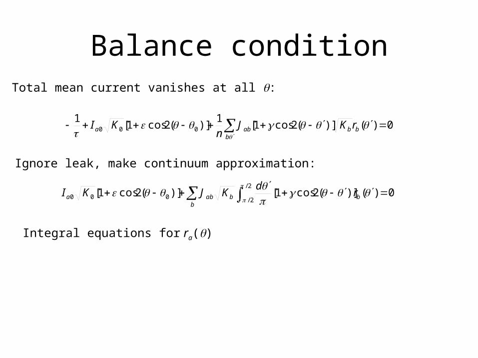
Balance conditionTotal mean current vanishes at all :

Balance conditionTotal mean current vanishes at all :
0)()](2cos1[1
)](2cos1[1
000
bbb
aba rKJn
KI

Balance conditionTotal mean current vanishes at all :
0)()](2cos1[1
)](2cos1[1
000
bbb
aba rKJn
KI
Ignore leak, make continuum approximation:

Balance conditionTotal mean current vanishes at all :
0)()](2cos1[1
)](2cos1[1
000
bbb
aba rKJn
KI
0)()](2cos1[)](2cos1[2/
2/000
b
bbaba r
dKJKI
Ignore leak, make continuum approximation:
Balance conditionTotal mean current vanishes at all :
0)()](2cos1[1
)](2cos1[1
000
bbb
aba rKJn
KI
0)()](2cos1[)](2cos1[2/
2/000
b
bbaba r
dKJKI
Ignore leak, make continuum approximation:
Integral equations for ra()

Balance conditionTotal mean current vanishes at all :
0)()](2cos1[1
)](2cos1[1
000
bbb
aba rKJn
KI
0)()](2cos1[)](2cos1[2/
2/000
b
bbaba r
dKJKI
Ignore leak, make continuum approximation:
Integral equations for ra()
Can take0 = 0
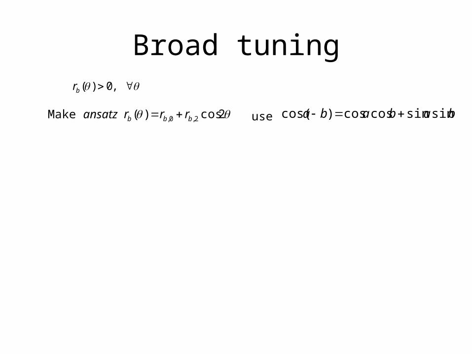
Broad tuning ,0)(br

Broad tuning ,0)(br
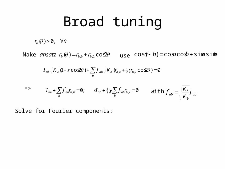
Make ansatz 2cos)( 2,0, bbb rrr
Broad tuning ,0)(br
Make ansatz 2cos)( 2,0, bbb rrr bababa sinsincoscos)cos( use

Broad tuning ,0)(br
Make ansatz 2cos)( 2,0, bbb rrr bababa sinsincoscos)cos( use
0)2cos()2cos1( 2,21
0,00 bbb
baba rrKJKI

Broad tuning ,0)(br
Make ansatz 2cos)( 2,0, bbb rrr bababa sinsincoscos)cos( use
0)2cos()2cos1( 2,21
0,00 bbb
baba rrKJKI
=> b
babab
baba rJIrJI 0ˆ;0ˆ2,2
100,0
abb
ab JKK
J0
ˆ with
Broad tuning ,0)(br
Make ansatz 2cos)( 2,0, bbb rrr bababa sinsincoscos)cos( use
0)2cos()2cos1( 2,21
0,00 bbb
baba rrKJKI
=> b
babab
baba rJIrJI 0ˆ;0ˆ2,2
100,0
abb
ab JKK
J0
ˆ with
Solve for Fourier components:

Broad tuning ,0)(br
Make ansatz 2cos)( 2,0, bbb rrr bababa sinsincoscos)cos( use
0)2cos()2cos1( 2,21
0,00 bbb
baba rrKJKI
=> b
babab
baba rJIrJI 0ˆ;0ˆ2,2
100,0
abb
ab JKK
J0
ˆ with
Solve for Fourier components:
20
10
2,2
2,1
20
10
0,2
0,1 ˆ2;ˆ
I
I
r
r
I
I
r
r1-1- JJ

Broad tuning ,0)(br
Make ansatz 2cos)( 2,0, bbb rrr bababa sinsincoscos)cos( use
0)2cos()2cos1( 2,21
0,00 bbb
baba rrKJKI
=> b
babab
baba rJIrJI 0ˆ;0ˆ2,2
100,0
abb
ab JKK
J0
ˆ with
Solve for Fourier components:
20
10
2,2
2,1
20
10
0,2
0,1 ˆ2;ˆ
I
I
r
r
I
I
r
r1-1- JJ
Valid for 21 (otherwise ra() < 0 at large )

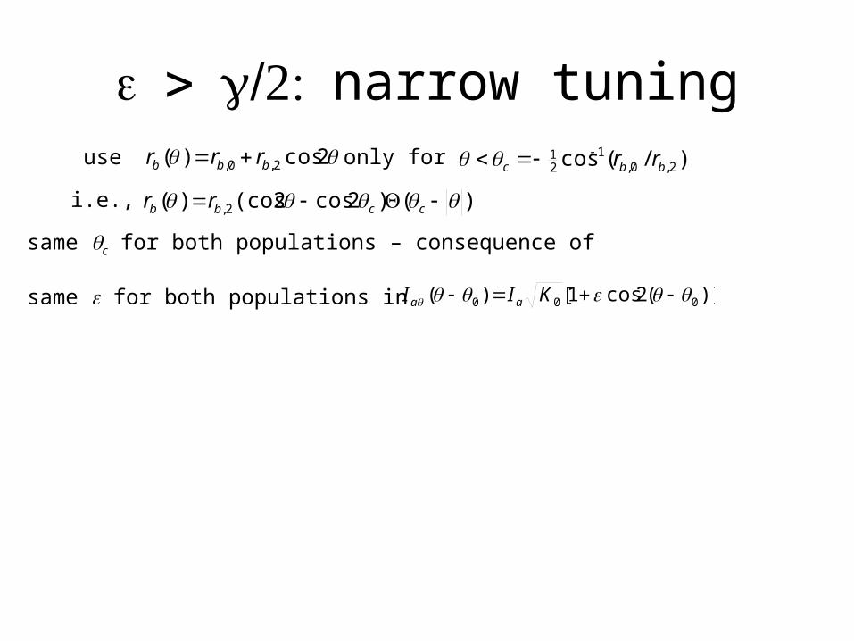
narrow tuning 2cos)( 2,0, bbb rrr use only for )/(cos 2,0,
121
bbc rr

narrow tuning 2cos)( 2,0, bbb rrr use only for )/(cos 2,0,
121
bbc rr
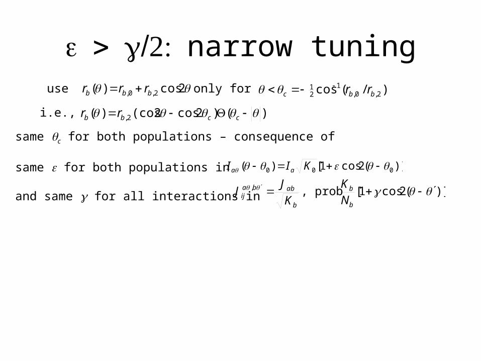
i.e., )()2cos2(cos)( 2, ccbb rr

narrow tuning 2cos)( 2,0, bbb rrr use only for )/(cos 2,0,
121
bbc rr
i.e., )()2cos2(cos)( 2, ccbb rr
same c for both populations – consequence of
narrow tuning 2cos)( 2,0, bbb rrr use only for )/(cos 2,0,
121
bbc rr
i.e., )()2cos2(cos)( 2, ccbb rr
same c for both populations – consequence of
same for both populations in )](2cos1[)( 000 KII aa
narrow tuning 2cos)( 2,0, bbb rrr use only for )/(cos 2,0,
121
bbc rr
i.e., )()2cos2(cos)( 2, ccbb rr
same c for both populations – consequence of
same for both populations in
and same for all interactions in
)](2cos1[)( 000 KII aa
)](2cos1[prob,,
b
b
b
abbaij N
K
K
JJ

narrow tuning 2cos)( 2,0, bbb rrr use only for )/(cos 2,0,
121
bbc rr
i.e., )()2cos2(cos)( 2, ccbb rr
same c for both populations – consequence of
same for both populations in
and same for all interactions in
)](2cos1[)( 000 KII aa
)](2cos1[prob,,
b
b
b
abbaij N
K
K
JJ
0)()](2cos1[)2cos1(2/
2/00
b
bbaba r
dKJKI
Balance condition:

narrow tuning 2cos)( 2,0, bbb rrr use only for )/(cos 2,0,
121
bbc rr
i.e., )()2cos2(cos)( 2, ccbb rr
same c for both populations – consequence of
same for both populations in
and same for all interactions in
)](2cos1[)( 000 KII aa
)](2cos1[prob,,
b
b
b
abbaij N
K
K
JJ
0)2cos2(cos)2cos2cos1(
)2cos1(
2,
00
cbb
bab
a
rd
KJ
KI
c
c
0)()](2cos1[)2cos1(2/
2/00
b
bbaba r
dKJKI
Balance condition:
=>
Narrow tuning (2)
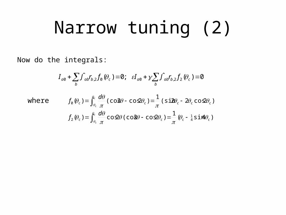
Now do the integrals:

Narrow tuning (2)
Now do the integrals:
0)(ˆ;0)(ˆ22,002,0
bcbaba
bcbaba frJIfrJI
Narrow tuning (2)
Now do the integrals:
0)(ˆ;0)(ˆ22,002,0
bcbaba
bcbaba frJIfrJI
)4sin(1
)2cos2(cos2cos)(
)2cos22(sin1
)2cos2(cos)(
41
2
0
cccc
ccccc
c
c
c
c
df
df
where

Narrow tuning (2)
Now do the integrals:
0)(ˆ;0)(ˆ22,002,0
bcbaba
bcbaba frJIfrJI
)4sin(1
)2cos2(cos2cos)(
)2cos22(sin1
)2cos2(cos)(
41
2
0
cccc
ccccc
c
c
c
c
df
df
where
f0:f2:
______
----------
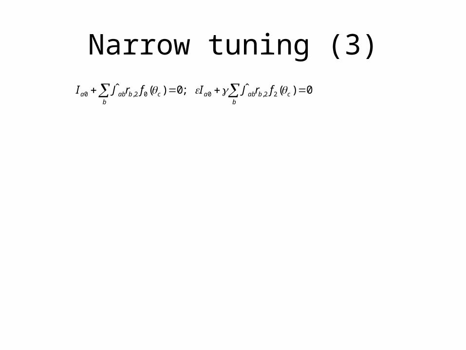
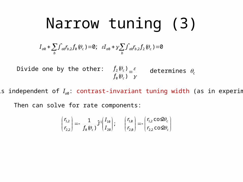
Narrow tuning (3)0)(ˆ;0)(ˆ
22,002,0 b
cbabab
cbaba frJIfrJI

Narrow tuning (3)0)(ˆ;0)(ˆ
22,002,0 b
cbabab
cbaba frJIfrJI
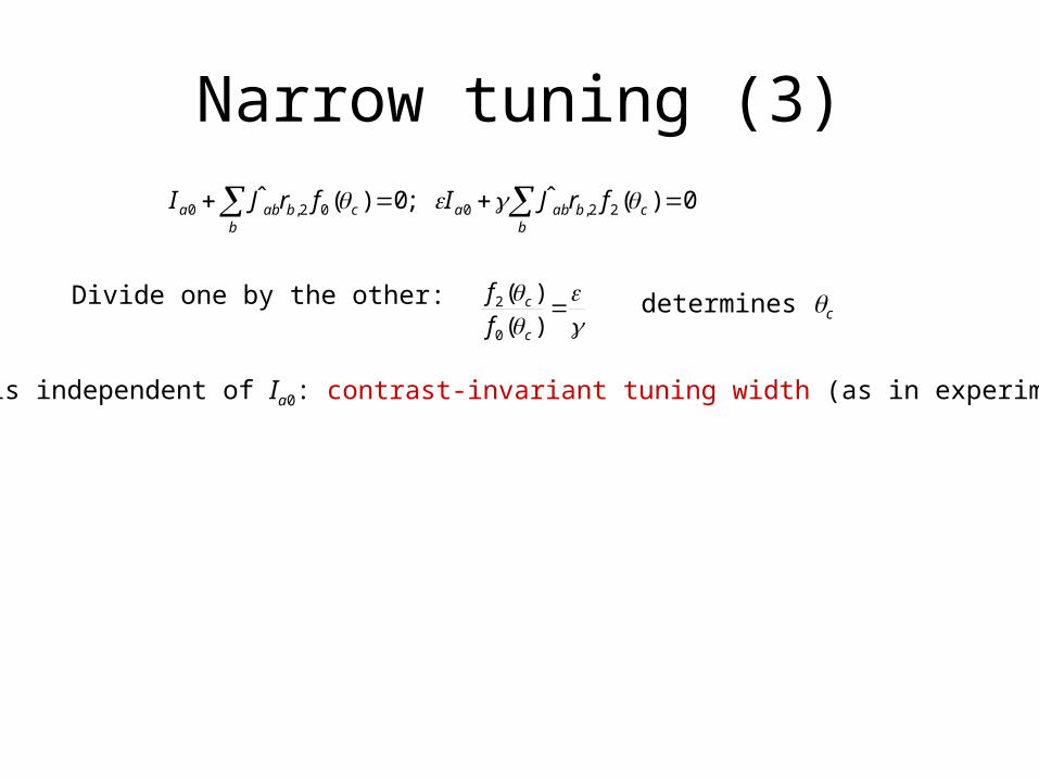
Divide one by the other:

Narrow tuning (3)0)(ˆ;0)(ˆ
22,002,0 b
cbabab
cbaba frJIfrJI
Divide one by the other:
)(
)(
0
2
c
c
f
f determines c
Narrow tuning (3)0)(ˆ;0)(ˆ
22,002,0 b
cbabab
cbaba frJIfrJI
Divide one by the other:
)(
)(
0
2
c
c
f
f determines c
c is independent of Ia0: contrast-invariant tuning width (as in experiments)

Narrow tuning (3)0)(ˆ;0)(ˆ
22,002,0 b
cbabab
cbaba frJIfrJI
Divide one by the other:
)(
)(
0
2
c
c
f
f determines c
c is independent of Ia0: contrast-invariant tuning width (as in experiments)
Then can solve for rate components:
Narrow tuning (3)0)(ˆ;0)(ˆ
22,002,0 b
cbabab
cbaba frJIfrJI
Divide one by the other:
)(
)(
0
2
c
c
f
f determines c
c is independent of Ia0: contrast-invariant tuning width (as in experiments)
Then can solve for rate components:
c
c-
c r
r
r
r
I
I
fr
r
2cos
2cos;ˆ
)(1
2,2
2,1
0,2
0,1
20
101
02,2
2,1J
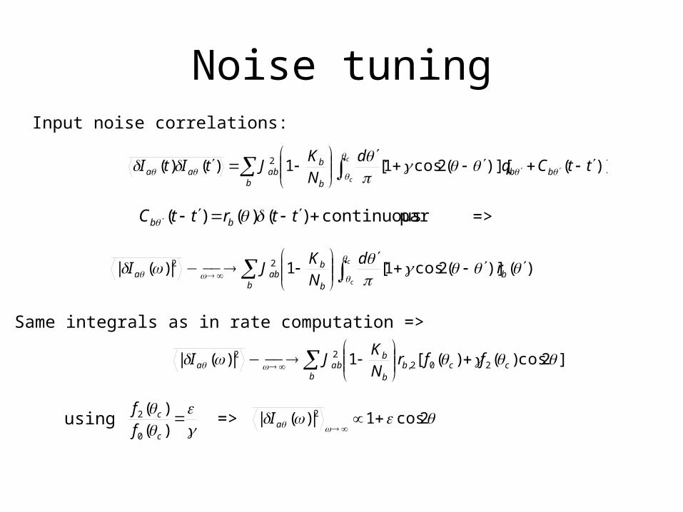
Noise tuningInput noise correlations:

Noise tuning
)]()][(2cos1[1)()( 2 ttCqd
NK
JtItI bbb
b
babaa
c
c
Input noise correlations:

Noise tuning
)]()][(2cos1[1)()( 2 ttCqd
NK
JtItI bbb
b
babaa
c
c
Input noise correlations:
partcontinuous)()()( ttrttC bb

Noise tuning
)]()][(2cos1[1)()( 2 ttCqd
NK
JtItI bbb
b
babaa
c
c
Input noise correlations:
partcontinuous)()()( ttrttC bb =>
)()](2cos1[1|)(| 22
b
b
b
baba r
dNK
JIc
c

Noise tuning
)]()][(2cos1[1)()( 2 ttCqd
NK
JtItI bbb
b
babaa
c
c
Input noise correlations:
partcontinuous)()()( ttrttC bb =>
)()](2cos1[1|)(| 22
b
b
b
baba r
dNK
JIc
c
Same integrals as in rate computation =>

Noise tuning
)]()][(2cos1[1)()( 2 ttCqd
NK
JtItI bbb
b
babaa
c
c
Input noise correlations:
partcontinuous)()()( ttrttC bb =>
)()](2cos1[1|)(| 22
b
b
b
baba r
dNK
JIc
c
Same integrals as in rate computation =>
]2cos)()([1|)(| 202,22 ccb
b
b
baba ffr
NK
JI

Noise tuning
)]()][(2cos1[1)()( 2 ttCqd
NK
JtItI bbb
b
babaa
c
c
Input noise correlations:
partcontinuous)()()( ttrttC bb =>
)()](2cos1[1|)(| 22
b
b
b
baba r
dNK
JIc
c
Same integrals as in rate computation =>
)(
)(
0
2
c
c
f
fusing
]2cos)()([1|)(| 202,22 ccb
b
b
baba ffr
NK
JI
Noise tuning
)]()][(2cos1[1)()( 2 ttCqd
NK
JtItI bbb
b
babaa
c
c
Input noise correlations:
partcontinuous)()()( ttrttC bb =>
)()](2cos1[1|)(| 22
b
b
b
baba r
dNK
JIc
c
Same integrals as in rate computation =>
2cos1|)(| 2
aI
)(
)(
0
2
c
c
f
fusing =>
]2cos)()([1|)(| 202,22 ccb
b
b
baba ffr
NK
JI

Noise tuning
)]()][(2cos1[1)()( 2 ttCqd
NK
JtItI bbb
b
babaa
c
c
Input noise correlations:
partcontinuous)()()( ttrttC bb =>
)()](2cos1[1|)(| 22
b
b
b
baba r
dNK
JIc
c
Same integrals as in rate computation =>
2cos1|)(| 2
aI
)(
)(
0
2
c
c
f
fusing =>
]2cos)()([1|)(| 202,22 ccb
b
b
baba ffr
NK
JI
Same tuning as input!

Some numerical results (1)

Numerical results (2):Fano factor tuning

Numerical results (3): noise tuning vs firing tuning