lecture 12: analysis of nonlinear systems. phase...

ISS0031 Modeling and Identification

Lecture 12: Analysis of Nonlinear Systems. Phase

Plane analysis. Linearization.

Aleksei Tepljakov, Ph.D.

November 25, 2015

Recall: State Space Representation ofDynamic Systems

Aleksei Tepljakov 2 / 22

Suppose that a system has p inputs ui(t), i = 1, 2, . . . , p, and q outputs yk(t),k = 1, 2, . . . , q, and there are n system states that make up a state variable

vector x =[

x1 x2 · · · xn

]T

. The state space expression of generaldynamic systems can be written as

{

xi = fi(x1, x2, . . . , xn, u1, u2, . . . , up), i = 1, 2, . . . , n,

yk = gk(x1, x2, . . . , xn, u1, u2, . . . , up), k = 1, 2, . . . , q,(1)

where fi(·) and gk(·) can be any nonlinear functions. For linear, time-invariantsystems the state space expression is

{

x = Ax+Bu,

y = Cx+Du,(2)

where u =[

u1 u2 · · · un

]T

and y =[

y1 y2 · · · yq]T

are theinput and output vectors, respectively. The matrices A,B,C, and D arecompatible matrices with sizes n× n, n× p, q × n, and q × p, respectively.

Examples of Nonlinear Phenomena


• Finite escape time. The state of an unstable nonlinear system cango to infinity in finite time, whereas the state of an unstable linearsystem goest to infinity as time approaches infinity.

• Multiple isolated equilibrium points. A nonlinear system may havemore than one isolated equilibrium point. The state may converge toone of several steady-state operating points. A linear system, on theother hand, can have only one isolated equilibrium point. Therefore,it has a single steady-state operating point that attracts the state ofthe system without regard to the initial state.

• Limit cycles. A stable oscillation of fixed amplitude and frequencyirrespective on the initial state should be produced by a nonlinearsystem, since for a linear system to oscillate a nonrobust conditionmust be fulfilled—it will be very difficult to maintain stable oscillationin the presence of perturbations (e.g., disturbances).

Examples of Nonlinear Phenomena(continued)


• (Sub)harmonic or almost periodic oscillations. Under a periodicinput signal a nonlinear system may not produce an output of thesame frequency; moreover, it may produce an almost periodic signal.On the other hand, a stable linear system would produce an output ofthe same frequency.

• Chaos. A nonlinear system may have a complicated steady-statebehavior that is not equivilibrium, or (almost) periodic oscillation.The system may also exhibit random behavior.

• Multiple modes of behavior. A nonlinear system may exhibit twoor more modes of behavior. For example, an unforced system mayhave more than one limit cycle. A forced system with periodicexcitation may exhibit (sub)harmonic or a more complicatedsteady-state behavior, depending on the amplitude and frequency ofthe input. It may even exhibit a discontinuous jump in the mode ofbehavior as the input excitation is smoothly changed.

Example: Pendulum Equation


l

mg

θ

The law of motion is described by

mlθ = −mg sin θ − klθ, (3)

where m is the mass of the payload, l is the length of therod, g is gravitational acceleration, and k is a frictioncoefficient.Take x1 = θ and x2 = θ.The state model isobtained as

x1 = x2 (4)

x2 = −g

lsinx1 −

k

mx2. (5)

Solving for zero dynamics yields equilibrium points that

are located at x0n = (nπ, 0), for n = 0,±1,±2, . . . .

Modeling Dynamic Systems: Dealing withInput and Output Nonlinearities


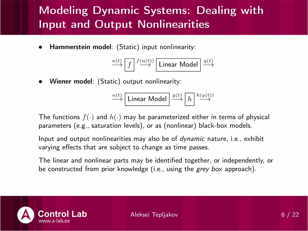
• Hammerstein model: (Static) input nonlinearity:

u(t)−→ f

f(u(t))−→ Linear Model

y(t)−→

• Wiener model: (Static) output nonlinearity:

u(t)−→ Linear Model

y(t)−→ h

h(y(t))−→

The functions f(·) and h(·) may be parameterized either in terms of physicalparameters (e.g., saturation levels), or as (nonlinear) black-box models.

Input and output nonlinearities may also be of dynamic nature, i.e., exhibitvarying effects that are subject to change as time passes.

The linear and nonlinear parts may be identified together, or independently, orbe constructed from prior knowledge (i.e., using the grey box approach).

Common Nonlinearities: Ideal Saturation


y

u

k

δ

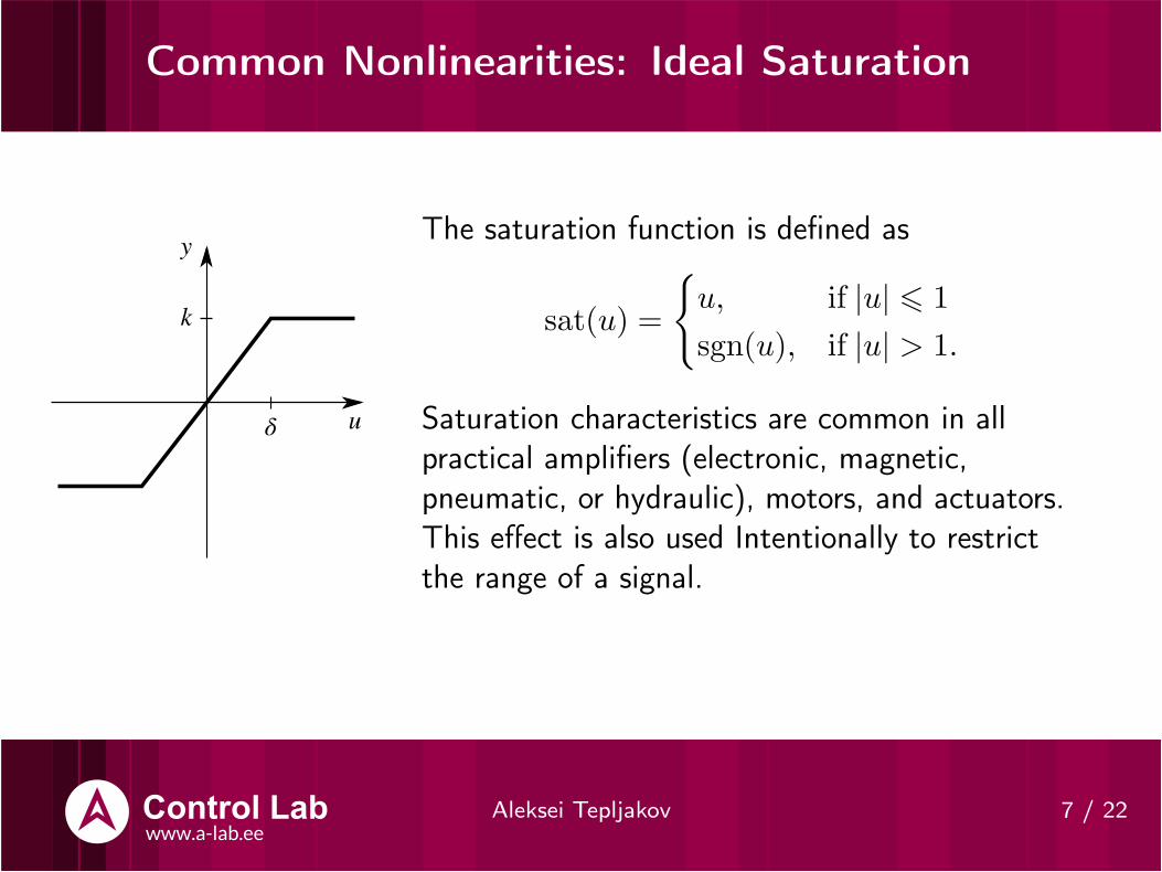
The saturation function is defined as

sat(u) =

{

u, if |u| 6 1

sgn(u), if |u| > 1.

Saturation characteristics are common in allpractical amplifiers (electronic, magnetic,pneumatic, or hydraulic), motors, and actuators.This effect is also used Intentionally to restrictthe range of a signal.

Common Nonlinearities: Ideal Relay


y

u

1

-1

An ideal relay may be described by the signumfunction as

sgn(u) =

1, if u > 0

0, if u = 0

−1, if u < 0.

This nonlinear characteristic can modelelectromechanical relays, thyristor circuits, andother switching devices. The relay characteristicis also used in various control applications (e.g.,heating), where it is usual to consider hysteresis.

Common Nonlinearities: Ideal Dead Zone


y

uδ

The dead-zone (also called deadband)characteristic may be defined by a function

d(u) =

{

0, if |u| 6 δ

u, if |u| > δ.

This characteristic is typical of valves and someamplifiers at low input signals. The backlash

effect known from gear interactions in amechanical system may be approximated by thedead-zone effect.

Common Nonlinearities: Ideal Quantization


y

uq

2

q

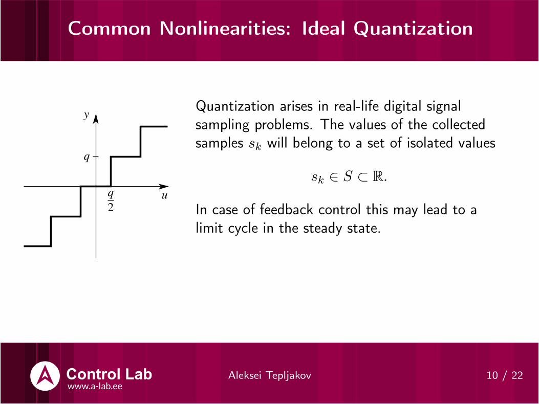
Quantization arises in real-life digital signalsampling problems. The values of the collectedsamples sk will belong to a set of isolated values

sk ∈ S ⊂ R.

In case of feedback control this may lead to alimit cycle in the steady state.

Common Nonlinearities: Hysteresis


y

u

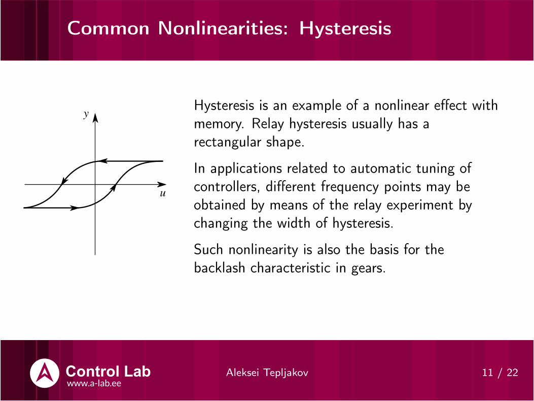
Hysteresis is an example of a nonlinear effect withmemory. Relay hysteresis usually has arectangular shape.

In applications related to automatic tuning ofcontrollers, different frequency points may beobtained by means of the relay experiment bychanging the width of hysteresis.

Such nonlinearity is also the basis for thebacklash characteristic in gears.

Second-order Systems: Essential Definitions


A second-order autonomous system is represented by two scalardifferential equations

{

x1 = f1(x1, x2)

x2 = f2(x1, x2).(6)

Let x(t) = (x1(t), x2(t)) be the solution of (6) that starts at a certaininitial state x0 = (x10, x20). The locus in the (x1-x2)-plane of thesolution x(t) for all t > 0 is a curve that passes through the point x0.This curve is called a trajectory or orbit of (6) from x0. The(x1-x2)-plane is called state plane or phase plane. Using vector notation

x = f(x), (7)

where f(x) = (f1(x), f2(x)) we consider f(x) as a vector field on thestate plane. The family of all trajectories is called the phase portrait ofthe system (6).

Qualitative Behavior of Linear Systems


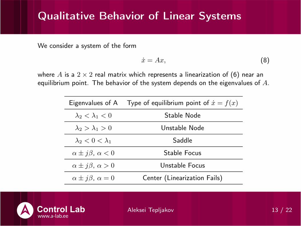
We consider a system of the form

x = Ax, (8)

where A is a 2× 2 real matrix which represents a linearization of (6) near anequilibrium point. The behavior of the system depends on the eigenvalues of A.

Eigenvalues of A Type of equilibrium point of x = f(x)

λ2 < λ1 < 0 Stable Node

λ2 > λ1 > 0 Unstable Node

λ2 < 0 < λ1 Saddle

α± jβ, α < 0 Stable Focus

α± jβ, α > 0 Unstable Focus

α± jβ, α = 0 Center (Linearization Fails)

Qualitative Behavior of Linear Systems(continued)


x2

x1

x2

x1

x2

x1

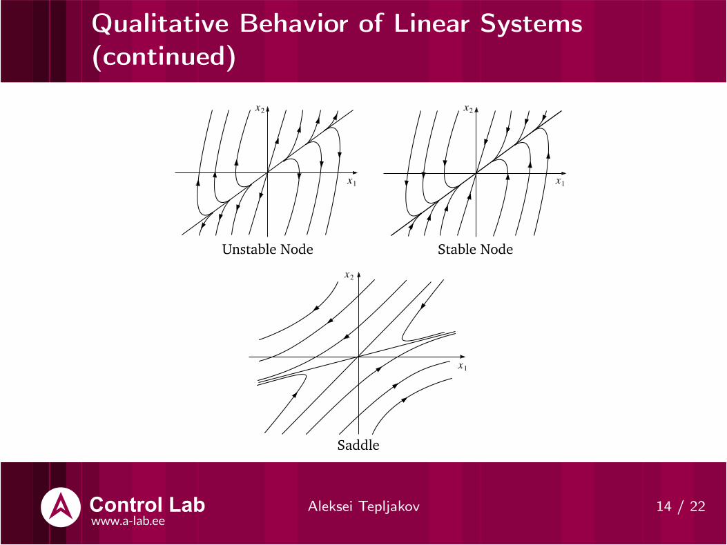
Unstable Node Stable Node

Saddle

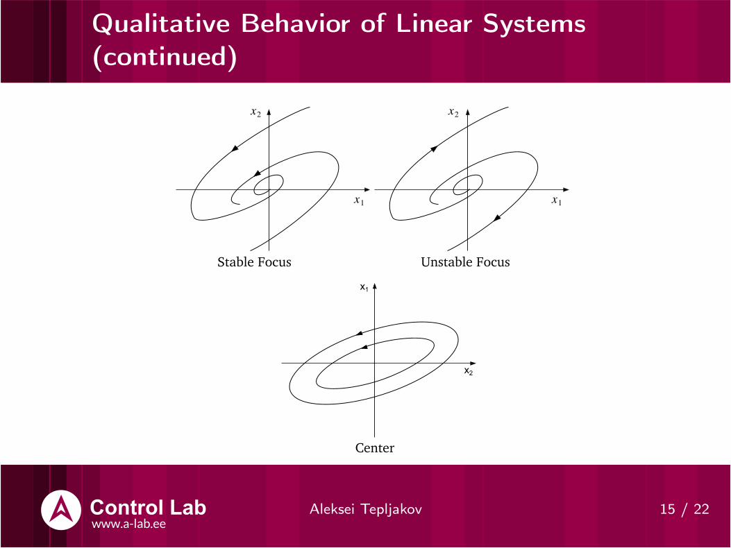
Qualitative Behavior of Linear Systems(continued)


x1

x2

x1

x2

x1

x2

Stable Focus Unstable Focus

Center

Limit Cycles


x1

x2

Stable Limit Cycle Unstable Limit Cycle

x1

x2

An isolated periodic orbit is called a limit cycle. The limit cycle is stable

if all trajectories in the vicinity of the limit cycle ultimately tend toward

the limit cycle, and unstable if all trajectories starting from points

arbitrarily close to the limit cycle will tend away from it, as t → ∞.

Nonlinear Systems: Definition of Stability


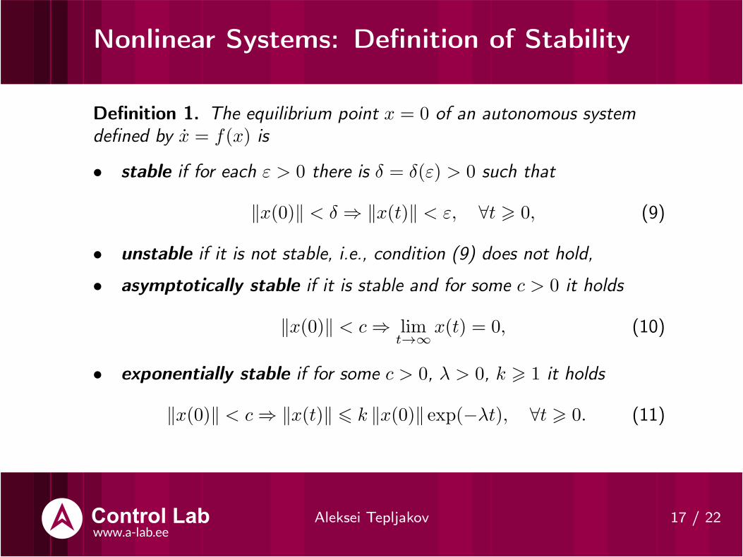
Definition 1. The equilibrium point x = 0 of an autonomous systemdefined by x = f(x) is

• stable if for each ε > 0 there is δ = δ(ε) > 0 such that

‖x(0)‖ < δ ⇒ ‖x(t)‖ < ε, ∀t > 0, (9)

• unstable if it is not stable, i.e., condition (9) does not hold,

• asymptotically stable if it is stable and for some c > 0 it holds

‖x(0)‖ < c ⇒ limt→∞

x(t) = 0, (10)

• exponentially stable if for some c > 0, λ > 0, k > 1 it holds

‖x(0)‖ < c ⇒ ‖x(t)‖ 6 k ‖x(0)‖ exp(−λt), ∀t > 0. (11)

Linearization: Data Fitting (Identification)


As a nonlinear system may have several operating points, the approach tolinearization may be the following:

1. Choose a set of n operating points of the form (uk, yk), k = 1, 2, . . . , n.The number of operating points depends on the dynamic range of thesystem output and/or the control problem.

2. Obtain a linear model in the vicinity of each of the operating points, e.g.:

(a) Perform a step experiment and use time-domain identification;

(b) Use the relay feedback method to collect frequency response pointsand use frequency-domain identification.

3. Design a switching law for the set of linear systems to form the completenonlinear model and validate it.

4. If only control is desired, design a (linear) controller for each operatingpoint and design a control switching law.

Feedback Linearization: Motivation:Pendulum Example


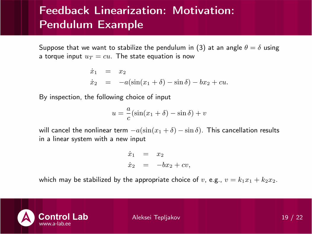
Suppose that we want to stabilize the pendulum in (3) at an angle θ = δ usinga torque input uT = cu. The state equation is now

x1 = x2

x2 = −a(sin(x1 + δ)− sin δ)− bx2 + cu.

By inspection, the following choice of input

u =a

c(sin(x1 + δ)− sin δ) + v

will cancel the nonlinear term −a(sin(x1 + δ)− sin δ). This cancellation resultsin a linear system with a new input

x1 = x2

x2 = −bx2 + cv,

which may be stabilized by the appropriate choice of v, e.g., v = k1x1 + k2x2.

Feedback Linearization: General Result


Definition 2. A nonlinear system

y = f(y) +G(y)u, (12)

where f : U → Rn and G : U → R

n×p are sufficiently smooth on a

domain U ⊂ Rn, is said to be feedback linearizable if there exists

a diffeomorphism T : U → Rn such that D = T (U) contains the

origin and the change of variables x = T (y) transforms the

system (12) into the form

x = Ax+Bβ−1(x)(u− α(x)) (13)

with (A,B) controllable and β(x) nonsingular for all x ∈ D.

Where To Go From Here: Approaches toNonlinear System Analysis


1. Differential Geometry:

• Application of differential and integral calculus to the study ofproblems in geometry.

• Reference: H. Khalil, Nonlinear Systems, 3rd ed., Prentice Hall, UpperSaddle River, NJ, 2002.

2. Differential Algebra:

• Study of various algebraic objects (differential rings, fields, andalgebras) and their application to the study of differential equations.

• Reference: G. Conte, C.H. Moog, A.M. Perdon, Algebraic Methods for

Nonlinear Control Systems: Theory and Applications, 2nd ed.,Springer-Verlag, London, 2007.

Questions?


Thank you for your attention!

NB! Next time we do Test #2.

lecture 12: analysis of nonlinear systems. phase...

Documents