lecture 12: parallel sorting - uic engineering · lecture 12: parallel sorting shantanu dutt ece...
TRANSCRIPT

Lecture 12: Parallel Sorting
Shantanu Dutt
ECE Dept.
UIC

Acknowledgement
• Adapted from Chapter 9 slides of the text, by A. Grama w/ a few changes, augmentations and corrections made by Shantanu Dutt in colored text.
Topic Overview
• Issues in Sorting on Parallel Computers
• Bitonic Sorting Networks
• Bitonic Sorting on Hypercubes and 2-D Meshes

Sorting: Overview
• One of the most commonly used and well-studied kernels.
• Sorting can be comparison-based or non-comparison-based.
• The fundamental operation of comparison-based sorting is compare-exchange.
• The lower bound on any comparison-based sort of n numbers is Θ(nlog n) .
• We focus here on comparison-based sorting algorithms.

Sorting: Basics
What is a parallel sorted sequence? Where are the input and output lists stored?
• We assume that the input and output lists are distributed.
• The sorted list is partitioned with the property that each partitioned list is sorted and each element in processor Pi's list is less than or equal to that in Pj's list if i < j.

Sorting: Parallel Compare Exchange
Operation
A parallel compare-exchange operation. Processes Pi
and Pj send their elements to each other. Process Pi keeps min{ai,aj}, and Pj keeps max{ai, aj}.
Sorting: Basics What is the parallel counterpart to a sequential comparator?
• If each processor has one element, the compare exchange operation stores the smaller element at the processor with smaller id. This can be done in ts + tw time.
• If we have more than one element per processor, we call this operation a compare split. Assume each of two processors have n/p elements.
• After the compare-split operation, the smaller n/p elements are at processor Pi and the larger n/p elements at Pj, where i < j.
• The commun. time for a compare-split operation is (ts+ twn/p), and assuming that the two partial lists were initially sorted, the computation time is Q(2n/p)—essentially, the time to merge two sorted lists.

Sorting: Parallel Compare Split Operation
A compare-split operation. Each process sends its block of size n/p to the other process. Each process merges the received
block with its own block and retains only the appropriate half of the merged block. In this example, process Pi retains the smaller elements and process Pi retains the larger elements.
Sorting Networks
• Networks of comparators designed specifically for sorting.
• A comparator is a device with two inputs x and y and two outputs x' and y'. For an increasing comparator, x' = min{x,y} and y' = max{x,y}; and vice-versa for a decreasing comparator.
• We denote an increasing comparator by and a decreasing comparator by Ө.
• The speed of the network is proportional to its depth.
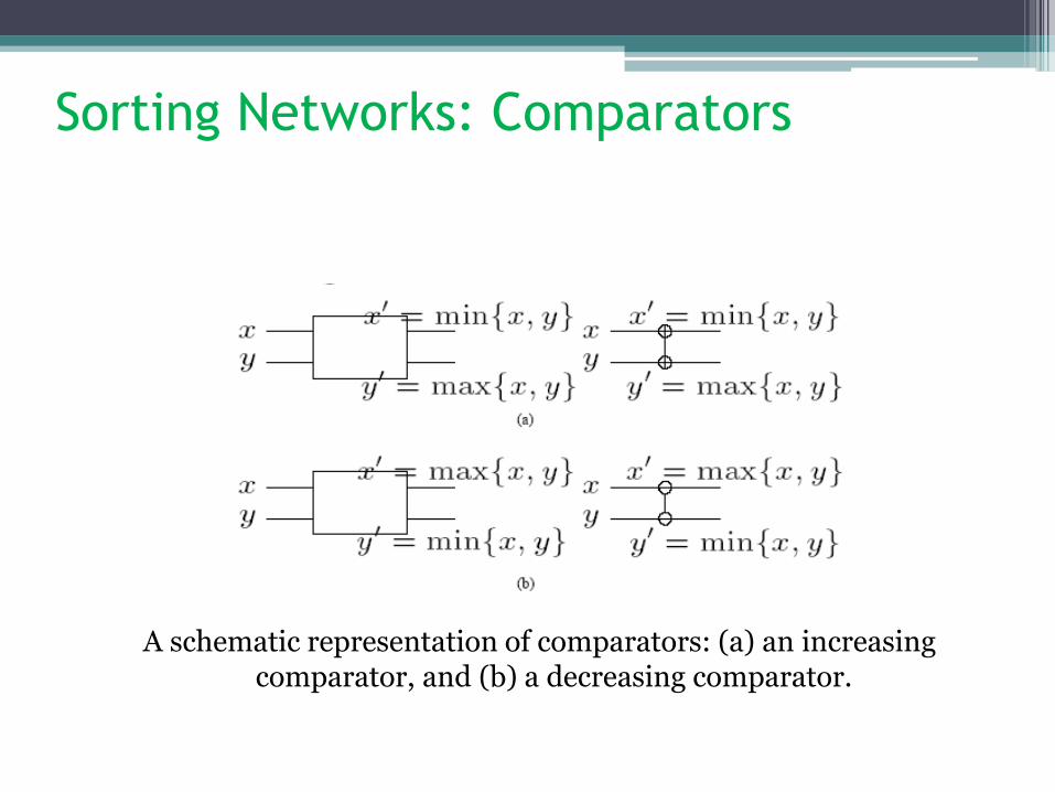
Sorting Networks: Comparators
A schematic representation of comparators: (a) an increasing comparator, and (b) a decreasing comparator.

Sorting Networks
A typical sorting network. Every sorting network is made up of a series of columns, and each column contains a number
of comparators connected in parallel.
Sorting Networks: Bitonic Sort
• A bitonic sorting network sorts n elements in Θ(log2n) time.
• A bitonic sequence has two tones - increasing and decreasing, or vice versa. Any cyclic rotation of such sequences is also considered bitonic.
• 1,2,4,7,6,0 is a bitonic sequence, because it first increases (1 to 7) and then decreases (7 to 0). 8,9,2,1,0,4 is another bitonic sequence, because it is a cyclic shift of 0,4,8,9,2,1.
• The kernel of the network is the rearrangement of a bitonic sequence into a sorted sequence.
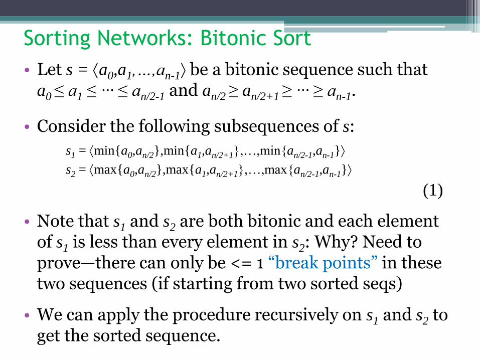
Sorting Networks: Bitonic Sort
• Let s = a0,a1,…,an-1 be a bitonic sequence such that a0 ≤ a1 ≤ ··· ≤ an/2-1 and an/2 ≥ an/2+1 ≥ ··· ≥ an-1.
• Consider the following subsequences of s:
s1 = min{a0,an/2},min{a1,an/2+1},…,min{an/2-1,an-1}
s2 = max{a0,an/2},max{a1,an/2+1},…,max{an/2-1,an-1}
(1)
• Note that s1 and s2 are both bitonic and each element of s1 is less than every element in s2: Why? Need to prove—there can only be <= 1 “break points” in these two sequences (if starting from two sorted seqs)
• We can apply the procedure recursively on s1 and s2 to get the sorted sequence.
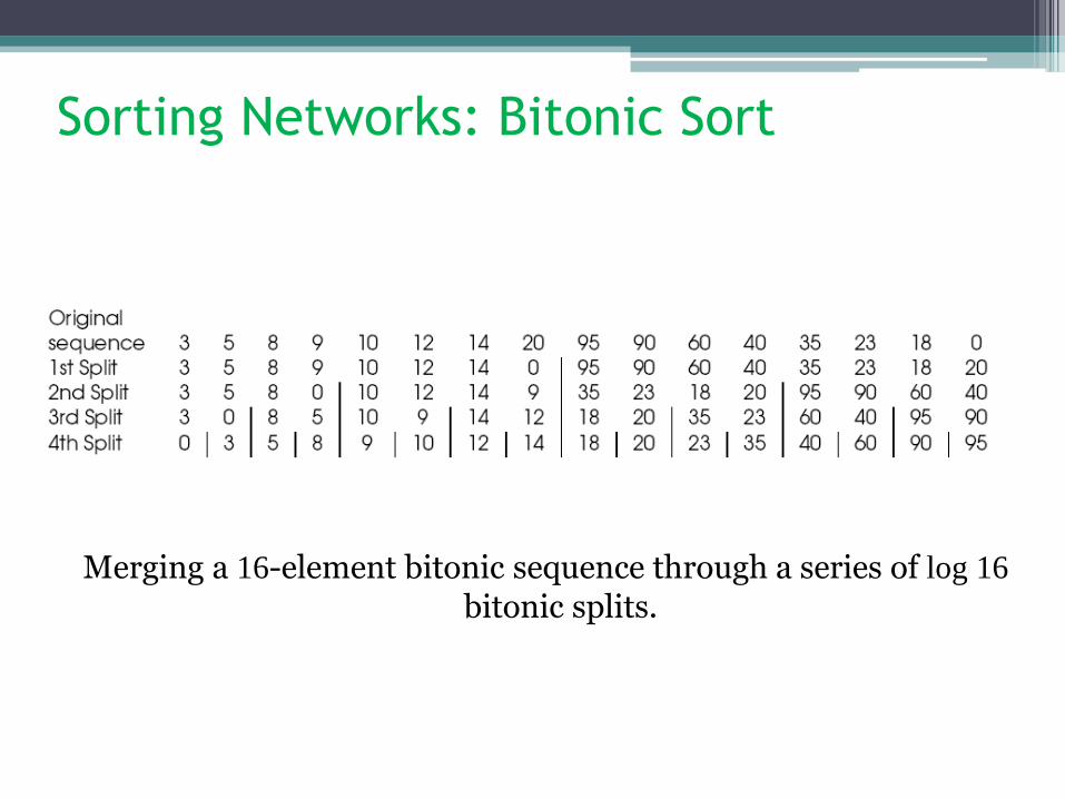
Sorting Networks: Bitonic Sort
Merging a 16-element bitonic sequence through a series of log 16 bitonic splits.

Sorting Networks: Bitonic Sort
• We can easily build a sorting network to implement this bitonic merge algorithm.
• Such a network is called a bitonic merging network.
• The network contains log n columns. Each column contains n/2 comparators and performs one step of the bitonic merge.
• We denote a bitonic merging network with n inputs by BM[n].
• Replacing the comparators by Ө comparators results in a decreasing output sequence; such a network is denoted by ӨBM[n].
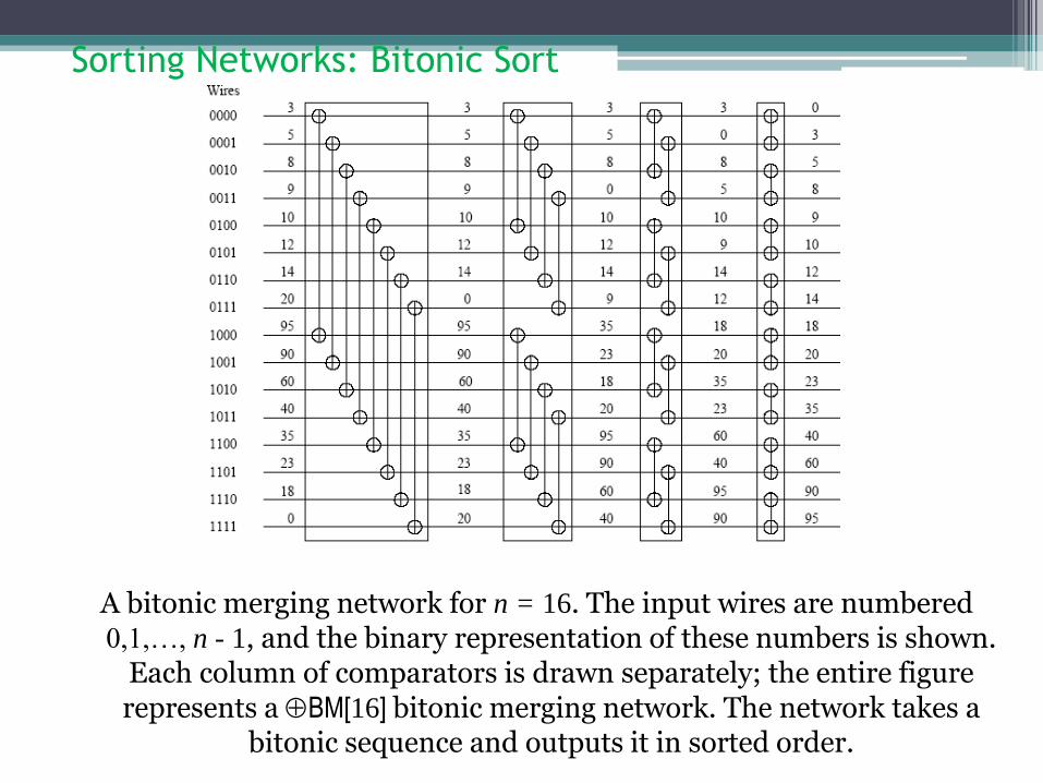
Sorting Networks: Bitonic Sort
A bitonic merging network for n = 16. The input wires are numbered 0,1,…, n - 1, and the binary representation of these numbers is shown.
Each column of comparators is drawn separately; the entire figure represents a BM[16] bitonic merging network. The network takes a
bitonic sequence and outputs it in sorted order.
Sorting Networks: Bitonic Sort
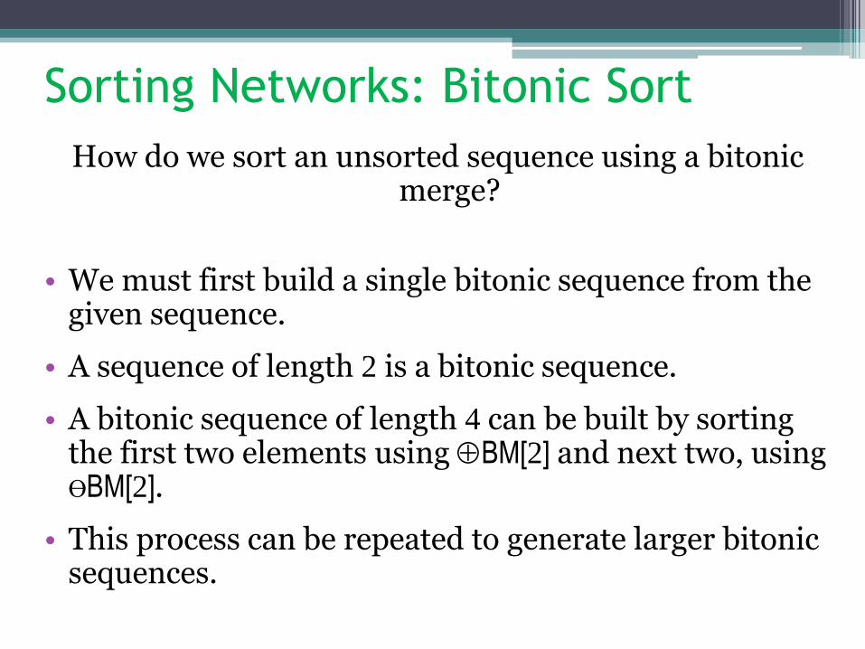
How do we sort an unsorted sequence using a bitonic merge?
• We must first build a single bitonic sequence from the given sequence.
• A sequence of length 2 is a bitonic sequence.
• A bitonic sequence of length 4 can be built by sorting the first two elements using BM[2] and next two, using ӨBM[2].
• This process can be repeated to generate larger bitonic sequences.

Sorting Networks: Bitonic Sort
A schematic representation of a network that converts an input
sequence into a bitonic sequence. In this example, BM[k] and
ӨBM[k] denote bitonic merging networks of input size k that
use and Ө comparators, respectively. The last merging
network (BM[16]) sorts the input. In this example, n = 16.

Sorting Networks: Bitonic Sort
The comparator network that transforms an input sequence of 16 unordered numbers into a bitonic sequence.

Sorting Networks: Bitonic Sort
• The depth of the network is Θ(log2 n).
• Each stage of the network contains n/2 comparators. A serial implementation of the network would have complexity Θ(nlog2 n).
Mapping Bitonic Sort to Hypercubes
• Consider the case of one item per processor. The question becomes one of how the wires in the bitonic network should be mapped to the hypercube interconnect.
• Note from our earlier examples that the compare-exchange operation is performed between two wires only if their labels differ in exactly one bit!
• This implies a direct mapping of wires to processors. All communication is nearest neighbor!
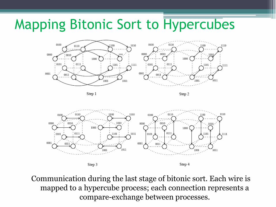
Mapping Bitonic Sort to Hypercubes
Communication during the last stage of bitonic sort. Each wire is mapped to a hypercube process; each connection represents a
compare-exchange between processes.

Mapping Bitonic Sort to Hypercubes
Communication characteristics of bitonic sort on a hypercube. During each stage of the algorithm, processes communicate along the
dimensions shown.

Mapping Bitonic Sort to Hypercubes
Parallel formulation of bitonic sort on a hypercube with n = 2d processes.
Augment d-bit labels to (d+1)-bit by concatenating a 0 at (d+1)-bit posn. of all d-bit labels;
/* The above condition stems from the more basic condition: if (i+1)’th bit is 0 (1) then need to perform increasing (decreasing) order sort, and thus if my j’th bit (current exchange dimension) is 1, I need to keep the max (min), and if 0, need to keep min (max) */
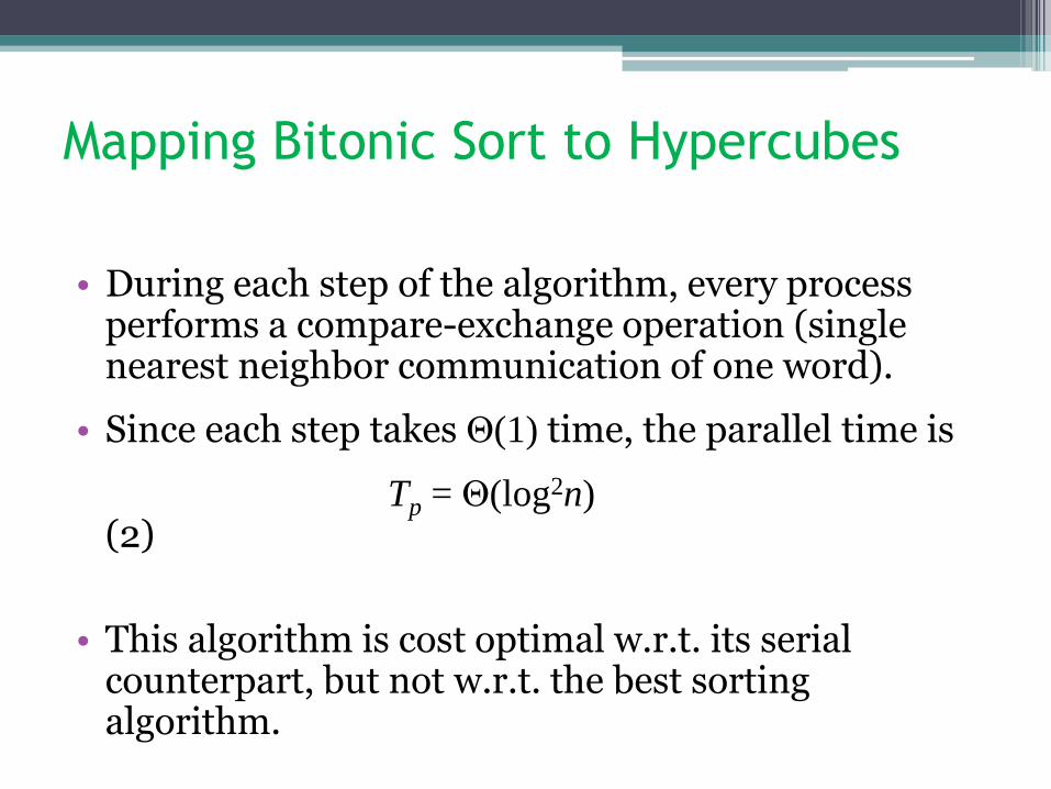
Mapping Bitonic Sort to Hypercubes
• During each step of the algorithm, every process performs a compare-exchange operation (single nearest neighbor communication of one word).
• Since each step takes Θ(1) time, the parallel time is
Tp = Θ(log2n) (2)
• This algorithm is cost optimal w.r.t. its serial counterpart, but not w.r.t. the best sorting algorithm.

Mapping Bitonic Sort to Meshes
• The connectivity of a mesh is lower than that of a hypercube, so we must expect some overhead in this mapping.
• Consider the row-major shuffled mapping of wires to processors.

Mapping Bitonic Sort to Meshes
Different ways of mapping the input wires of the bitonic sorting network to a mesh of processes: (a) row-major
mapping, (b) row-major snakelike mapping, and (c) row-major shuffled mapping.
Mapping Bitonic Sort to Meshes
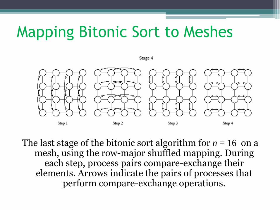
The last stage of the bitonic sort algorithm for n = 16 on a mesh, using the row-major shuffled mapping. During
each step, process pairs compare-exchange their elements. Arrows indicate the pairs of processes that
perform compare-exchange operations.

Mapping Bitonic Sort to Meshes
• In the row-major shuffled mapping, wires that differ at the ith least-significant bit are mapped onto mesh processes that are 2(i-1)/2 communication links away.
• The total amount of communication performed by each process is
• The total computation performed by each process is Θ(log2n).
• The parallel runtime is:
• Note that in the above analysis, conflict of msgs travelling 2k hops along a row an column not accounted for here—this sequentializes the commun. among 2k processors, resulting in a time of Q(22k), and ultimately total commun. time being Q(n) instead of Q(sqrt(n)).
• This is not cost optimal.
)(or ,72log
1 1
2/)1(nn
n
i
i
j
jQ

Block of Elements Per Processor
• Each process is assigned a block of n/p elements.
• The first step is a local sort of the local block.
• Each subsequent compare-exchange operation is replaced by a compare-split operation.
• We can effectively view the bitonic network as having (1 + log p)(log p)/2 steps.

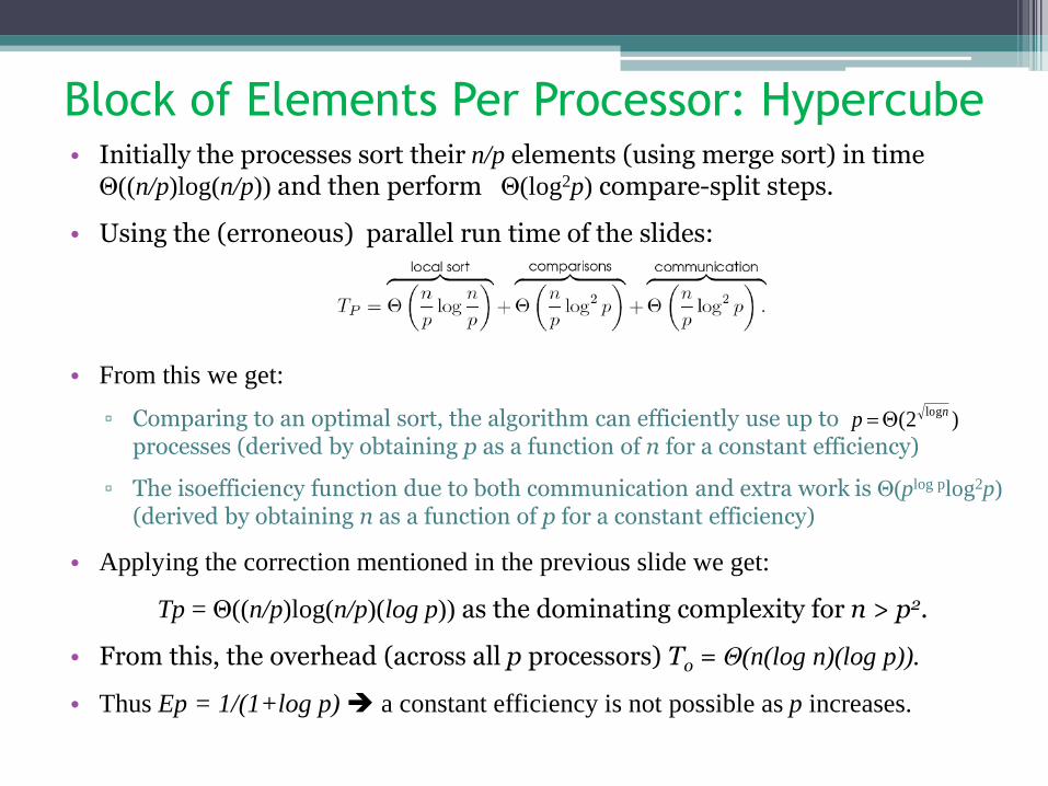
Block of Elements Per Processor: Hypercube • Initially the processes sort their n/p elements (using merge sort) in time
Θ((n/p)log(n/p)) and then perform Θ(log2p) compare-split steps.
• The parallel run time of this formulation is:
• The above expression seems to be not accounting for the internal sorting of a bitonic sequence of n/p numbers in each processor that is obtained after each stage of sorting 2i(n/p) numbers (in increasing or decreasing sequence in an i-dim. hypercube)—there are logP such stages, and after the (ith or last iteration of bitonic comparison-exchange for stage i sorting, each processor will have a bitonic sequence of n/p numbers that needs to be completely sorted (increasing or decreasing, depending on what the corresponding i-dim. hypercube is sorting—increasing if its (i+)’th dim. label is 0, else decreasing). This internal sorting can be done in Θ((n/p)log(n/p)) time using merge-sort (using an internal bitonic sort will take Θ((n/p)log2(n/p)) time). So the extra computation time (not accounted above) needed over log p stages is Θ((n/p)log(n/p)(log p)), and is the dominating complexity for n > p2.
• Comparing to an optimal sort, the algorithm can efficiently use up to processes (derived by obtaining p as a function of n for a constant efficiency)
• The isoefficiency function due to both communication and extra work is Θ(plog plog2p) (derived by obtaining n as a function of p for a constant efficiency)
)2(logn
p Q
Block of Elements Per Processor: Hypercube • Initially the processes sort their n/p elements (using merge sort) in time
Θ((n/p)log(n/p)) and then perform Θ(log2p) compare-split steps.
• Using the (erroneous) parallel run time of the slides:
• From this we get:
▫ Comparing to an optimal sort, the algorithm can efficiently use up to
processes (derived by obtaining p as a function of n for a constant efficiency)
▫ The isoefficiency function due to both communication and extra work is Θ(plog plog2p) (derived by obtaining n as a function of p for a constant efficiency)
• Applying the correction mentioned in the previous slide we get:
Tp = Θ((n/p)log(n/p)(log p)) as the dominating complexity for n > p2.
• From this, the overhead (across all p processors) To = Θ(n(log n)(log p)).
• Thus Ep = 1/(1+log p) a constant efficiency is not possible as p increases.
)2(logn
p Q
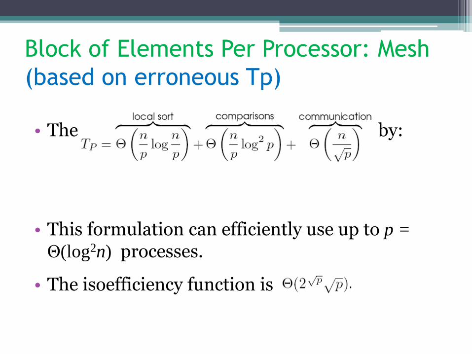
Block of Elements Per Processor: Mesh
(based on erroneous Tp)
• The parallel runtime in this case is given by:
• This formulation can efficiently use up to p =
Θ(log2n) processes.
• The isoefficiency function is
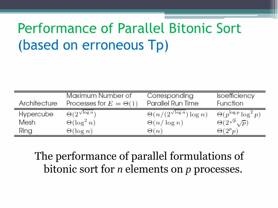
Performance of Parallel Bitonic Sort
(based on erroneous Tp)
The performance of parallel formulations of bitonic sort for n elements on p processes.