lecture 13 path modeling epsy 640 texas a&m university
Post on 22-Dec-2015
215 views
TRANSCRIPT

LECTURE 13PATH MODELING
EPSY 640
Texas A&M University

Path Modeling
• Effects:– Direct effect– Indirect effect
– Spurious effect
– Unanalyzed effect
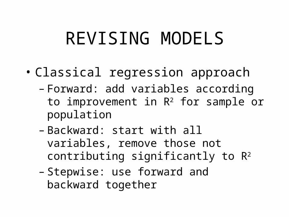
REVISING MODELS
• Classical regression approach– Forward: add variables according to
improvement in R2 for sample or population – Backward: start with all variables, remove
those not contributing significantly to R2
– Stepwise: use forward and backward together

REVISING MODELS
• SEM approach
• Model testing– improvement in fitting data
• Chi square test for model improvement (reduce model chi square significantly)
• Goodness of fit indices (based on chi square)– GFI, AGFI (proportional reduction in chi square)
– NFI, CFI (model improvement, adjusted for df)

REVISING MODELS
• Changing paths in classical or SEM regression and path analysis– t-test for significance of regression coefficient
(path coefficient)- test in unstandardized form– Lagrange Multiplier chi-square test that
restricted path should not be zero– Wald chi square test that free path should be
zero

REVISING MODELS
• t-test for significance of regression coefficient (path coefficient)- test in unstandardized form– coefficients are notoriously unstable in sample
estimation– worse in forward or backward selections– different issue for sample-to-sample variation
vs. sample-to-population variation
REVISING MODELS
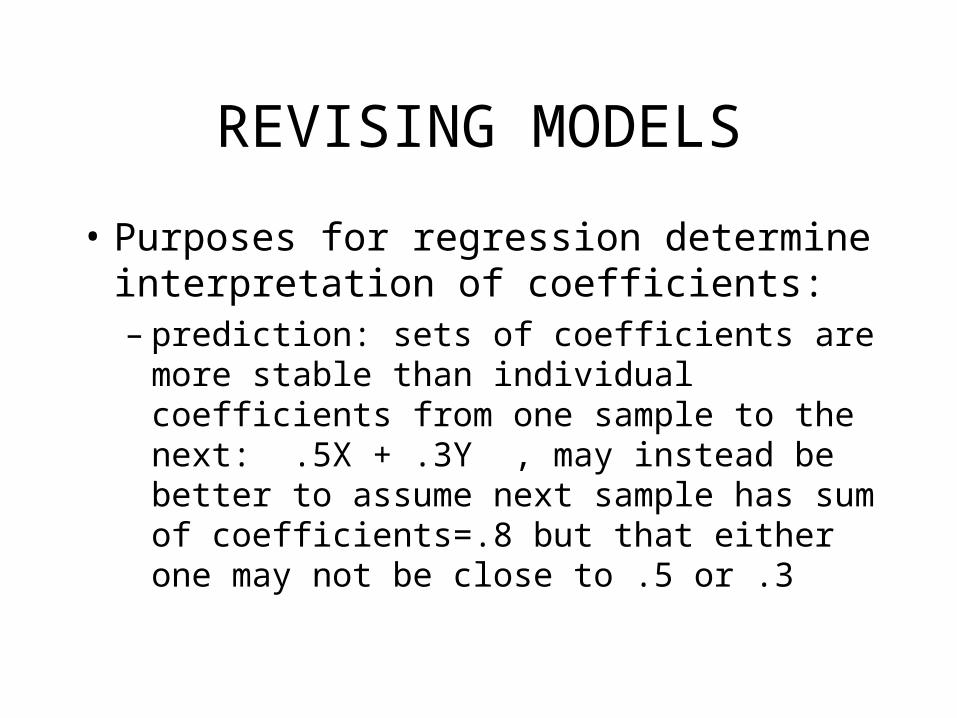
• Purposes for regression determine interpretation of coefficients:– prediction: sets of coefficients are more stable
than individual coefficients from one sample to the next: .5X + .3Y , may instead be better to assume next sample has sum of coefficients=.8 but that either one may not be close to .5 or .3

REVISING MODELS• Purposes for regression determine
interpretation of coefficients:– Theory-building: review of studies may provide
distribution of coefficients (effect sizes), try to fit current research finding into the distribution
– eg. Range of correlations between SES and IQ may be between -.1 and .6, mean of .33, SD=.15
– Did current result fit in the distribution?

REVISING MODELS• OUTLIER ANALYSIS
– Look at difference between predicted and actual score for each scores
– Which differences are large?– Which of the predictor scores are most
“discrepant” and causing the large difference in outcome?
– Remove outlier and rerun analysis; does it change meaning or coefficients?
– SPSS has such an analysis – VIF and CI indices
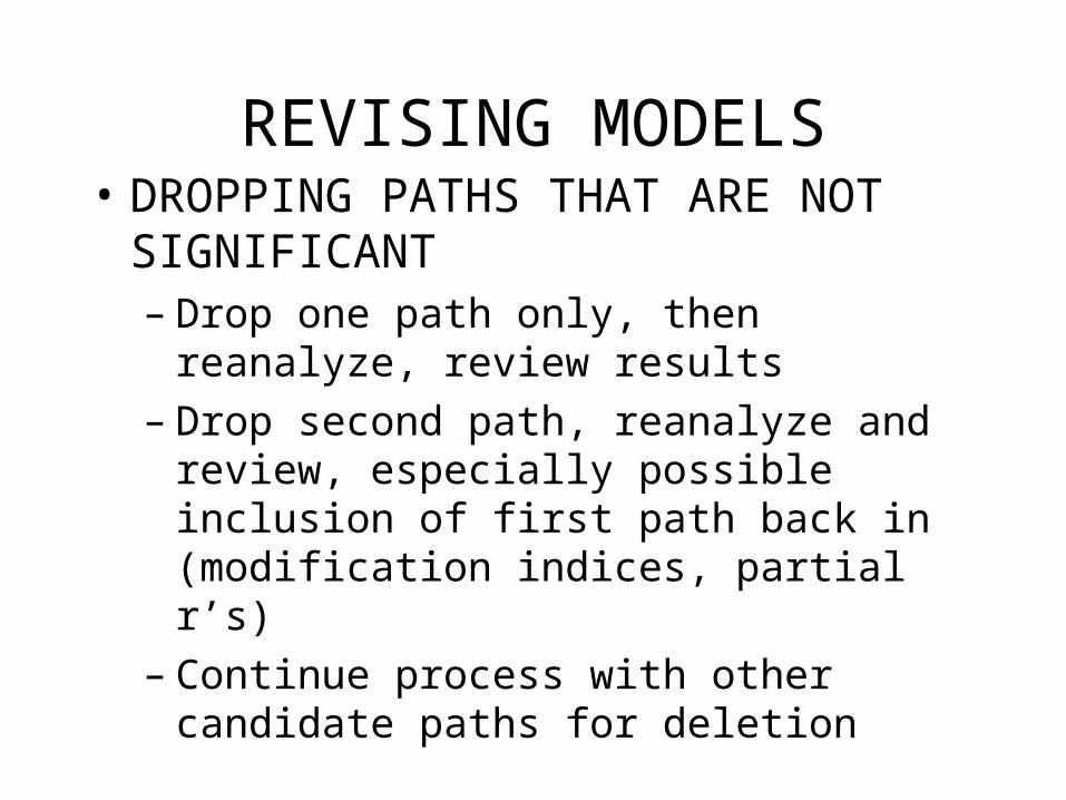
REVISING MODELS• DROPPING PATHS THAT ARE NOT
SIGNIFICANT– Drop one path only, then reanalyze, review
results– Drop second path, reanalyze and review,
especially possible inclusion of first path back in (modification indices, partial r’s)
– Continue process with other candidate paths for deletion

X1
X2
Y e
b = .5
b = .1
r = .4
PATH DIAGRAM FOR REGRESSION
WITH NONSIGNIFICANT PATH
X

X1
X2
Y e
b = .5
r = .4
PATH DIAGRAM FOR REGRESSION
AFTER REMOVING PATH
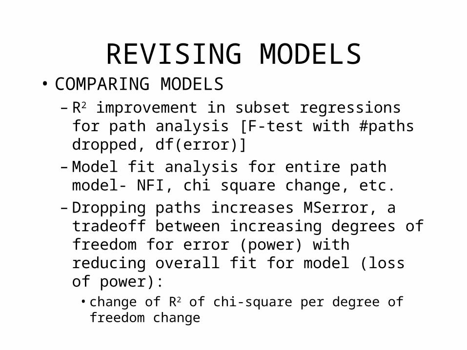
REVISING MODELS• COMPARING MODELS
– R2 improvement in subset regressions for path analysis [F-test with #paths dropped, df(error)]
– Model fit analysis for entire path model- NFI, chi square change, etc.
– Dropping paths increases MSerror, a tradeoff between increasing degrees of freedom for error (power) with reducing overall fit for model (loss of power):
• change of R2 of chi-square per degree of freedom change
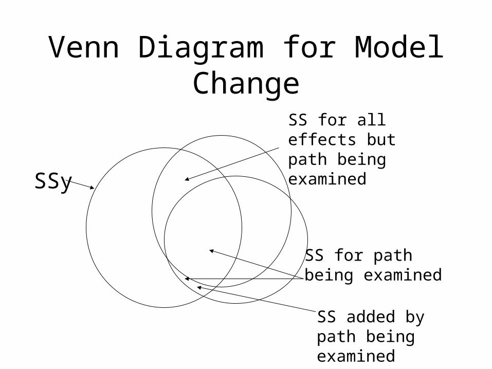
Venn Diagram for Model Change
SSy
SS for all effects but path being examined
SS for path being examined
SS added by path being examined
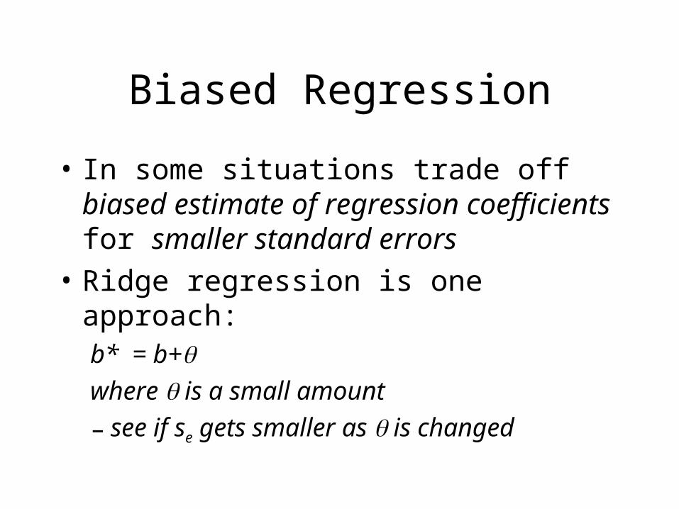
Biased Regression
• In some situations trade off biased estimate of regression coefficients for smaller standard errors
• Ridge regression is one approach:b* = b+where is a small amount
– see if se gets smaller as is changed

MEDIATIONVAR Y MEDIATES THE RELATIONSHIP
BETWEEN X AND Z WHEN1. X and Z are significantly related2. X and Y are significantly related3. Y and Z are significantly related4. The relationship between X and Z is
reduced (partial mediation) or zero (complete mediation) when Y partials the relationship
XY
Z
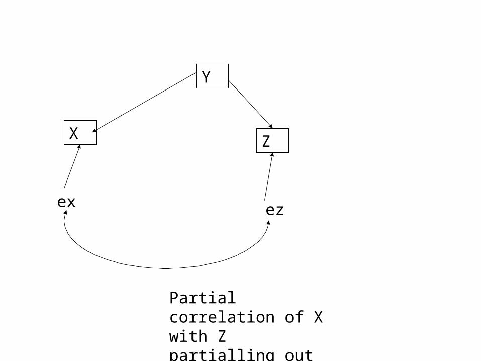
X
Y
Z
ex ez
Partial correlation of X with Z partialling out Y

Z
X
Y
r2XZ.Y

MEDIATION
LOC
SE
DEP
-.448
.512 (.679)
-.373
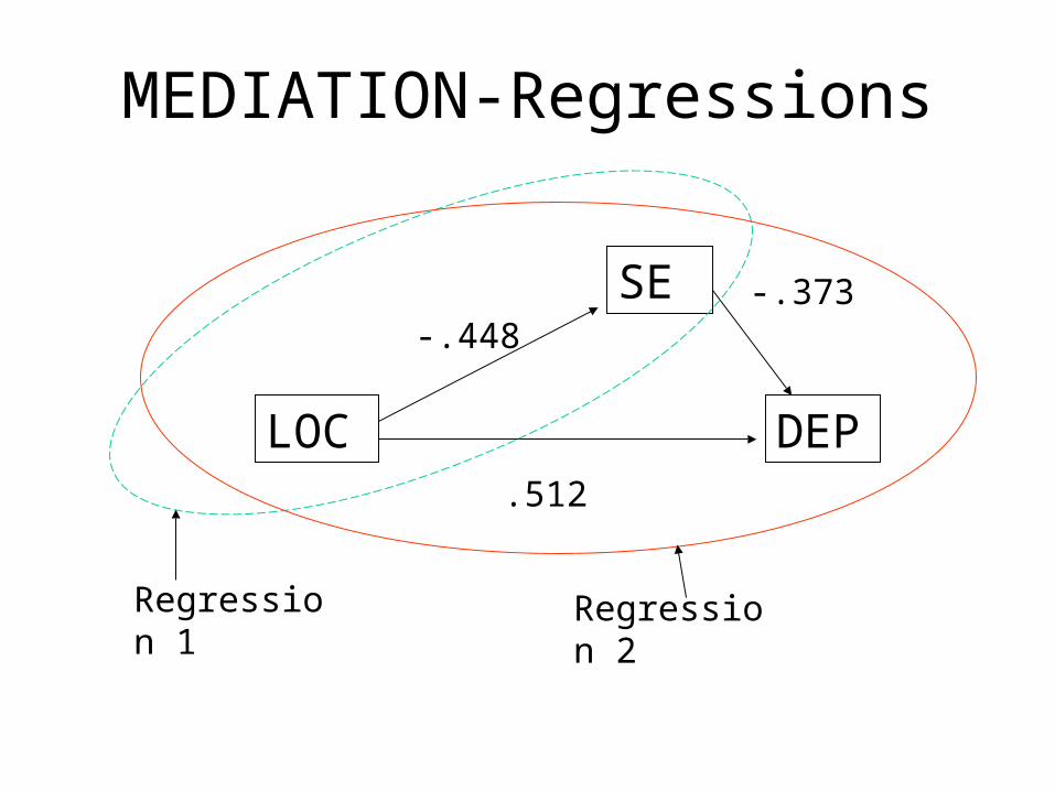
MEDIATION-Regressions
LOC
SE
DEP
-.448
.512
-.373
Regression 1
Regression 2

GENERAL PATH MODELS
LOC
SE
DEP
-.448
.512
-.373Regression 1
Regression 2
ATYPICALITY
Regression 3
.400
.357
R2=.481
R2=.574
R2=.200

GENERAL PATH MODELS
LOC
SE
DEP
-.448*
.512*
-.373*
ATYPICALITY
Regression 3
.394
.320*
R2=.483
R2=.572
R2=.200
-.068 ns

GENERAL PATH MODELS
LOC
SE
DEP
-.448*
.512*
-.373*
ATYPICALITY
Regression 3
.394
.320*
R2=.483
R2=.572
R2=.200
-.068 ns
sex