lecture 14 diagnostics and model checking for logistic regression

Lecture 14Diagnostics and model checking for

logistic regression

BIOST 515

February 19, 2004

BIOST 515, Lecture 14

Outline

• Assessment of model fit

• Residuals

• Influence

• Model selection

• Prediction

BIOST 515, Lecture 14 1

Assessment of model fit – model deviance

The deviance of a fitted model compares the log-likelihood

of the fitted model to the log-likelihood of a model with n

parameters that fits the n observations perfectly. It can be

shown that the likelihood of this saturated model is equal to

1 yielding a log-likelihood equal to 0. Therefore, the deviance

for the logistic regression model is

DEV = −2n∑

i=1

[Yi log(π̂i) + (1− Yi) log(1− π̂i)],

where π̂i is the fitted values for the ith observation. The

smaller the deviance, the closer the fitted value is to the

saturated model. The larger the deviance, the poorer the fit.


Sometimes, you will see a χ2 goodness of fit test based on

the deviance, but this is inappropriate because the number of

parameters in the saturated model is increasing at the same

rate as n.

In the catheterization example,

logit(πi) = β0 + β1sexi has deviance=3217,

logit(πi) = β0 + β1agei has deviance=3153, and

logit(πi) = β0 + β1cad.duri has deviance=3131.

If we had to pick a model with only one predictor, which

might we choose?


Hosmer-Lemeshow goodness of fit test

For this test,

H0 : E[Y ] = exp(X′β)1+exp(X′β)

Ha : E[Y ] 6= exp(X′β)1+exp(X′β).

To calculate the test statistic:

• Order the fitted values

• Group the fitted values in to c classes (c is between 6 and

10) of roughly equal size

• Calculate the observed and expected number in each group

• Perform a χ2 goodness of fit test


Example with catheterization data:

logit(πi) = β0 + β1cad.duri + β2genderi.

1. Order and group the fitted values

>fi1=fitted(glmi1)>fi1c=cut(fi1,br=c(0,quantile(fi1,p=seq(.1,.9,.1)),1))>table(fi1c)

(0,0.371] (0.371,0.422] (0.422,0.426] (0.426,0.433] (0.433,0.442]239 323 180 227 198

(0.442,0.47] (0.47,0.505] (0.505,0.555] (0.555,0.638] (0.638,1]236 230 233 237 229

>fi1c=cut(fi1,br=c(0,quantile(fi1,p=seq(.1,.9,.1)),1),labels=F)>table(fi1c)1 2 3 4 5 6 7 8 9 10

239 323 180 227 198 236 230 233 237 229


2. Calculate the observed and expected values in each group

>E=matrix(0,nrow=10,ncol=2)>O=matrix(0,nrow=10,ncol=2)>for(j in 1:10){> E[j,2]=sum(fi1[fi1c==j])> E[j,1]=sum((1-fi1)[fi1c==j])> O[j,2]=sum(acath$tvdlm[fi1c==j])> O[j,1]=sum((1-acath$tvdlm)[fi1c==j]) }

O E1-Yi Yi 1-pi pi

1 145 94 157.20984 81.790162 219 104 188.94359 134.056413 110 70 103.50988 76.490124 131 96 129.36840 97.631605 111 87 111.13827 86.861736 123 113 128.29642 107.703587 111 119 118.03615 111.963858 95 138 109.43284 123.567169 90 147 95.24991 141.7500910 68 161 61.81471 167.18529


3. Calculate χ2 statistic

X2 =c∑

j=1

1∑k=0

(Ojk − Ejk)2

Ejk∼ χ2

c−2

= 21.56 > 15.5 = χ28,.95;

therefore, we reject H0.

>sum((O-E)^2/E)[1] 21.55852> 1-pchisq(sum((O-E)^2/E),8)[1] 0.005802828


Residuals

Residuals can be useful for identifying potential outliers

(observations not well fit by the model) or misspecified models.

We will look at two types of residuals

• Deviance residuals

• Partial residuals


Deviance residual

The deviance residual is useful for determining if individual

points are not well fit by the model.

The deviance residual for the ith observation is the signed

square root of the contribution of the ith case to the sum for

the model deviance, DEV . For the ith observation, it is given

by

devi = ±{−2[Yi log(π̂i) + (1− Yi) log(1− π̂i)]}1/2,

where the sign is positive when Yi ≥ π̂i and negative otherwise.

You can get the deviance residuals using the function

residuals() in R.


Catheterization example

logit(πi) = β0 + β1cad.duri + β2genderi

●

●

●

●

●

●

●

●

●

●

●

●

●

●●

●●●●

●

●

●

●

●

●

●

●

●

●

●

●

●

●●

●

●

●

●

●

●●

●

●

●

●

●

●●

●

●

●

●

●

●

●●

●

●

●

●

●

●

●

●

●

●

●

●●

●

●

●

●

●

●

●

●

●

●

●

●

●

●

●●

●●

●

●●

●

●

●

●

●●●●

●

●

●

●

●

●

●

●

●

●

●

●

●

●

●

●

●

●●

●

●

●

●

●

●

●

●

●

●

●

●

●

●

●●●

●

●

●

●

●

●●

●

●

●

●

●

●

●●

●

●

●

●

●

●

●●

●

●

●

●●●

●

●

●

●

●

●●

●●

●●●

●

●

●●●●●●

●

●

●●

●

●

●

●

●

●

●

●

●

●

●●●

●●

●

●

●

●

●

●●

●

●

●

●●

●

●

●

●

●

●

●

●

●●●

●

●

●

●

●

●

●

●●

●

●

●

●●●

●

●

●

●

●

●

●●

●

●

●

●●

●

●

●

●

●

●●●

●

●

●

●●

●

●

●●

●

●

●

●●

●

●

●

●

●

●

●●

●

●

●

●●

●

●

●●

●

●

●

●●●

●

●●●●

●

●

●

●●

●

●

●

●

●

●

●

●

●

●

●

●

●

●

●

●

●

●

●

●

●

●

●

●

●●

●

●

●

●

●●

●

●

●

●

●

●

●

●

●

●

●

●

●

●

●

●

●

●

●

●

●

●

●

●

●

●

●

●

●

●

●

●

●

●

●

●

●

●

●

●

●

●●

●

●

●

●

●

●

●

●

●

●

●●

●

●

●●

●

●

●

●●

●●●

●●

●

●

●

●

●

●

●

●

●●●

●

●●

●

●

●

●

●

●

●

●

●

●●

●

●

●

●●

●

●

●

●

●

●

●

●

●

●

●

●●

●

●●

●●

●

●

●

●●

●

●

●

●

●

●

●

●

●

●●

●

●●

●

●

●

●

●

●

●

●

●

●

●

●

●

●●

●

●

●●

●

●

●

●

●●

●

●

●

●

●

●

●

●●

●●●

●

●

●●

●

●

●●

●●

●

●●

●

●●●●

●

●

●

●

●

●●

●

●

●

●●

●

●●

●

●

●

●

●

●

●●●

●

●

●

●

●

●●

●

●

●●

●

●●

●●

●●●

●

●

●

●

●

●

●

●

●●

●●●

●

●

●●

●

●

●

●

●

●

●

●

●●

●

●

●●

●

●

●●

●

●

●

●

●

●

●

●

●

●

●●

●

●

●

●

●

●

●

●●●

●

●

●

●

●

●●

●

●

●●

●

●

●●

●

●●●●

●

●

●

●

●

●

●

●

●●

●

●

●●

●

●

●

●

●●

●●

●●●

●

●

●

●

●

●

●

●

●●

●●

●

●

●

●

●●

●●●

●●●

●

●

●

●●

●

●●

●

●

●

●

●

●

●●

●

●●●

●

●●

●

●

●●

●

●

●

●

●●

●

●

●

●

●

●

●

●●●●●

●●

●

●

●

●

●

●

●

●●

●

●

●

●●

●

●

●

●

●

●

●●

●

●

●●●

●

●

●

●

●●●

●

●

●

●

●

●

●

●

●●

●

●

●●

●

●

●

●

●

●●

●

●

●●

●

●

●

●

●

●●●

●

●●

●

●

●●●

●

●

●

●

●

●

●●●●●

●

●

●●

●

●

●

●

●

●

●

●●●

●

●●

●

●

●●

●●

●

●●

●

●

●●

●

●

●●●

●

●

●

●

●●●

●●

●

●

●

●●

●

●

●

●

●

●●

●●

●

●

●

●

●●

●

●

●

●

●

●

●

●●●

●

●

●●●

●●●

●

●

●

●●

●

●

●●

●●

●

●

●

●

●

●

●

●

●

●

●

●

●

●

●

●●

●

●

●

●

●

●

●

●●●

●

●●

●●

●●

●●

●

●

●

●●

●●

●

●

●

●

●

●

●

●●

●

●

●

●

●

●

●

●

●●

●

●

●

●●

●

●

●

●

●●

●

●

●●

●

●

●

●●

●

●

●

●●●●

●

●●●

●

●●

●●

●

●

●

●●●●

●

●

●

●

●

●●●●●

●

●

●

●

●

●●●

●

●

●●

●

●

●

●

●

●

●

●

●

●

●●

●

●

●

●

●

●

●

●

●

●

●

●

●

●

●

●●●●

●

●

●

●

●

●●

●●

●

●

●

●

●●

●

●

●

●

●

●

●

●

●

●●

●

●●

●

●●

●●●

●

●

●

●●

●●

●●

●

●

●

●

●

●

●

●

●●

●

●

●

●

●●

●

●

●●

●

●

●

●

●

●

●

●

●

●

●

●

●

●

●

●

●

●

●●

●

●●

●●

●

●

●

●

●

●

●●

●

●

●●●

●

●

●●●●●●●●

●

●

●

●

●●

●

●●

●

●

●●

●

●●

●

●

●

●

●

●

●

●

●

●●●

●

●

●

●

●

●●●

●

●

●●

●●

●

●

●

●

●●

●

●

●

●●

●●

●

●●●

●

●

●●●

●

●●

●

●

●

●

●

●

●

●

●

●

●●●

●

●

●●●

●

●

●●●

●

●●

●

●

●●●

●

●

●●

●

●●

●

●

●●

●●

●●

●

●●

●

●

●

●

●

●

●

●

●

●

●

●

●

●●●

●

●

●●●

●

●

●

●

●

●

●

●

●

●

●●●

●

●

●●●

●●

●

●

●

●

●●

●

●

●●

●

●

●

●

●

●

●

●

●

●●●

●

●

●

●

●

●

●

●

●

●

●

●●

●●●

●●

●

●

●

●●

●

●

●

●●●

●

●●●●

●

●

●●

●

●

●

●

●

●

●

●

●

●

●●

●

●

●

●

●

●

●

●

●●●

●

●

●●

●

●

●

●●●

●

●

●

●

●●

●

●

●

●

●

●●

●

●

●

●

●

●

●

●

●●

●

●

●

●

●●●

●

●

●●●

●●●●

●

●

●

●

●●

●

●

●

●

●

●

●

●

●

●

●

●

●●

●

●

●

●

●

●

●

●

●

●

●

●

●

●●

●

●

●

●

●

●

●●

●

●

●

●●●●

●

●●

●

●

●

●

●

●

●●

●

●●●

●

●

●●

●

●

●

●

●

●

●●

●

●

●

●

●

●

●

●●●

●

●

●

●

●

●

●

●●●●●

●

●

●●

●

●

●

●

●

●

●

●

●

●●

●

●●

●●

●

●

●●

●

●●●

●●

●

●

●

●

●

●

●

●

●●●

●

●

●

●

●

●

●

●

●

●●

●●

●

●

●

●●

●

●●

●

●

●

●●●

●

●

●

●●

●●

●

●

●

●

●

●●

●

●

●●

●●

●

●●●

●

●

●●

●

●

●●

●●

●●

●

●

●

●

●

●

●●

●

●

●●

●

●●

●

●

●●●

●●

●

●

●

●

●●

●

●

●

●

●

●

●

●●

●

●

●●●

●

●

●

●

●

●

●

●

●●

●

●

●

●

●

●●●

●

●●

●

●●

●

●

●●●

●

●

●

●

●●

●

●

●●

●●

●

●●

●

●

●

●●

●

●●

●

●

●

●

●

●

●

●●

●

●

●

●●

●

●●●●●

●

●

●

●

●

●

●

●

●

●●

●

●●

●●

●●

●

●

●

●●●●

●

●●

●●

●

●

●

●

●●●

●

●

●

●

●

●

●

●

●

●

●

●

●

●

●●●●

●

●

●

●

●

●

●

●

●

●

●●●

●●●●

●

●

●

●

●

●●●

●

●●●

●

●●

●

●

●●

●

●

●

●

●

●

●

●

●●

●

●

●●

●

●

●

●

●

●

●●●

●

●

●

●

●

●

●

●

●

●

●

●●

●

●

●

●●●

●

●●

●

●

●

●

●

●

●●●

●

●●

●

●●

●●●

●●

●●●

●

●

●●

●●

●

●●

●●

●

●

●

●

●●

●

●

●

●

●

●

●

●

●

●●●●

●

●

●

●

●

●

●

●

●

●

●

●

●

●

●

●●

●

●

●

●●●

●

●

●

●

●

●

●

●

●

●

●●

●

●

●

●●●●

●

●

●

●

●

●●

●

●

●

●

●●

●

●

●

●

●

●●

●

●

●

●●

●

●

●

●

●

●●●

●

●

●

●●

●●●

●

●●●●●

●●

●

●

●

●

●●●●

●

●

●

●

●

●●

●

●

●●

●●●

●

●●

●

●

●

●

●

●

●●●

●●

●

●

●

●

●●

●

●

●

●

●●●●

●

●

●

●

●

●

●

●

●

●●

●

●

●

●

●

●

●

●

●

●

●

●

●

●

●

●●

●

●●

●

●

●

●

●

●

●●

●

●●●

●

●

●

●

●

●

●

●●

●

●

●

●

●

●

●

●

●

●

●

●

●●

●

●

●

●

●●●

●●

●

●

●

●

●

●

●

●

●●

●

●

●

●

●

●

●●

●

●

●

●●●

●●

●

●

●

●●●

●

●

●

●

●

●●

●

●

●

●

●

●

●

●

●

●

●

●

●

●

●●●

●

●

●●

●●

●

●

●

●

●

●

●

●

●

●

●

●●

●

●

●

●

●

●●

●●●

●

●

●

●

●

●

●

●

●

●

●

●

●

●

●

●

●

●

●

●

●

●

●

●

●●

●

●

●

●

●

●

●

●

●●

●●

●

●

0 500 1000 1500 2000

−2.

0−

1.5

−1.

0−

0.5

0.0

0.5

1.0

1.5

index

Dev

ianc

e re

sidu

als


●

●

●

●

●

●

●

●

●

●

●

●

●

●●

●●

●●

●

●

●

●

●

●

●

●

●

●

●

●

●

●●

●

●

●

●

●

●●

●

●

●

●

●

●●

●

●

●

●

●

●

●●

●

●

●

●

●

●

●

●

●

●

●

● ●

●

●

●

●

●

●

●

●

●

●

●

●

●

●

●●

●●

●

●●

●

●

●

●

●●●●

●

●

●

●

●

●

●

●

●

●

●

●

●

●

●

●

●

● ●

●

●

●

●

●

●

●

●

●

●

●

●

●

●

●●

●

●

●

●

●

●

●●

●

●

●

●

●

●

●●

●

●

●

●

●

●

●●

●

●

●

●●●

●

●

●

●

●

●●

●●

●●

●

●

●

●●

●●●●

●

●

●●

●

●

●

●

●

●

●

●

●

●

●●

●

●●

●

●

●

●

●

●●

●

●

●

●●

●

●

●

●

●

●

●

●

●●●

●

●

●

●

●

●

●

●●

●

●

●

●●

●

●

●

●

●

●

●

●●

●

●

●

●●

●

●

●

●

●

●●●

●

●

●

●●

●

●

●●

●

●

●

●●

●

●

●

●

●

●

●●

●

●

●

●●

●

●

●●

●

●

●

●●●

●

●●

● ●

●

●

●

●●

●

●

●

●

●

●

●

●

●

●

●

●

●

●

●

●

●

●

●

●

●

●

●

●

●●

●

●

●

●

●●

●

●

●

●

●

●

●

●

●

●

●

●

●

●

●

●

●

●

●

●

●

●

●

●

●

●

●

●

●

●

●

●

●

●

●

●

●

●

●

●

●

●●

●

●

●

●

●

●

●

●

●

●

●●

●

●

●●

●

●

●

●●

● ●●

●●

●

●

●

●

●

●

●

●

● ●●

●

●●

●

●

●

●

●

●

●

●

●

●●

●

●

●

● ●

●

●

●

●

●

●

●

●

●

●

●

● ●

●

●●

●●

●

●

●

●●

●

●

●

●

●

●

●

●

●

●●

●

●●

●

●

●

●

●

●

●

●

●

●

●

●

●

●●

●

●

● ●

●

●

●

●

●●

●

●

●

●

●

●

●

●●

●●●

●

●

●●

●

●

●●

●●

●

●●

●

●●●

●

●

●

●

●

●

●●

●

●

●

●●

●

● ●

●

●

●

●

●

●

●●

●

●

●

●

●

●

● ●

●

●

●●

●

●●

● ●

● ● ●

●

●

●

●

●

●

●

●

●●

●●●

●

●

●●

●

●

●

●

●

●

●

●

●●

●

●

●●

●

●

● ●

●

●

●

●

●

●

●

●

●

●

● ●

●

●

●

●

●

●

●

●●

●

●

●

●

●

●

●●

●

●

● ●

●

●

●●

●

●●●●

●

●

●

●

●

●

●

●

●●

●

●

● ●

●

●

●

●

●●

●●

●●

●

●

●

●

●

●

●

●

●

●●

●●

●

●

●

●

●●

●●

●

● ●●

●

●

●

●●

●

●●

●

●

●

●

●

●

●●

●

●● ●

●

●●

●

●

●●

●

●

●

●

●●

●

●

●

●

●

●

●

●● ●●●

●●

●

●

●

●

●

●

●

●●

●

●

●

●●

●

●

●

●

●

●

●●

●

●

●●●

●

●

●

●

● ●●

●

●

●

●

●

●

●

●

●●

●

●

●●

●

●

●

●

●

●●

●

●

●●

●

●

●

●

●

● ●●

●

●●

●

●

● ● ●

●

●

●

●

●

●

●●

●●●

●

●

●●

●

●

●

●

●

●

●

●●●

●

● ●

●

●

● ●

●●

●

●●

●

●

●●

●

●

●●●

●

●

●

●

●●●

●●

●

●

●

●●

●

●

●

●

●

● ●

●●

●

●

●

●

●●

●

●

●

●

●

●

●

● ●●

●

●

●● ●

●●●

●

●

●

●●

●

●

●●

●●

●

●

●

●

●

●

●

●

●

●

●

●

●

●

●

●●

●

●

●

●

●

●

●

●●

●

●

●●

●●

●●

●●

●

●

●

●●

●●

●

●

●

●

●

●

●

●●

●

●

●

●

●

●

●

●

●●

●

●

●

●●

●

●

●

●

●●

●

●

●●

●

●

●

●●

●

●

●

●●●●

●

●●●

●

●●

●●

●

●

●

●●● ●

●

●

●

●

●

● ●●●

●

●

●

●

●

●

●●●

●

●

●●

●

●

●

●

●

●

●

●

●

●

●●

●

●

●

●

●

●

●

●

●

●

●

●

●

●

●

●● ●

●

●

●

●

●

●

●●

●●

●

●

●

●

●●

●

●

●

●

●

●

●

●

●

●●

●

● ●

●

● ●

● ●●

●

●

●

●●

●●

●●

●

●

●

●

●

●

●

●

●●

●

●

●

●

●●

●

●

●●

●

●

●

●

●

●

●

●

●

●

●

●

●

●

●

●

●

●

●●

●

●●

●●

●

●

●

●

●

●

●●

●

●

●●●

●

●

●●

●● ●●●●

●

●

●

●

●●

●

● ●

●

●

●●

●

●●

●

●

●

●

●

●

●

●

●

● ● ●

●

●

●

●

●

●●●

●

●

●●

●●

●

●

●

●

●●

●

●

●

● ●

●●

●

●●●

●

●

●●●

●

●●

●

●

●

●

●

●

●

●

●

●

●●●

●

●

●●●

●

●

●● ●

●

●●

●

●

●●●

●

●

●●

●

●●

●

●

●●

●●

●●

●

●●

●

●

●

●

●

●

●

●

●

●

●

●

●

● ●●

●

●

●●●

●

●

●

●

●

●

●

●

●

●

●●●

●

●

●●●

●●

●

●

●

●

●●

●

●

●●

●

●

●

●

●

●

●

●

●

●●●

●

●

●

●

●

●

●

●

●

●

●

●●

●●

●

● ●

●

●

●

● ●

●

●

●

●● ●

●

●●●●

●

●

●●

●

●

●

●

●

●

●

●

●

●

●●

●

●

●

●

●

●

●

●

●●●

●

●

●●

●

●

●

●●●

●

●

●

●

●●

●

●

●

●

●

●●

●

●

●

●

●

●

●

●

●●

●

●

●

●

●● ●

●

●

●●●

●●●

●

●

●

●

●

●●

●

●

●

●

●

●

●

●

●

●

●

●

●●

●

●

●

●

●

●

●

●

●

●

●

●

●

●●

●

●

●

●

●

●

●●

●

●

●

●●●●

●

● ●

●

●

●

●

●

●

●●

●

●●●

●

●

●●

●

●

●

●

●

●

● ●

●

●

●

●

●

●

●

●● ●

●

●

●

●

●

●

●

●●

●●●

●

●

●●

●

●

●

●

●

●

●

●

●

●●

●

●●

●●

●

●

●●

●

●●●

●●

●

●

●

●

●

●

●

●

●●●

●

●

●

●

●

●

●

●

●

●●

●●

●

●

●

●●

●

●●

●

●

●

●● ●

●

●

●

●●

●●

●

●

●

●

●

●●

●

●

●●

●●

●

●●

●

●

●

●●

●

●

● ●

●●

●●

●

●

●

●

●

●

●●

●

●

●●

●

●●

●

●

●●

●

● ●

●

●

●

●

●●

●

●

●

●

●

●

●

● ●

●

●

●●●

●

●

●

●

●

●

●

●

●●

●

●

●

●

●

● ●●

●

●●

●

●●

●

●

●●●

●

●

●

●

●●

●

●

●●

●●

●

●●

●

●

●

●●

●

●●

●

●

●

●

●

●

●

●●

●

●

●

●●

●

●●● ● ●

●

●

●

●

●

●

●

●

●

●●

●

●●

●●

●●

●

●

●

●●● ●

●

●●

●●

●

●

●

●

●●●

●

●

●

●

●

●

●

●

●

●

●

●

●

●

●●● ●

●

●

●

●

●

●

●

●

●

●

●●●

●●●●

●

●

●

●

●

●● ●

●

●●●

●

●●

●

●

●●

●

●

●

●

●

●

●

●

● ●

●

●

●●

●

●

●

●

●

●

●● ●

●

●

●

●

●

●

●

●

●

●

●

●●

●

●

●

●●●

●

●●

●

●

●

●

●

●

●●●

●

●●

●

●●

●●●

●●

●● ●

●

●

●●

●●

●

●●

●●

●

●

●

●

●●

●

●

●

●

●

●

●

●

●

●●●

●

●

●

●

●

●

●

●

●

●

●

●

●

●

●

●

● ●

●

●

●

●●●

●

●

●

●

●

●

●

●

●

●

● ●

●

●

●

●●●●

●

●

●

●

●

●●

●

●

●

●

●●

●

●

●

●

●

●●

●

●

●

●●

●

●

●

●

●

●●●

●

●

●

●●

●●●

●

● ● ●●

●

● ●

●

●

●

●

●●

● ●

●

●

●

●

●

●●

●

●

●●

●●●

●

●●

●

●

●

●

●

●

●●●

●●

●

●

●

●

●●

●

●

●

●

●●● ●

●

●

●

●

●

●

●

●

●

● ●

●

●

●

●

●

●

●

●

●

●

●

●

●

●

●

●●

●

●●

●

●

●

●

●

●

●●

●

●●●

●

●

●

●

●

●

●

●●

●

●

●

●

●

●

●

●

●

●

●

●

●●

●

●

●

●

●● ●

●●

●

●

●

●

●

●

●

●

● ●

●

●

●

●

●

●

●●

●

●

●

●●●

●●

●

●

●

●●●

●

●

●

●

●

● ●

●

●

●

●

●

●

●

●

●

●

●

●

●

●

●●

●

●

●

●●

● ●

●

●

●

●

●

●

●

●

●

●

●

●●

●

●

●

●

●

●●

●●●

●

●

●

●

●

●

●

●

●

●

●

●

●

●

●

●

●

●

●

●

●

●

●

●

●●

●

●

●

●

●

●

●

●

● ●

●●

●

●

0.4 0.5 0.6 0.7 0.8 0.9

−2.

0−

1.5

−1.

0−

0.5

0.0

0.5

1.0

1.5

πi

Dev

ianc

e re

sidu

als


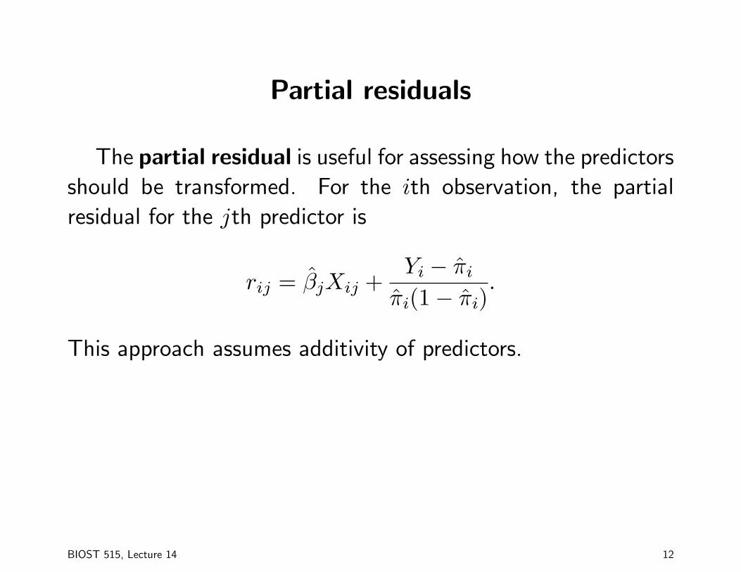
Partial residuals

The partial residual is useful for assessing how the predictors

should be transformed. For the ith observation, the partial

residual for the jth predictor is

rij = β̂jXij +Yi − π̂i

π̂i(1− π̂i).

This approach assumes additivity of predictors.


Influential observations

As in linear regression, we can use DFFITS and

DFBETAS to identify influential observations.

●

●

●●

●

●

●

●

●

●

●

●

●

●●

●●●●

●●●

●

●

●●

●

●●●

●

●

●●

●

●●

●

●●●

●●

●

●●

●●

●

●

●

●

●

●

●●

●

●

●

●●●●

●

●

●

●

●●

●

●

●

●

●

●

●

●●

●

●

●

●

●

●

●

●●

●●●●

●●

●

●●●●

●

●

●

●

●●●

●

●●

●

●●

●●

●

●

●●

●

●●

●

●

●

●

●●

●●

●

●

●●●

●

●

●

●

●

●

●●

●

●

●

●

●

●●●

●

●

●

●

●

●

●●

●

●

●

●●

●

●

●

●

●

●

●

●

●

●

●

●

●

●

●

●●●●

●●●

●

●●

●

●

●●

●

●●

●

●

●

●●

●

●

●

●

●

●

●

●

●●

●

●

●

●

●

●

●

●●

●

●

●

●

●●●

●

●

●

●

●

●

●

●●

●

●

●

●

●●

●

●

●

●●

●

●●

●

●

●

●

●

●

●

●

●

●

●

●

●

●

●

●

●●

●

●

●●●

●

●

●

●

●

●

●

●

●

●

●●●

●

●

●●●

●

●

●

●

●

●

●●●

●

●●

●

●

●

●

●

●●●

●

●

●

●

●

●

●

●

●

●

●

●

●●

●

●

●

●

●

●

●

●

●

●●

●

●

●

●

●●

●

●

●

●

●

●

●

●

●

●

●●●

●

●●

●

●

●

●

●●

●

●

●

●

●

●

●

●

●

●●

●

●●

●

●●

●

●

●●

●●

●

●

●

●

●

●

●

●

●●●

●

●●●

●●

●●●

●●

●●

●●

●●

●

●

●

●

●●

●

●●●

●

●

●

●

●●

●

●

●

●●

●

●

●

●

●

●

●

●

●

●

●

●

●●

●

●

●●

●

●●

●●●

●

●

●●

●

●

●●

●

●

●

●●

●●

●

●

●

●

●

●

●

●●

●

●

●

●

●

●

●

●

●

●

●

●●

●●

●

●

●●

●

●

●

●

●

●

●

●

●

●●●

●

●

●●

●

●

●

●

●●●

●

●

●

●●

●

●

●

●

●●

●

●

●

●

●

●

●

●

●

●

●

●

●

●●

●

●●

●

●

●●

●

●

●

●●

●

●

●●

●

●●

●●

●●●

●

●

●

●

●●●

●

●●

●

●●

●●●●

●

●

●

●

●

●

●

●

●●

●

●

●●

●

●

●●

●

●

●

●

●

●

●

●

●

●

●●

●

●

●

●

●

●

●

●●

●

●

●

●

●

●

●●

●

●

●●

●

●

●

●

●

●●●●

●

●

●

●

●

●

●

●

●●

●

●

●●

●

●

●

●

●●

●●

●●

●

●

●

●

●

●

●

●

●

●●

●

●

●

●●

●●●

●●

●

●●●

●

●

●

●●

●

●●

●

●

●

●

●

●

●●

●

●●●

●

●●

●●

●●

●

●

●

●

●

●

●

●

●●

●

●

●

●●●●●

●●

●

●

●

●

●

●●

●●

●●

●

●

●●

●

●

●●

●

●

●●

●

●●●

●

●

●

●

●

●

●

●

●

●

●

●●

●

●●●●●●●

●

●

●

●

●

●●

●●

●●

●

●●

●

●

●●●

●

●●

●

●

●●●

●

●

●

●

●

●

●●●●

●

●●

●●

●

●

●

●

●

●

●

●●●

●

●●

●

●

●

●

●●

●

●●

●●

●

●

●

●●●●

●

●

●

●

●●●

●●

●

●

●

●●

●

●

●

●

●

●●

●●

●

●

●

●

●

●

●

●

●

●

●

●

●

●●●

●

●

●●●

●●●

●

●

●

●

●

●

●

●●

●●

●

●

●

●

●●

●

●●

●

●

●

●

●

●

●

●

●

●

●

●

●

●

●

●●●

●

●●

●●

●●

●●

●

●

●

●●

●●

●

●●●

●

●

●

●●●●

●

●●

●

●

●

●●

●

●

●●●

●

●

●

●

●●

●

●

●●

●

●●

●

●

●

●

●

●●●●

●

●

●●

●

●●

●

●

●

●

●

●●●●

●●

●●

●

●●●●●

●

●

●

●

●

●●●

●

●

●●

●

●

●●●

●

●●

●

●

●●

●

●

●

●

●

●

●

●

●

●

●

●

●●

●

●●●●

●

●

●

●

●

●●

●●

●

●

●

●

●●●

●

●

●

●

●

●

●

●

●●

●

●●

●

●●

●●●

●

●

●

●●

●●

●

●

●●

●

●

●

●

●

●

●●

●

●

●●

●●

●

●

●●

●●

●

●

●

●

●

●

●

●

●

●

●

●

●

●

●

●

●●

●

●●

●●

●

●●

●

●

●

●●

●

●

●●●

●

●

●●●●●●●●

●

●

●

●

●●

●●●

●

●

●●

●

●●

●

●

●

●

●●

●

●

●

●●●

●

●

●

●●●●●

●

●●

●●●

●

●

●

●

●●

●

●

●

●

●

●

●

●

●●●

●

●

●

●

●

●

●●

●

●

●

●

●

●

●

●

●

●

●●●

●

●

●●●

●

●

●

●

●

●

●●

●

●

●●●

●

●

●

●

●

●●

●

●

●●

●

●

●●

●

●●

●

●

●

●

●●

●

●

●

●

●

●

●

●

●

●

●

●

●●●

●●

●

●

●

●

●

●

●

●

●●●

●

●●

●●

●●

●●

●

●

●●

●●

●●

●●

●

●

●

●

●

●

●●

●●

●

●

●

●

●

●

●

●●

●

●

●●

●●

●

●●

●

●

●

●●

●

●

●

●●

●

●

●●●●

●●

●●

●

●

●

●●

●

●

●

●

●

●

●

●

●

●

●

●

●

●

●

●

●●

●●

●●●

●●

●●●

●

●

●

●

●

●

●

●

●

●

●

●●

●

●●

●

●

●

●

●

●●

●

●

●

●

●●●●●

●●●

●●●

●

●

●

●

●●●

●

●

●

●

●

●

●

●

●

●

●

●

●●

●

●

●

●●

●

●

●●

●

●

●

●

●

●●

●

●

●

●

●

●●

●

●

●

●●●●

●

●●

●

●

●

●

●

●

●●

●

●●●

●

●●

●

●

●

●

●

●

●

●●

●

●

●

●

●

●

●

●●●●●

●

●

●

●

●

●●

●

●●

●

●

●●

●

●

●

●

●

●

●

●

●

●●

●

●●

●●

●

●

●●

●

●●

●

●●

●

●

●

●

●●

●

●

●●●

●

●

●

●

●

●

●

●

●●

●

●●

●

●

●

●●

●

●

●

●●

●

●●●

●

●

●

●●

●●

●

●

●

●

●

●●

●

●

●

●●

●

●

●●

●

●

●

●●

●

●

●●

●●

●●

●

●

●

●

●

●

●●●

●

●●●

●●

●

●

●

●

●

●●

●

●

●

●

●●

●●

●

●

●

●●

●

●

●

●

●●●

●

●

●

●

●●

●

●

●

●

●

●

●

●

●

●●●

●

●●

●

●●

●

●

●●

●

●

●

●●

●

●

●

●

●●

●●

●

●●

●●

●

●●

●

●

●

●

●●

●

●

●

●

●●

●

●

●

●●

●

●●

●

●●

●

●

●

●

●

●

●

●

●

●●

●

●●●

●

●●

●

●

●

●

●●●

●

●●

●●

●

●

●

●

●●●

●

●

●●

●

●●

●

●

●

●●

●

●

●●●●

●

●

●

●

●

●

●

●●

●

●●

●

●●●●

●●

●

●

●

●

●●

●

●●●

●●

●

●

●

●●

●

●

●

●●●

●

●

●●

●

●

●●

●

●

●

●

●

●

●

●●

●

●

●

●●

●

●

●●

●

●

●●

●

●

●

●●●

●

●●

●

●●

●

●

●

●●●

●

●●

●

●●

●●●

●●

●●●

●●

●

●

●●

●

●●

●●

●

●

●

●

●●

●

●

●●

●

●

●

●

●

●

●●●

●

●

●

●

●

●

●●●

●

●

●

●

●●

●●

●●

●

●

●●

●

●

●

●

●

●

●

●

●

●

●●

●

●

●

●●●●

●

●

●

●

●

●

●

●●

●

●

●●

●

●●

●

●

●●

●

●

●●●

●

●

●

●

●

●●●

●

●

●

●●●●●

●

●●

●●

●

●●

●

●

●

●

●

●

●●

●

●

●

●

●

●●

●●

●

●

●●●

●

●

●

●

●

●

●

●

●

●●●

●

●●

●

●

●

●●

●

●

●

●

●●●●

●

●

●

●

●

●

●

●

●●

●

●

●

●●

●

●

●●

●

●

●●●

●

●

●

●

●

●●

●

●

●

●

●

●

●●

●

●●●

●

●●

●

●

●

●

●

●

●

●

●●●

●

●

●●

●

●

●

●

●

●

●

●

●

●

●

●

●●

●

●

●

●

●

●

●

●

●●

●

●

●

●

●

●

●●

●

●

●

●●●

●●

●

●

●

●●●

●

●

●

●

●

●

●●

●

●

●

●

●

●

●

●●●●●

●

●

●●

●

●

●

●

●●

●

●

●●

●

●●●

●

●●

●●

●

●

●

●

●●●

●●●

●

●

●

●●

●

●●●

●

●

●

●●

●

●

●

●

●

●●

●

●●

●●

●●

●

●

●

●

●

●

●●

●

●●

●

0 500 1000 1500 2000

−0.

020.

020.

06

beta 0

Index

dfb[

, i]

●●

●

●●●

●

●

●

●

●

●

●

●●●●●●

●

●

●

●

●●●

●

●

●●

●

●●●●●

●

●●

●●

●

●●●●

●●

●

●

●

●

●●●●●

●

●

●

●●

●●●●

●●●

●●

●

●

●●

●

●

●

●

●●

●

●

●●●●

●

●●

●●

●●●●●●

●

●

●

●●

●

●

●●

●●

●

●

●●●

●

●●

●●

●

●

●●●●

●

●

●

●●

●

●●●

●

●

●

●

●

●●●

●

●

●

●●●●

●●

●

●

●

●

●●

●●

●

●●

●

●●●

●●

●●●●●●●

●●●●●●●●

●

●●●

●

●

●

●

●

●

●

●

●

●

●●●

●●

●●

●

●

●

●●

●

●

●

●

●

●●

●

●

●

●

●

●●●●

●●

●

●

●

●

●

●●

●

●●

●

●●

●

●●

●

●●

●●

●

●

●

●●●

●

●

●

●●●●●

●

●●●

●●●●●●●

●●

●

●

●

●

●

●

●●●

●●●●

●

●●●

●●

●

●●●

●

●●●●●●

●●●●

●●

●

●

●

●

●

●

●

●

●

●

●

●

●●●●●●

●

●

●

●●●●●

●●●

●●●

●

●

●●●●●

●

●

●

●

●

●

●

●

●

●●●

●

●●●●

●●●

●

●

●

●●●

●●

●

●●●●

●●●●●

●

●

●

●

●

●●

●

●

●●

●

●

●

●●

●

●●●●

●

●

●

●

●

●

●●

●●

●

●

●●●

●●●●

●

●

●

●

●●

●

●

●●

●

●

●

●

●

●

●

●●

●●●

●●●●●●●

●

●

●

●●

●

●●

●●

●

●●

●

●●

●

●

●●

●●●

●

●●

●

●

●

●

●

●●●

●●

●●●

●

●

●

●●●●●●●

●

●●

●

●●●●

●

●●

●●

●●●●

●

●●

●●●●●

●

●

●

●●

●●●

●

●

●

●●●●

●

●●

●

●●●●●

●

●●●

●

●●

●●●●●●●

●●

●●●

●

●●●

●●

●

●

●●

●●●●

●

●●

●

●●

●

●

●

●●●●

●

●

●●

●

●

●●●

●

●

●

●

●

●

●

●

●●●

●

●

●

●●●

●

●●●●●

●

●●●●

●

●

●●●●●●

●

●●●●

●

●

●

●●●●

●

●●

●

●

●●●●

●

●

●●●●●●●●

●●

●●

●

●

●

●●●●

●

●

●

●

●●

●●●●●●●●●●●

●

●●●

●

●

●

●

●●●

●

●●●

●

●●

●

●●●●●

●

●

●

●

●

●

●●●●

●

●●●●●●●

●

●

●●

●

●

●●●

●

●

●●●

●

●●

●

●

●●

●

●

●●●●

●●●●●●

●

●

●

●

●●●●

●

●●

●

●

●●

●

●

●●

●●●●●●●●

●

●

●

●●●●

●

●●

●

●

●●●

●

●

●

●

●

●●●●●

●

●●●●

●●

●

●

●

●●●●●

●

●●

●●

●

●●●

●●●●

●

●

●●

●●●●

●

●

●●●●●

●●●

●

●●●

●

●●

●●●●●●

●●

●

●

●●

●

●●

●

●

●

●●●●

●

●●●●

●●●

●

●●

●

●●

●

●●

●●

●

●

●

●

●

●

●●

●

●●

●

●●

●

●●

●

●●●

●

●

●

●●●

●

●●

●●

●●

●●

●

●

●

●●

●●●

●●●●

●

●

●●

●

●

●●

●

●●●

●●

●

●●

●●

●●●

●

●●

●●

●●●

●●●

●

●●

●

●●●●

●●

●●●

●●

●●

●●

●

●●●●

●

●

●

●●●●●●●

●

●

●●●●●●

●

●

●●

●

●●

●

●●

●

●●

●

●●

●

●

●

●

●

●

●

●

●●

●

●

●

●●●●●●

●●

●●●

●●

●●

●●

●

●●●●

●●

●●

●

●

●

●

●●

●

●●

●

●●

●●●

●

●●

●●

●●

●

●●●

●

●●

●

●

●

●●

●

●●

●●●

●●

●●

●

●

●

●●

●●

●●

●

●

●

●●●

●

●

●

●●

●●●

●●

●

●

●●●●●●

●●

●●●

●●

●●●●●●●●

●

●●●●●●

●●●

●●●

●●●

●

●

●

●

●

●●

●●●●●

●●

●

●

●

●●●

●

●

●

●

●●●●

●

●●●

●●

●

●●●●

●●●●

●

●●●

●●

●●●

●

●

●

●

●

●●●

●

●●●

●

●

●●●

●

●

●●●

●

●●

●

●●●●●

●●

●

●

●●●

●

●●

●●●●

●

●●

●

●

●

●

●

●●●●●

●

●

●

●

●

●

●

●

●●●●

●

●●

●●

●●

●●●●●

●

●

●●●

●●●●●

●

●●●

●

●●

●

●

●

●●

●●●

●

●●●

●●●

●

●

●

●

●

●

●

●

●●

●●

●

●●

●●

●

●●●

●●

●●

●●

●●●●●

●

●●

●●

●●

●

●

●●●

●

●

●

●

●

●

●●●

●

●●

●●●●●●

●●

●●●●

●

●●●

●●●●●●●●●●●

●

●

●

●●●●●

●

●●●●●●

●

●

●●●●●●●

●

●

●

●

●●

●●●

●

●

●●

●

●

●●●

●●●

●

●

●

●●●●

●

●●●

●

●●

●

●

●

●

●

●

●●

●●

●

●●●●

●●●

●●●

●●

●

●●

●

●●●

●

●

●●

●

●

●●●

●●●●

●

●●●●

●●●●●

●

●

●

●

●

●●●●●●●

●

●●

●

●●

●

●●●●●●●

●

●●

●●

●

●

●●●

●●

●●●

●

●

●●

●

●●●●●●●

●

●●●

●

●

●●●●

●●

●

●●

●●

●●●●

●

●

●●●

●

●

●●●

●●

●

●●

●●

●●

●

●

●

●●

●

●

●●●●

●

●●

●

●

●●●●

●●●

●

●

●●

●

●●●●●●

●●●

●

●

●

●●

●●●

●

●

●

●●

●

●

●

●

●●●●

●●●

●●●

●●

●

●

●

●●●

●

●

●

●

●●●●●●

●

●●

●

●●

●

●

●●●●

●

●

●

●●●

●●●

●●

●●●

●

●●

●●

●

●

●●●

●

●

●

●

●

●●

●

●

●●●

●

●●●

●●

●

●

●

●

●●

●

●

●

●●

●

●●

●

●

●●●●●

●●●●●●●

●●

●

●●

●●●●

●

●

●●

●

●

●

●

●

●

●

●

●●●●●●

●

●

●●

●

●●

●

●

●

●●

●

●●●●

●

●●●●

●

●●●

●●●●

●●●

●

●●

●●

●

●

●

●●

●

●●

●●

●●

●

●●●

●

●●

●●

●●●●

●

●

●

●

●

●

●

●●

●

●●

●●●●●●

●

●

●

●

●

●

●●●

●

●●

●

●●●●●

●●●●●●

●

●

●

●●

●

●●●●●

●

●

●

●●●●●

●

●

●

●●

●

●●●●

●

●●●

●

●

●

●

●

●

●

●

●

●

●●●

●

●●

●

●●

●

●

●●

●

●

●

●

●●

●●

●●●

●●●●●

●

●

●

●●

●●

●

●

●

●●

●

●●●

●

●●

●

●

●

●●

●

●

●

●●●●●●●

●●●

●●●

●●●

●●

●

●●●●

●●

●●●●●

●

●

●●

●●●

●

●

●●●●

●

●

●

●

●

●

●●

●

●●●

●

●●

●●

●

●●●

●●

●

●●●●

●

●

●●●

●

●●●

●

●

●

●

●

●

●

●

●

●

●●

●

●

●

●

●

●●●●●

●

●

●

●●

●●●●

●●●

●

●

●

●●●

●

●

●

●

●

●

●

●

●●

●

●

●

●

●

●●●●

●

●

●

●●●●●

●

●

●●

●

●●

●●

●●

●

●

●

●●●●●●●●●

●●

●

●

●

●●●●●

●●

●●

●

●

●

●

●

●

●

●●

●

●●●

●

●

●●●●

●

●●

●●

●

●

●

●

●●●●

●

●

●●●

●

●

●

●

●

●●●●●●●●

●

●

●

●

●

●

●

●

●

●

●

●

●

●●●

●

●

●●

●●●

●

●

●

●●

●

●

●

●●●●

●

●

0 500 1000 1500 2000

−0.

15−

0.05

0.05

beta 1

Index

dfb[

, i]

●●

●●

●

●

●

●

●

●

●●●

●●

●●●●

●

●

●

●

●

●

●

●●

●

●

●●

●●

●

●

●

●

●●●

●

●

●

●

●

●●

●●●

●

●

●

●●

●

●

●

●

●

●

●

●

●

●

●

●●

●

●

●

●●

●●

●

●

●

●

●●

●

●●

●●

●

●●

●

●

●

●

●●●●

●●●●●

●

●

●

●

●

●

●

●

●

●

●●

●●

●

●

●●

●

●

●

●

●

●

●

●

●

●

●●

●

●

●

●●

●

●●

●●

●

●●

●

●●

●

●

●

●

●

●

●●●

●

●

●●●

●

●

●

●

●

●

●

●

●

●

●

●

●●

●●●●

●●

●●

●●

●●

●

●

●●

●●

●

●●●●

●

●●

●

●

●

●●●●

●

●●●

●

●

●

●●

●

●

●

●●●

●

●●

●●●

●●●●

●

●

●

●●●

●

●

●

●

●

●●

●

●●●

●

●

●

●●

●

●

●

●

●

●

●

●●

●●

●●

●

●

●●

●

●●●

●

●

●●●

●

●

●

●●

●

●

●●

●

●●●●●

●●●

●

●

●

●●

●●

●

●

●

●●

●

●

●

●

●

●

●●

●

●

●

●

●

●

●

●

●●

●

●●

●

●

●●

●●●

●

●

●

●

●

●

●

●

●●

●

●

●

●

●

●

●

●

●

●

●

●●

●

●

●

●

●

●●

●

●●

●

●

●

●

●

●

●

●●

●

●

●

●

●

●

●

●●

●

●●

●

●

●●

●●

●

●●●

●●

●●

●

●●

●

●●

●

●

●●●

●

●●

●●

●

●

●

●

●

●●●●●●

●

●

●●●

●

●

●

●

●

●

●

●

●

●●

●

●●

●●●●

●●●

●

●●

●

●

●●

●

●

●●●●

●

●

●

●

●●

●

●

●

●●

●

●

●

●

●

●

●

●●

●

●

●●●●

●

●

●

●

●●

●

●●

●●●

●

●●●

●

●

●

●

●●

●

●●●

●●

●

●

●

●

●

●

●●●

●

●●

●

●

●

●

●

●

●

●

●

●

●

●

●●●

●

●

●

●

●●

●

●

●●

●

●●

●●

●●●

●

●

●●●●

●●

●●

●●●

●

●

●●

●

●

●●

●

●

●

●

●●

●

●

●●

●●●●

●

●●●

●●

●

●●

●

●●●

●

●

●

●

●

●

●●

●

●

●

●●

●

●●

●

●

●●

●

●

●●

●●●●●●

●●●

●

●

●

●

●●

●

●

●●

●

●

●

●

●●

●●

●●●

●

●

●●

●●

●

●

●●

●●

●

●

●

●●●

●●●

●●●

●

●

●

●●

●

●●

●●

●

●

●●

●●●

●●●

●

●●

●

●

●●

●

●

●●●

●

●

●

●●

●

●

●

●●●●●

●●●●

●

●

●

●

●

●●●

●

●

●●

●

●

●

●●●

●

●

●●

●●●

●

●

●

●

●

●

●

●●

●

●

●

●

●

●

●●

●

●●●

●●

●

●●

●●

●●

●●

●

●

●●●

●●●

●

●●

●●●●●●

●

●

●

●

●

●●●●

●

●

●

●●

●

●

●●

●

●

●

●●●

●

●●

●

●

●

●

●●

●

●●

●

●●

●

●

●●●●

●●●

●

●●●●●●

●●

●●

●●

●

●

●

●●

●●

●

●

●

●●●●

●

●●

●●●

●●●

●●

●●●●●●●

●

●

●●

●●

●●

●●

●

●

●

●●

●

●

●

●●

●

●

●

●

●●●●

●

●

●●

●

●

●●●

●●●●●●●●●

●

●●

●●

●●

●

●

●

●

●

●

●●●

●

●

●

●

●●

●

●

●●

●

●

●

●●

●

●

●

●

●●●

●

●●

●●●

●●●

●

●

●●●●●

●

●●

●

●●●●●

●●

●●●●●

●

●

●

●

●●●●●●

●

●

●

●

●●●

●

●

●●●

●

●

●

●

●

●●

●●

●●

●●●

●

●

●

●

●

●

●●

●

●

●

●

●●●●

●

●

●

●

●

●●

●●●

●●●

●●●

●

●

●

●

●

●

●

●

●●

●

●●●●●

●●●

●

●

●●●

●●

●●

●

●

●●

●

●●

●

●●●●

●

●

●●

●

●

●●

●

●

●●

●

●

●●

●

●

●

●

●

●

●●

●●●●●

●●

●●●

●

●

●

●

●

●●

●

●

●●●●●

●●●●●●●●

●

●

●

●

●●

●●●

●●

●●

●

●●

●

●

●

●●

●

●

●

●

●●●●

●

●

●

●

●●●

●

●

●

●

●●

●

●

●

●

●●

●

●

●●

●

●●●

●●●

●●

●

●

●

●

●●

●

●

●

●

●

●

●

●

●

●●●●

●●

●●●

●●

●

●

●

●

●●●

●

●●●

●●

●

●

●●●

●

●

●●

●●

●●

●

●●

●●

●

●

●

●

●

●

●

●

●

●●●

●

●

●●●●●

●

●●

●

●

●●

●

●

●

●●●●

●

●

●●

●●

●

●

●

●

●●

●

●

●●

●

●●

●

●

●

●

●

●

●●●●

●

●

●●●●

●

●

●

●

●●

●●

●

●●

●

●●●●

●●

●●●

●

●

●●●●

●

●

●●

●

●

●

●

●●●

●

●●●

●

●

●

●

●

●

●

●●

●

●●

●

●

●●●

●

●

●●●

●

●

●

●●●

●

●

●

●

●

●●

●

●

●

●

●

●

●

●

●●

●●

●

●

●●●●●●●●

●●●●●

●

●

●

●●

●

●

●

●

●

●

●

●

●

●

●

●●●

●●

●●

●

●

●

●

●

●

●

●●●

●

●

●

●

●●

●

●●●

●

●

●●●●

●

●●

●

●

●●

●

●

●●

●

●●●

●

●

●

●

●

●●

●

●

●

●●

●●●

●

●

●●

●●●●●

●●

●

●●

●●

●

●●

●

●●●

●●

●●●

●

●

●

●

●●

●

●●

●●

●

●

●●

●

●●●

●●

●

●

●

●

●

●

●

●

●●●

●

●

●

●

●●

●

●

●

●

●

●●

●●

●

●●

●

●

●

●

●

●

●●●●●

●

●●

●●

●

●

●

●

●

●●

●

●

●

●

●

●

●

●●

●

●

●

●●

●

●

●●

●●

●●

●

●

●

●

●

●

●●●

●

●●●

●●●●●●●

●●

●●●

●

●●

●

●

●

●

●

●

●

●

●

●

●●●●

●

●

●●

●

●

●

●●

●●

●

●

●

●

●●●

●

●●

●

●●

●

●

●●

●

●●

●

●●●

●

●

●●●●

●

●●

●

●

●

●●

●

●

●

●

●

●●

●●

●

●●

●

●

●

●●

●

●●

●

●●

●

●●●●

●

●●

●

●●

●

●●●

●

●●

●

●

●

●

●●●

●

●●

●●

●●

●

●

●●●

●

●

●

●

●●

●

●

●

●●

●

●

●

●●●●

●

●

●

●●●

●●

●

●●●

●

●●●●

●

●

●

●

●●

●●

●

●●●

●

●●

●●

●●

●

●●●

●

●

●

●

●●

●

●●●●

●

●●●

●

●

●●

●

●

●

●

●

●

●

●

●●●●●

●

●

●●●●

●

●●

●

●●

●

●

●

●●●

●

●●

●

●●

●●●

●●

●●●

●

●

●●

●●

●

●●

●●

●

●

●

●●●

●

●

●

●●

●

●

●●

●●●●

●●

●

●

●

●

●

●

●●

●

●

●

●

●

●●

●●

●●

●●

●●●

●

●

●●●

●

●●●

●

●

●

●●●●

●

●

●

●

●

●

●

●

●

●

●

●●

●

●

●

●

●

●●

●

●●

●●●

●

●

●

●

●●●

●

●

●

●●●●●

●

●●

●●

●●●

●

●

●

●

●

●

●●

●

●

●●

●

●●

●

●

●

●

●●●

●

●

●●●●●

●

●

●●●

●

●

●

●

●

●

●●

●●

●

●

●●●●●●●

●

●

●

●

●

●

●

●

●●●

●

●●

●

●

●

●●

●

●

●

●

●

●

●

●●

●

●●

●

●

●

●●

●●●●●●●

●

●

●

●

●

●

●

●

●

●

●●

●●

●●

●

●

●

●

●

●

●

●

●

●

●

●●

●●●

●

●●●

●●●

●

●●

●

●

●

●●

●

●

●

●●●

●●

●

●

●

●●●

●

●

●

●

●

●

●

●●

●

●

●●●

●

●

●

●

●

●

●

●

●●

●

●●

●

●●

●●

●

●

●

●

●

●

●

●

●

●●●●

●

●●

●●

●●●

●

●

●

●

●●●

●

●

●

●

●●

●

●

●

●

●●

●

●

●

●

●

●●

●

●

●

●

●

●

●

●

●●

●

●

●

●

0 500 1000 1500 2000

−0.

040.

000.

04

beta 2

Index

dfb[

, i]

●●

●●

●

●

●

●

●

●

●●●

●●

●●●●

●●●

●

●●

●

●●

●

●

●●

●●

●

●

●

●

●●●

●

●

●●

●

●●

●●●

●

●

●●●●

●

●

●●

●

●

●

●

●

●

●●

●

●●

●●

●

●

●

●

●

●

●●

●

●●

●●

●

●●

●●

●

●

●●●●

●●●●●

●●

●

●

●

●

●

●

●

●

●●

●●

●

●

●●

●●●

●

●

●

●

●

●

●

●●●

●●

●

●

●

●●

●●

●

●●

●

●●

●

●

●●

●

●

●●●

●

●

●●●

●

●

●

●

●

●●

●

●

●

●

●

●●

●●●●●●

●●

●●

●●

●●

●●

●

●

●

●●●●

●

●●●

●

●

●●●●

●

●●●

●

●

●

●●

●

●

●

●●●

●

●●

●

●

●

●●●●

●

●

●

●●●

●

●

●

●

●

●●

●

●

●

●●●

●

●

●

●

●●

●●

●

●●●

●●

●●

●

●

●●

●

●●●

●●

●●●

●

●●●●

●

●

●●

●●

●

●●●

●●●

●

●

●

●●

●●

●

●

●

●●

●

●

●

●

●

●

●●

●

●

●

●

●

●

●

●

●●

●

●●

●

●

●●

●●●

●

●

●

●

●

●

●

●

●

●

●

●

●

●

●

●

●

●

●

●

●

●

●

●

●

●

●

●

●●

●

●

●●

●

●●

●

●

●

●●

●

●

●

●

●

●

●

●●

●

●●

●

●

●●

●●

●

●●●

●●

●●

●

●●

●

●●

●●

●●●

●

●●

●●

●

●

●

●

●

●●●●●●

●●

●

●

●

●

●

●

●

●

●

●●●

●●

●

●●

●●●●

●●●

●

●●

●

●

●●

●

●

●●●●

●

●

●●●

●●

●

●

●●

●

●

●●●

●

●

●●

●

●

●

●

●●

●

●●●

●●

●

●●

●●●

●

●●●

●

●

●●

●●

●

●●●

●●●●

●

●

●

●

●●●

●

●●

●

●

●

●

●

●

●

●

●

●●

●

●●●

●

●

●

●

●●

●●●●

●

●●

●●

●●●

●

●

●●●●

●●

●●

●●●

●

●

●●

●

●

●●

●

●

●

●

●●

●

●

●●

●●●●

●

●

●

●

●●

●

●●

●

●●●

●

●

●

●

●

●

●●●

●

●

●●

●

●●

●

●

●●

●

●

●●

●

●●●●

●

●●●

●

●

●

●

●●

●

●

●●

●

●

●

●

●●●●

●●●

●

●

●●

●●

●

●

●●

●●

●

●

●

●●●

●●●

●●●

●

●

●

●●

●

●●

●●

●●

●●

●●

●

●●●

●

●●

●

●

●●

●

●

●●●

●

●

●

●●●

●

●

●●●●●

●●●●

●

●

●

●

●●●

●

●

●

●●

●

●

●

●●●

●

●

●●

●●●

●●●

●

●●

●

●●

●

●

●

●

●

●●●

●

●●●

●●

●

●●

●●●●

●●

●●

●●●

●●●

●

●●

●●●●●●

●

●

●

●

●

●●●●

●

●

●●●

●

●

●

●

●

●

●

●●●

●

●●

●

●

●

●

●●

●

●●

●

●●

●

●

●●●●

●●●

●

●●●●●●

●●●●

●●

●

●

●

●●

●●

●

●

●

●●●●

●●●

●●●

●●●

●●

●●●●●●●

●

●

●●

●●

●●

●●

●

●

●

●●

●

●

●

●●

●

●

●●

●●●●

●●

●●

●

●

●●●

●●●●●●●●●

●

●●

●●

●●

●

●

●

●●

●

●

●●●

●

●

●

●●

●

●

●●

●

●

●

●●

●

●

●

●

●●●

●

●●

●●●

●●●

●

●

●●●●●●

●●●

●●●●●

●

●

●●●●●

●●

●

●●●●●●●

●

●●

●

●●●

●

●

●●●

●

●

●

●

●●●

●●

●●

●●●

●

●

●

●

●

●

●●

●

●

●

●

●●●●

●

●●●●

●●

●●●

●●●

●●●

●

●●●

●

●

●

●

●●

●

●●●●●

●●●

●

●

●●●

●●

●●

●

●

●●

●

●●

●

●●●●

●

●

●●

●

●

●●

●

●

●●

●

●

●●

●

●

●

●

●●●

●

●●●●●

●●

●●●

●●●●

●

●●

●

●

●●●●●

●●●●●●●●

●

●●●

●●

●●●

●●

●●

●

●●

●

●

●

●●

●

●

●

●

●●●●

●

●

●

●

●●●

●

●

●

●

●●

●●●●●●

●

●●●

●

●●●

●●●

●●

●●

●

●

●●

●

●

●

●

●

●

●

●●

●

●●●

●●

●●●

●●

●

●●

●

●●

●●●●●

●●

●

●

●●●

●

●

●●

●●

●●

●

●●

●●

●

●

●

●

●

●

●●

●

●●●

●

●

●●●●●

●

●●

●

●

●●

●

●

●

●●●●

●

●

●●

●●

●

●

●

●

●●

●

●

●●

●

●●

●

●

●

●

●

●

●●●●

●

●

●

●

●

●

●

●

●

●

●●

●●

●

●●

●●●●●

●●

●●●

●

●

●●●●

●

●

●●

●

●

●

●

●

●●

●

●●●

●

●

●

●

●●●

●●

●

●●●

●

●●●

●

●

●●●

●

●●

●●●

●●

●

●●●●●

●

●

●

●

●

●

●●●

●●

●●●●●●●●●●

●●●●●

●

●

●

●●

●

●

●

●

●

●

●

●

●

●

●

●●●

●●

●●

●

●

●

●●

●

●

●

●

●●

●

●

●

●

●

●

●●●

●

●

●●●●

●●●

●

●

●●

●●

●●

●

●●●

●

●

●

●

●

●●

●

●

●

●●

●

●

●

●

●

●●

●●●●●

●●

●

●●

●●

●●●●

●●●

●●

●●●

●

●

●

●

●●

●

●●

●●

●

●

●●●

●●●

●●

●

●

●

●●●

●

●●●●

●

●

●

●

●●

●

●

●

●

●

●●

●●

●

●●

●

●

●

●

●

●

●●●●●

●

●●

●●

●

●●

●

●

●●

●

●

●

●

●

●

●

●●

●

●

●

●●●●

●●

●●

●●

●

●

●

●

●

●

●●●

●

●●●

●●●●●●●

●●

●●●

●

●●

●●

●

●

●

●

●●

●

●

●●●●

●

●

●●

●

●

●

●●

●●

●

●

●

●

●●●

●

●●

●

●●

●

●

●●

●

●

●

●

●●●

●

●

●●●●

●

●●

●

●

●

●●

●

●

●

●●

●●

●

●

●

●●

●

●

●●●

●

●●

●

●●

●

●●

●

●●

●●

●

●●

●●●●

●

●●

●

●●

●

●●●

●

●●

●●

●●

●

●

●●●

●

●

●

●

●

●●

●

●

●●

●

●

●

●●●●

●

●

●

●●●

●●

●

●●●

●

●●●●

●

●

●●

●●

●●

●

●●●

●

●●

●●

●●

●

●●●

●

●

●

●

●●

●

●●●●

●

●●●

●

●

●●

●●

●

●

●

●

●

●

●●●●●

●

●

●●●●

●

●●

●

●●

●

●

●

●●●

●

●●

●

●●

●●●

●●

●●●

●●

●●

●●

●

●●●●●

●

●

●●●

●●

●

●

●

●

●●●

●●●●

●●

●

●

●

●

●

●●

●

●

●

●

●●

●●●

●●●

●●

●●●

●

●

●●●

●

●●●

●

●

●

●●●●

●

●●

●

●

●

●

●

●

●

●

●●

●

●

●

●

●

●●

●

●●

●●●

●

●

●

●●●●

●

●

●

●●●●●

●

●●

●●

●●●

●●

●

●

●●●●●

●

●●

●

●●

●

●

●

●

●●●

●

●

●●●●●

●

●

●●●

●

●

●

●

●

●

●●

●●

●

●

●●●●

●

●●

●

●

●

●

●

●

●

●

●●●

●

●●

●

●

●

●●

●

●

●

●

●●●

●●

●

●●

●

●

●

●●

●●●●●●●

●

●

●

●

●

●

●

●

●

●

●●

●●

●●

●

●

●

●

●

●

●

●

●

●

●

●●

●

●

●

●

●●●

●●●

●

●

●

●

●

●

●●

●

●●●●●

●●

●

●

●

●●●

●

●

●

●

●

●

●

●●

●

●

●

●

●

●

●●

●

●

●

●

●

●●●

●●

●

●●

●●

●

●

●●

●

●

●

●

●

●●●●

●

●●

●●●●●●

●

●

●

●

●●●

●

●

●

●

●

●

●

●

●

●●

●

●

●

●

●

●●

●

●

●

●●

●

●

●

●●●●

●

●

0 500 1000 1500 2000

−0.

15−

0.05

0.05

DFFITS

Index

dffit

s(gl

mi1

)


The potentially influential observations we’ve identified are:

sex age cad.dur choleste sigdz tvdlm314 1 63 364 350 1 01239 1 61 349 250 1 0

As it turns out, these are the two most extreme observations

in duration for males without severe coronary artery disease.


acath$cad.dur

● ●● ●●● ●●●● ● ●● ●● ●● ●●● ●● ●● ●●●●●● ●● ●● ● ●●●● ●● ●●● ●●●● ● ●● ● ●● ●● ●● ● ●● ●● ●●● ● ●●● ●● ●●● ● ●● ●● ● ●●●● ●● ●● ● ●●

● ● ● ●●● ●●●●● ●●● ● ●●

Female

Male

0 100 200 300 400

Not severe

● ●●●●● ●●●● ●●●● ●● ●● ●●●● ● ● ●● ●●● ●●● ●●● ●●

● ● ●● ● ● ●● ●● ●● ●● ●● ● ●

Severe

0 100 200 300 400


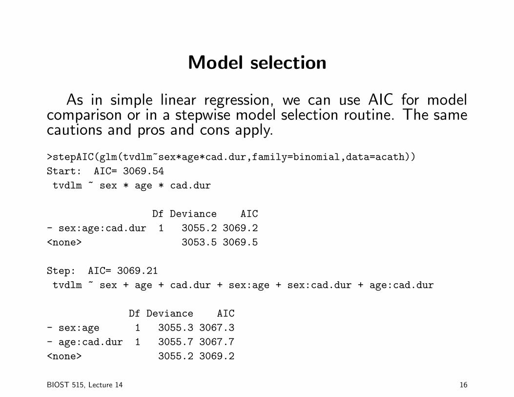
Model selection

As in simple linear regression, we can use AIC for modelcomparison or in a stepwise model selection routine. The samecautions and pros and cons apply.

>stepAIC(glm(tvdlm~sex*age*cad.dur,family=binomial,data=acath))Start: AIC= 3069.54tvdlm ~ sex * age * cad.dur

Df Deviance AIC- sex:age:cad.dur 1 3055.2 3069.2<none> 3053.5 3069.5

Step: AIC= 3069.21tvdlm ~ sex + age + cad.dur + sex:age + sex:cad.dur + age:cad.dur

Df Deviance AIC- sex:age 1 3055.3 3067.3- age:cad.dur 1 3055.7 3067.7<none> 3055.2 3069.2


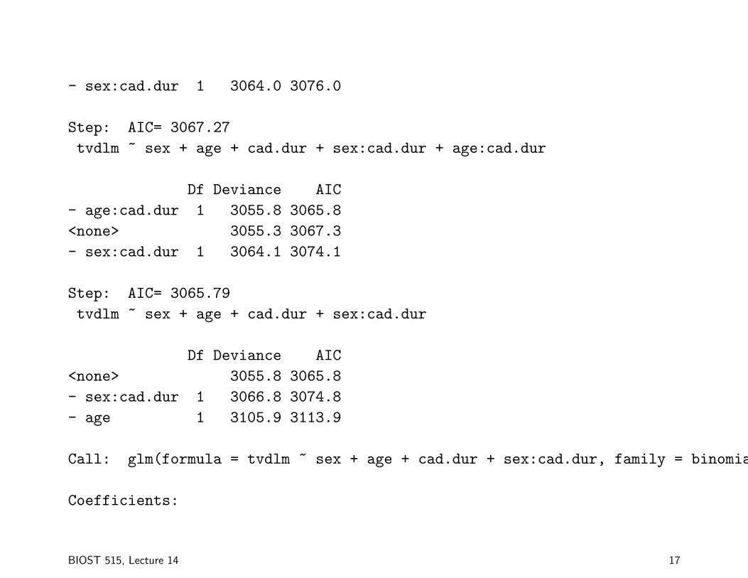
- sex:cad.dur 1 3064.0 3076.0

Step: AIC= 3067.27tvdlm ~ sex + age + cad.dur + sex:cad.dur + age:cad.dur

Df Deviance AIC- age:cad.dur 1 3055.8 3065.8<none> 3055.3 3067.3- sex:cad.dur 1 3064.1 3074.1

Step: AIC= 3065.79tvdlm ~ sex + age + cad.dur + sex:cad.dur

Df Deviance AIC<none> 3055.8 3065.8- sex:cad.dur 1 3066.8 3074.8- age 1 3105.9 3113.9

Call: glm(formula = tvdlm ~ sex + age + cad.dur + sex:cad.dur, family = binomial, data = acath)

Coefficients:


(Intercept) sex age cad.dur sex:cad.dur-2.124102 -0.265944 0.034020 0.007418 -0.006221

Degrees of Freedom: 2331 Total (i.e. Null); 2327 ResidualNull Deviance: 3230Residual Deviance: 3056 AIC: 3066


Starting with intercept only model

> stepAIC(glm(tvdlm~-1+1,data=acath,family=binomial),scope=~sex*age*cad.dur)Start: AIC= 3232.49tvdlm ~ -1 + 1

Df Deviance AIC+ cad.dur 1 3131.3 3135.3+ age 1 3153.0 3157.0+ sex 1 3217.0 3221.0<none> 3230.5 3232.5

Step: AIC= 3135.26tvdlm ~ cad.dur

Df Deviance AIC+ age 1 3091.3 3097.3+ sex 1 3117.9 3123.9<none> 3131.3 3135.3- cad.dur 1 3230.5 3232.5


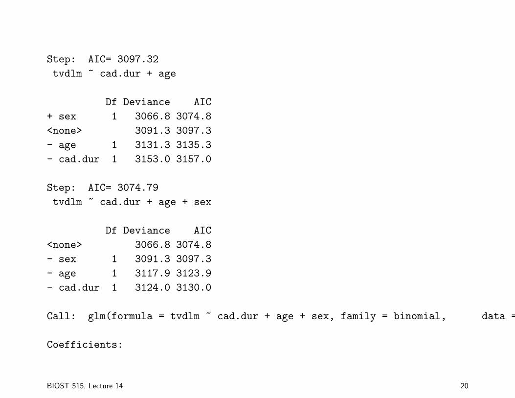
Step: AIC= 3097.32tvdlm ~ cad.dur + age

Df Deviance AIC+ sex 1 3066.8 3074.8<none> 3091.3 3097.3- age 1 3131.3 3135.3- cad.dur 1 3153.0 3157.0

Step: AIC= 3074.79tvdlm ~ cad.dur + age + sex

Df Deviance AIC<none> 3066.8 3074.8- sex 1 3091.3 3097.3- age 1 3117.9 3123.9- cad.dur 1 3124.0 3130.0

Call: glm(formula = tvdlm ~ cad.dur + age + sex, family = binomial, data = acath)

Coefficients:


(Intercept) cad.dur age sex-2.079777 0.005957 0.034330 -0.546153

Degrees of Freedom: 2331 Total (i.e. Null); 2328 ResidualNull Deviance: 3230Residual Deviance: 3067 AIC: 3075

Which model do we prefer?


Prediction

An main interest of logistic regression is often prediction.

Given that we estimate probabilities for individuals, how can

we translate this into a predicted outcome?

Two possibilities for prediction rules are:

1. Use 0.5 as a cutoff. That is if π̂ for a new observation is

greater than 0.5, its predicted outcome is y = 1. Otherwise,

it’s y = 0. This approach is reasonable when

(a) it is equally likely in the population of interest that the

outcomes 0 and 1 will occur, and

(b) the costs of incorrectly predicting 0 and 1 are approximately

the same.


2. Find the best cutoff for the data set on which the multiple

logistic regression model is based. Using this approach, we

evaluate different cutoff values and for each cutoff value,

calculate the proportion of observations that are incorrectly

predicted. We would then select the cutoff value that

minimizes the proportion of incorrectly predicted outcomes.

This approach is reasonable when

(a) the data set is a random sample from the population of

interest, and

(b) the costs of incorrectly predicting 0 and 1 are the same.


In the catheterization example,

logit(πi) = β0 + β1cad.duri + β2genderi,

if we use the cutoff of 0.5, we get the following results

> table(fitted(glmi1)>.5,acath$tvdlm)

0 1FALSE 937 674TRUE 266 455

>t1=table(fitted(glmi1)>.5,acath$tvdlm)>(t1[2,1]+t1[1,2])/sum(t1)0.4030875

So, we misclassify people 40% of the time.Instead, let’s try finding a classification rule that minimizesmisclassification in our data set.

> for(p in seq(.35,.9,.05)){+ t1=table(fitted(glmi1)>p,acath$tvdlm)


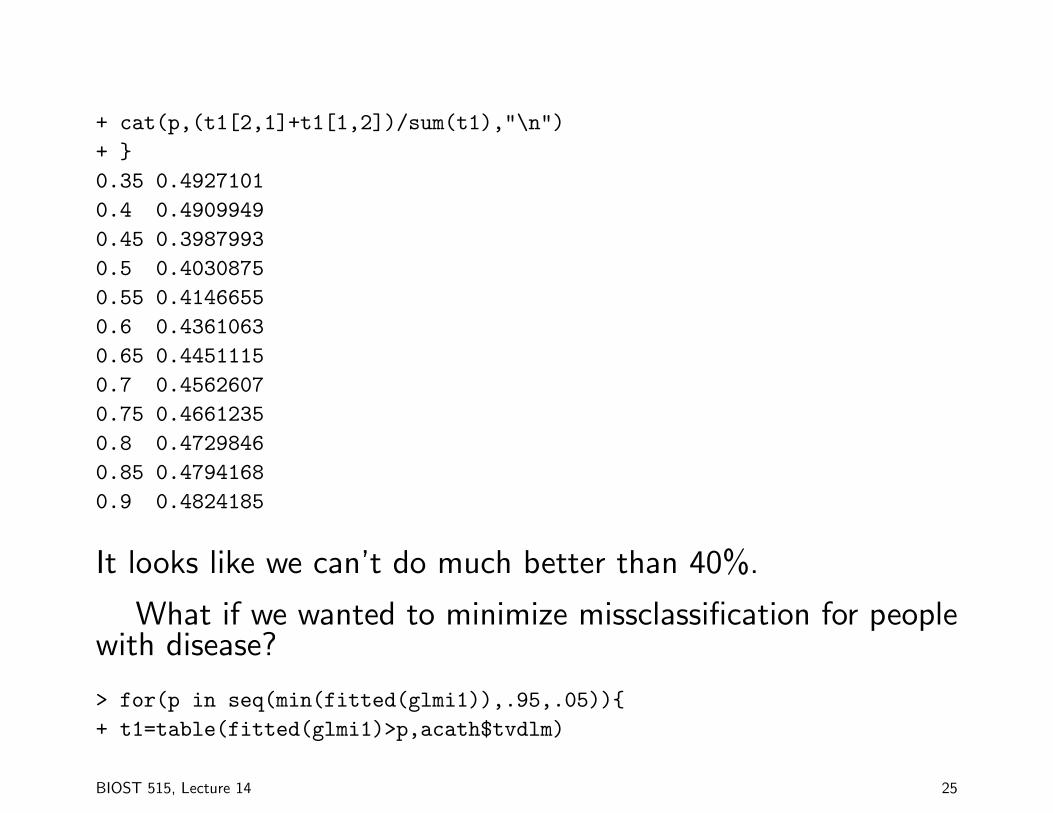
+ cat(p,(t1[2,1]+t1[1,2])/sum(t1),"\n")+ }0.35 0.49271010.4 0.49099490.45 0.39879930.5 0.40308750.55 0.41466550.6 0.43610630.65 0.44511150.7 0.45626070.75 0.46612350.8 0.47298460.85 0.47941680.9 0.4824185

It looks like we can’t do much better than 40%.

What if we wanted to minimize missclassification for peoplewith disease?

> for(p in seq(min(fitted(glmi1)),.95,.05)){+ t1=table(fitted(glmi1)>p,acath$tvdlm)


+ cat(p,(t1[1,2])/sum(acath$tvdlm),(t1[2,1])/sum(1-acath$tvdlm),"\n")+ }0.329234 0.005314438 0.99251870.379234 0.08857396 0.87032420.429234 0.2604074 0.56525350.479234 0.5323295 0.27514550.529234 0.6589903 0.17040730.579234 0.765279 0.10806320.629234 0.8379097 0.068994180.679234 0.8990257 0.037406480.729234 0.9326838 0.019950120.779234 0.9619132 0.0066500420.829234 0.9822852 0.0041562760.879234 0.9911426 0.00083125520.929234 0.9991143 0


Quantifying predictive ability

Similar to the approach above we can plot the receiveroperating characteristic (ROC) curve. This curve is a plot

of 1-specificity against sensitivity.

We can plot this with a slight modification of the codeabove.

p1=matrix(0,nrow=13,ncol=3)i=1for(p in seq(min(fitted(glmi1)),.95,.05)){t1=table(fitted(glmi1)>p,acath$tvdlm)p1[i,]=c(p,(t1[2,2])/sum(t1[,2]),(t1[1,1])/sum(t1[,1]))i=i+1}plot(1-p1[,3],p1[,2])


●

●

●

●

●

●

●

●

●●●●●

0.0 0.2 0.4 0.6 0.8 1.0

0.0

0.2

0.4

0.6

0.8

1.0

1−specificity

sens

itivi

ty


The area under the ROC curve can give us insight into the

predictive ability of the model. If it is equal to 0.5, the model

can be thought of as predicting at random (an ROC curve with

slope = 1). Values close to 1 indicate that the model has good

predictive ability.

A similar measure is Somers’ Dxy rank correlation between

predicted probabilities and observed outcomes. It is given by

Dxy = 2(c− 0.5),

where c is the area under the ROC curve. When Dxy = 0,

the model is making random predictions. When Dxy = 1, the

model discriminates perfectly.


We can get this Dxy and c value by using the somers2()function in the Hmisc library in R.

> somers2(fitted(glmi1),acath$tvdlm)C Dxy n Missing

0.6293747 0.2587493 2332.0000000 0.0000000

So, the area under the ROC curve is 0.629, and Dxy = 0.26.


What if we add age to the model we’ve been looking at

logit(πi) = β0 + β1cad.duri + β2sexi + β3agei

Estimate Std. Error z value Pr(>|z|)(Intercept) −2.0798 0.2575 −8.08 0.0000

cad.dur 0.0060 0.0008 7.22 0.0000

sex −0.5462 0.1115 −4.90 0.0000

age 0.0343 0.0049 7.04 0.0000


●●●●

●

●

●

●

●

●

●

●

0.0 0.2 0.4 0.6 0.8 1.0

0.2

0.4

0.6

0.8

1.0

1−specificity

sens

itivi

ty

c = 0.647 and Dxy = 0.295


lecture 14 diagnostics and model checking for logistic regression

Documents