lecture 14 numerical integrationcoast/jjwteach/www/www/30125/pdfnotes/lecture14... · ce 30125 -...

CE 30125 - Lecture 14

p. 14.1

LECTURE 14

NUMERICAL INTEGRATION

• Find

or

• Often integration is required. However the form of may be such that analyticalintegration would be very difficult or impossible. Use numerical integration techniques.

• Finite element (FE) methods are based on integrating errors over a domain. Typically weuse numerical integrators.

• Numerical integration methods are developed by integrating interpolating polyno-mials.

I f x xd

a

b

=

I f x y yd

u x

v x

xd

a

b

=

f x


p. 14.2

Trapezoidal Rule

• Trapezoidal rule uses a first degree Lagrange approximating polynomial ( , nodes, linear interpolation).

76

• Define the linear interpolating function

• Establish the integration rule by computing

N 1=N 1+ 2=

f0

f1

x0 x1

f(x)

g(x)

g x fo

x1 x–

x1 xo–---------------- f1

x xo–

x1 xo–---------------- +=

I f x xd

xo

x1

g x e x + xd

xo

x1

= =


p. 14.3

• Trapezoidal Rule

I g x x E+d

xo

x1

=

I fo

x1 x–

x1 xo–---------------- f1

x xo–

x1 xo–---------------- + x E+d

xo

x1

=

I fo

x1xx

2

2-----–

x1 xo–-------------------

f1

x2

2----- xox–

x1 xo–-------------------

+

x1

xo

E+=

I fo

x21

x21

2-------–

x1 xo–---------------------

f1

x21

2------- xox1–

x1 xo–------------------------

fo

x1xo

xo2

2-----–

x1 xo–----------------------

f1

xo2

2----- xo

2–

x1 xo–----------------

E+––+=

Ix1 xo–

2---------------- fo f1+ E+=


p. 14.4

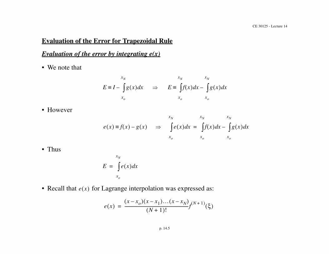
• Trapezoidal Rule integrates the area of the trapezoid between the two data or interpola-tion points.

• Evaluating the error for trapezoidal rule.

• The error is dependent on the integral of the difference .However integrating the dependent error approximation for the interpolatingfunction does not work out in general since is a function of !

• We must express in terms of a series of terms expanded about in order to

evaluate correctly.

• An alternative strategy is to evaluate

by developing Taylor series expansions for , and .

• We do note that as E

E e x f x g x –=

x

e x xo

E e x xd

xo

x1

=

E f x xx1 xo–

2---------------- fo f1+ –d

xo

x1

=

f x fo f1

x1 xo– h=


p. 14.5

Evaluation of the Error for Trapezoidal Rule

Evaluation of the error by integrating e(x)

• We note that

• However

• Thus

• Recall that for Lagrange interpolation was expressed as:

E I g x xd

xo

xN

– E f x x g x xd

xo

xN

–d

xo

xN

e x f x g x – e x xd

xo

xN

f x x g x xd

xo

xN

–d

xo

xN

=

E e x xd

xo

xN

=

e x

e x x xo– x x1– x xN–

N 1+ !---------------------------------------------------------------f

N 1+ =


p. 14.6

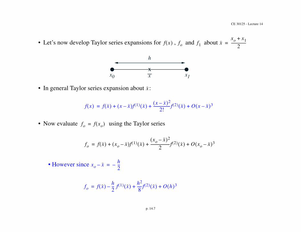
• Notes

• Procedure applies to higher order integration rules as well.

• In general is a function of

• Neglecting the dependence of , can lead to incorrect results. e.g. for Simpson’s

rule you will integrate out the dependent term and the result would be !

• A way you can apply is to take as a series of terms! Then we will

always get the correct answer!

Evaluation of the error for Trapezoidal Rule by Taylor Series expansion

x

x 13--- E 0=

E e x xd

xo

x1

= e x

E Ix1 xo–

2---------------- fo f1+ –=

E f x xo

x1

dxx1 xo–

2---------------- fo f1+ –=


p. 14.7

• Let’s now develop Taylor series expansions for , and about 77

• In general Taylor series expansion about :

• Now evaluate using the Taylor series

• However since

f x fo f1 xxo x1+

2----------------=

xx0 x1

h

x

x

f x f x x x– f 1 x x x– 2

2!------------------ f 2 x O x x– 3+ + +=

fo f xo =

fo f x xo x– f 1 x xo x– 2

2---------------------f 2 x O xo x– 3+ + +=

xo x– h2---–=

fo f x h2--- f 1 x –

h2

8-----f 2 x O h 3+ +=


p. 14.8

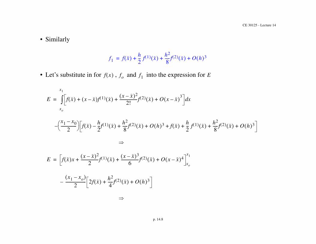
• Similarly

• Let’s substitute in for , and into the expression for

f1 f x h2--- f 1 x h2

8-----f 2 x O h 3+ + +=

f x fo f1 E

E f x x x– f 1 x x x– 22!

------------------f 2 x O x x– 3+ + + xd

xo

x1

=

x1 x0–

2---------------- – f x h

2--- f 1 x –

h2

8-----f 2 x O h 3+ + f x h

2--- f 1 x h2

8-----f 2 x O h 3+ + + +

E f x x x x– 2

2------------------f 1 x x x– 3

6------------------f 2 x O x x– 4+ + +

x1

xo

=

x1 xo–

2--------------------- 2f x h2

4-----f 2 x O h 3+ +–


p. 14.9

• Notes

• Higher order terms have been truncated in this error expression.

• This integration will be exact only for linear.

• However it is third order accurate in

• Error evaluation procedure using T.S. applies to higher order methods as well

E f x x1 xo– x1 x– 2

2---------------------f 1 x

xo x– 2

2---------------------f 1 x –+=

x1 x– 3

6---------------------f 2 x

xo x– 3

6---------------------f 2 x O x1 x– 4 O xo x– 4+ +–+

x1 xo– – f x x1 xo–

8---------------------h2f 2 x –

x1 xo– 2

---------------------O h 3+

Eh2

8----- f 1 x h2

8-----f 1 x –

h3

48------f 2 x h3

48------f 2 x O h 4 h3

8-----f 2 x O h 4+–+ + +=

E h3

12------ f 2 x –=

f x =

h


p. 14.10

Extended Trapezoidal Rule

• Apply trapezoidal rule to multiple “sub-intervals” 78

• Integrate each sub-interval with trapezoidal rule and sum

• Split into equispaced sub-intervals with

• Compute I as:

a

f0f1 f2

x0 x1 x2

fi

fN

bxNxi

x

f(x)

a b N hb a–

N------------=

I f x xd

a

b

f x xd

xi

xi 1+

i 0=

N 1–

= =


p. 14.11

where

.

.

.

• Thus extended trapezoidal rule can be expressed as:

where

Ix1 xo–

2---------------- fo f1+

x2 x1–

2---------------- f1 f2+

xN xN 1––

2------------------------ fN 1– fN+ E a b ++ ++=

Ih2--- f0 2f1 2f2 2fN 1– fN+ + + + + E a b +=

fo f a =

f1 f a h+ =

f2 f a 2h+ =

fi f a ih+ =

Ih2--- f a f b 2 f a ih+

i 1=

N 1–

+ += Nb a–

h------------=


p. 14.12

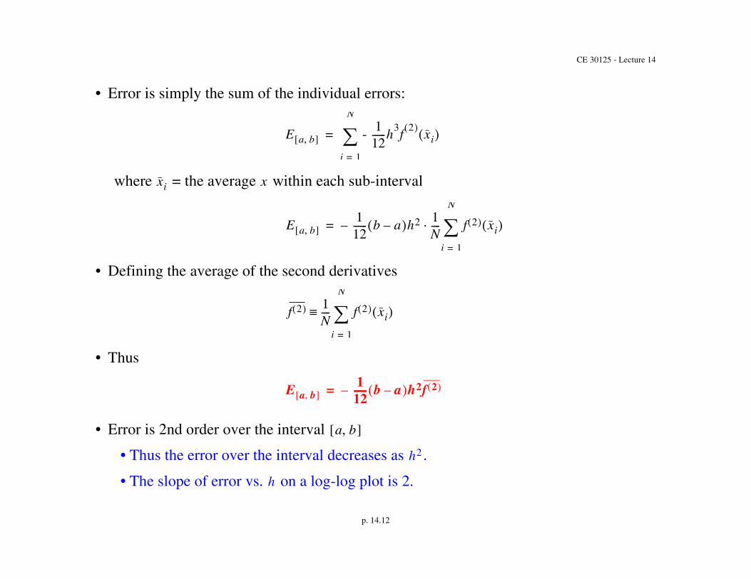
• Error is simply the sum of the individual errors:

where = the average within each sub-interval

• Defining the average of the second derivatives

• Thus

• Error is 2nd order over the interval

• Thus the error over the interval decreases as .

• The slope of error vs. on a log-log plot is 2.

E a b - 1

12------h

3f

2 xi

i 1=

N

=

xi x

E a b 112------– b a– h2 1

N---- f 2 xi

i 1=

N

=

f 2 1N---- f 2 xi

i 1=

N

E a b 112------ b a– h2f 2 –=

a b

h2

h


p. 14.13

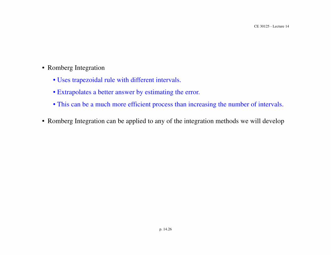
Romberg Integration

• Uses extended trapezoidal rule with two or more different integration point to integra-tion point spacings (in this case equal to the sub-interval spacing), , in conjunctionwith the general form of the error in order to compute one or more terms in the serieswhich represents the error.

• This will then result in a higher order estimate of the integrand.

• More importantly, it will allow us to easily derive an error estimate for the numericalintegrations based on the results using the different grid spacings.

• Consider

where

the exact integrand,

the approximate integral with integration point to integration point spacing

the associated error.

h

I Ih E a b h–+=

I

Ih h

E a b h–

Ihh2--- f a f b 2 f a ih+

i 1=

b a–h

------------ 1–

+ +


p. 14.14

• In general the form of the error term if we had worked out more terms in the error series.

• Notes

• The coefficient

• In general, C, D, E etc. are functions of the average of the various derivatives of over the interval of interest.

• These coefficients are not dependent on the spacing .

• Also we do not worry about the exact form of these coefficients.

• As far as we are concerned, they are unknown constant coefficients over the interval.

E a b h– Ch2 Dh4 Eh6 O h 8+ + +=

C 1

12------ b a– f 2 –=

f

h

a b


p. 14.15

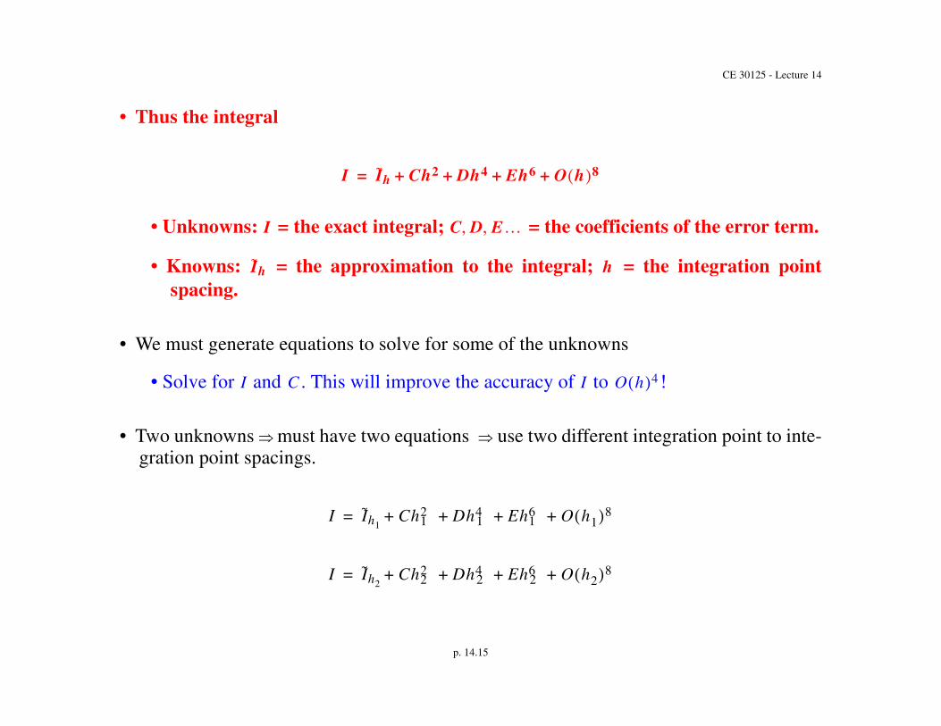
• Thus the integral

• Unknowns: = the exact integral; = the coefficients of the error term.

• Knowns: = the approximation to the integral; = the integration pointspacing.

• We must generate equations to solve for some of the unknowns

• Solve for and . This will improve the accuracy of to !

• Two unknowns must have two equations use two different integration point to inte-gration point spacings.

I Ih Ch2 Dh4 Eh6 O h 8+ + + +=

I C D E

Ih h

I C I O h 4

I Ih1Ch2

1 Dh41 Eh6

1 O h1 8+ + + +=

I Ih2Ch2

2 Dh42 Eh6

2 O h2 8+ + + +=


p. 14.16

• We now have two equations and can therefore solve for 2 unknowns.

• = the exact integral is unknown: = the leading coefficient of the error term isunknown.

• We can solve for and .

• We can not solve for , , ... and the other coefficients since we do not have enoughequations!

• We must select and such that is divided into an integer number of sub-inter-vals. Let

• We compute the approximation to the integral twice.

I C

I C

D E

h1 h2 a b

h1 2h*=

h2 h* base interval = =

2h* I2h*

h* Ih*


p. 14.17

• Thus

• Two equations and 2 unknowns. Thus we can solve for both and .

• Therefore if you have 2 second order accurate approximations to

You can extrapolate a 4th order accurate approximation using the above formula.

I I2h*4Ch2

* 16Dh4* 64Eh6

* O h*

8+ + + +=

I Ih*Ch2

*Dh4

*Eh6

*O h

* 8+ + + +=

I C

I– I2h*– 4Ch2

*16Dh4

*–– 64Eh6

*– O h

* 8+=

4I 4 Ih*4Ch2

* 4Dh4* 4Eh6

* O h*

8+ + + +=

I4 Ih*

I2h*–

3------------------------- 4Dh4

* 20Eh6*–– O h

* 8+=

I

Ih* using h*

I2h* using 2h*


p. 14.18

• More importantly, we can estimate the errors for both the coarse and the fine integrationpoint solutions simply by solving for using the 2 simultaneous equations

• Thus the estimated error associated with the coarse integration point spacing solution,using the coarse and fine integration point spacing solutions is,

• The estimated error associated with the fine integration point spacing solution, using thecoarse and fine integration point spacing solutions is,

C

CIh*

I2h*–

3h*

2--------------------- 5Dh

*

2– O h

* 4+=

2h* h*

E a b 2h*–43--- Ih*

I2h*– O h

* 4+=

2h* h*

E a b h*–13--- Ih*

I2h*– O h

* 4+=


p. 14.19

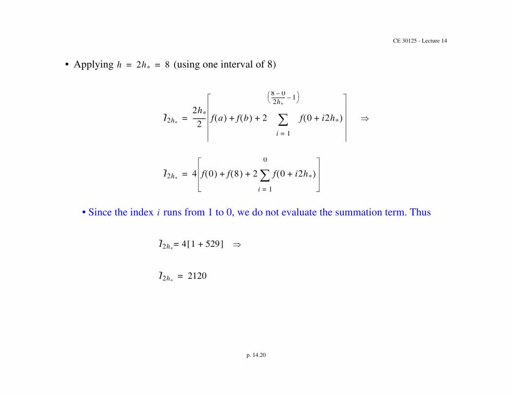
Example

• Consider:

• Integrating exactly

• Let’s integrate numerically

• Apply extended trapezoidal rule using:

• (using one interval of 8)

• (using two intervals of 4)

• Apply the Romberg integration rule we derived when two integral estimates wereobtained using intervals 2h* and h* to obtain a fourth order estimate for the integral

• Estimate the errors associated with the extended trapezoidal rule results

I5x4

8-------- 4x3– 2x 1+ + xd

0

8

=

I 72=

f x 5x4

8-------- 4x3– 2x 1+ += a 0= b 8=

h 2h* 8= =

h h* 4= =


p. 14.20

• Applying (using one interval of 8)

• Since the index runs from 1 to 0, we do not evaluate the summation term. Thus

h 2h* 8= =

I2h*

2h*

2-------- f a f b 2 f 0 i2h*+

i 1=

8 0–2h*

------------ 1–

+ +=

I2h*4 f 0 f 8 2 f 0 i2h*+

i 1=

0

+ +=

i

I2h*= 4 1 529+

I2h*2120=


p. 14.21

• Applying (using two intervals of 4)

h h* 4= =

Ih*

h*

2----- f a f b 2 f a ih+

i 1=

8 0–h*

------------ 1–

+ +=

Ih*2 f 0 f 8 2 f 0 4i+

i 1=

1

+ +=

Ih*2 f 0 f 8 2f 4 + + =

Ih*2 1 529 2 87+ + =

Ih*712=


p. 14.22

• We can obtain an accurate answer using the trapezoidal rule results,

and

• We can also estimate the error associated with the two trapezoidal rule results,

and

• Let’s estimate the error for the trapezoidal rule result with

• Note that the actual error for the trapezoidal rule results with

O h* 4 O h* 2 I2h*

Ih*

I4 Ih*

I2h*–

3------------------------ O h* 4+=

I4 712 2120–

3------------------------------------ O h* 4+=

I 242.6667 O h* 4+=

O h* 2

I2h*Ih*

h 2h* 8= =

E a b 2h*– estimated–43--- Ih*

I2h*– O h

* 4+

43--- 712 2120– 1877.33–= = =

h 2h* 8= =


p. 14.23

• Let’s estimate the error for the trapezoidal rule results with

• Note that the actual error for the trapezoidal rule results with equals

Romberg Integration Using 3 Estimates of the Integral

• Let’s consider using three estimates on

E a b 2h*– actual– I I2h*– 72 2120– 2048.–= = =

h h* 4= =

E a b h*– estimated–13--- Ih*

I2h*– O h

* 4+

13--- 712 2120– 469.33–= = =

h h* 4= =

E a b h*– actual– I Ih*– 72 712– 640.–= = =

I

I Ih1Ch2

1 Dh41 Eh6

1 O h1 8+ + + +=

I Ih2Ch2

2 Dh42 Eh6

2 O h2 8+ + + +=


p. 14.24

• Three equations we can solve for three unknowns: Solve for = exact integral and and = coefficients of the first two terms in the error series!

• Therefore we can now derive an accurate approximation to

• Apply integration point spacings: , and .

• Estimates of the integral are related to the exact integral, I, as:

• We can solve for the unknowns , and !

I Ih3Ch2

3 Dh43 Eh6

3 O h3 8+ + + +=

I CD

O h 6 I

h1 2h*= h2 h*= h3

h*

2-----=

I I2h*4Ch2

* 16Dh4* 64Eh6

* O h* 8+ + + +=

I Ih*Ch2

* Dh4* Eh6

* O h* 8+ + + +=

I Ih*2-----

C4----h2

*D16------h4

*E64------h6

* O h* 8+ + + +=

I C D


p. 14.25

SUMMARY OF LECTURE 14

• Trapezoidal rule is simply applying linear interpolation between two points and inte-grating the approximating polynomial.

• Error for Trapezoidal Rule

• The error can be determined by computing if is expressed in series

form.

• The error can also be determined by Taylor series expansions of the integrationformula and the exact integral.

• Extended trapezoidal rule applies piecewise linear approximations and sums up indi-vidual integrals.

• Error for extended trapezoidal rule is obtained simply by adding errors over all sub-intervals

I145------ 64 Ih*

2-----

20 Ih*I2h*

+– E h* 6 O h* 8+ +=

e x xd

xo

x1

e x


p. 14.26

• Romberg Integration

• Uses trapezoidal rule with different intervals.

• Extrapolates a better answer by estimating the error.

• This can be a much more efficient process than increasing the number of intervals.

• Romberg Integration can be applied to any of the integration methods we will develop

lecture 14 numerical integrationcoast/jjwteach/www/www/30125/pdfnotes/lecture14... · ce 30125 -...

Documents