1

Lecture 14:Predictive and Transform

Coding

Thinh NguyenOregon State University

2

OutlinePCM (Pulse Code Modulation)DPCM (Differential Pulse Code Modulation)Transform codingJPEG

3

Digital Signal RepresentationLoss from A/D conversion

Aliasing (worse than quantization loss) due to samplingLoss due to quantization

Analog signals

sampling quantization

Digital signals

A/D converterDigital Signal processing

D/A converter

Analog signals

4

Signal representation

For perfect re-construction, sampling rate (Nyquist’sfrequency) needs to be twice the maximum frequency of the signal.

However, in practice, loss still occurs due to quantization.

Finer quantization leads to less error at the expense of increased number of bits to represent signals.

5

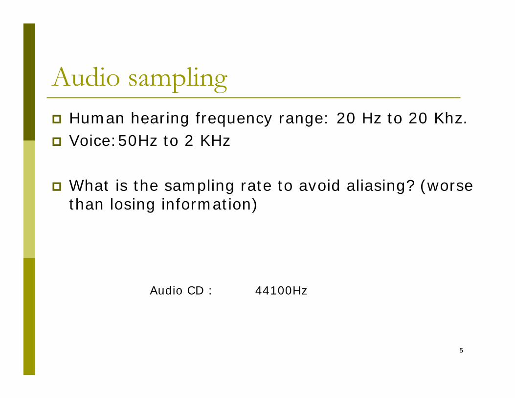
Audio samplingHuman hearing frequency range: 20 Hz to 20 Khz.Voice:50Hz to 2 KHz

What is the sampling rate to avoid aliasing? (worse than losing information)

Audio CD : 44100Hz

6

Audio quantizationSample precision – resolution of signal

Quantization depends on the number of bits used.

Voice quality: 8 bit quantization, 8000 Hz sampling rate. (64 kbps)

CD quality: 16 bit quantization, 44100Hz (705.6 kbps for mono, 1.411 Mbps for stereo).

7

Pulse Code Modulation (PCM)The 2 step process of sampling and quantization is known as Pulse Code Modulation.Used in speech and CD recording.

audio signals

sampling quantizationbits

No compression, unlike MP3

8

DPCM (Differential Pulse Code Modulation)

9

DPCM (Differential Pulse Code Modulation)

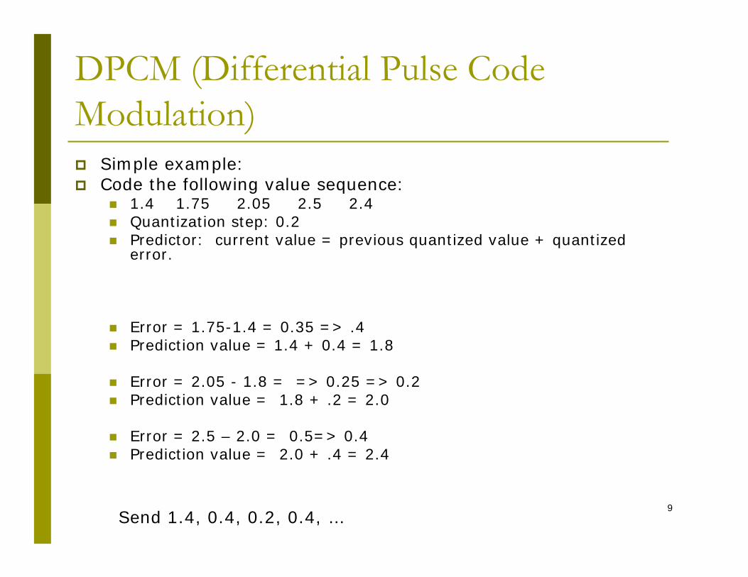
Simple example:Code the following value sequence:

1.4 1.75 2.05 2.5 2.4 Quantization step: 0.2Predictor: current value = previous quantized value + quantizederror.

Error = 1.75-1.4 = 0.35 => .4Prediction value = 1.4 + 0.4 = 1.8

Error = 2.05 - 1.8 = => 0.25 => 0.2Prediction value = 1.8 + .2 = 2.0

Error = 2.5 – 2.0 = 0.5=> 0.4 Prediction value = 2.0 + .4 = 2.4

Send 1.4, 0.4, 0.2, 0.4, …

10

DPCM - Image

0 1/4 1/4

1/2

Linear predictor

11

DPCM - Image

12

Transmission errors in a DPCM systemFor a linear DPCM decoder, the transmission error response is superimposed to the reconstructed signal.

For variable length coding, e.g. Huffman, loss of synchronization due to a single bit error can lead to many prediction error samples.

13

Transmission errors in a DPCM system

Match the following predictors to each images

14

Transmission errors in a DPCM system

15

DPCM-VideoInterframe coding exploits similarity of temporal successive pictures.

Important interframe coding methodsAdaptive intra-interframe codingConditional replenishmentMotion-compensated prediction

16

17

Transform Coding

Why transform Coding?Purpose of transformation is to convert the data into a form where compression is easier.

Transformation yields energy compaction (skewed probability distribution)

Facilitates reduction of irrelevant information.

The transform coefficients can now be quantized according to their statistical properties.

This transformation will reduce the correlation between the pixels.)

18

How Transform Coders Work

Divide the image into 2x1 blocksTypical transforms are 8x8 or 16x16

19

Joint Probability Distribution

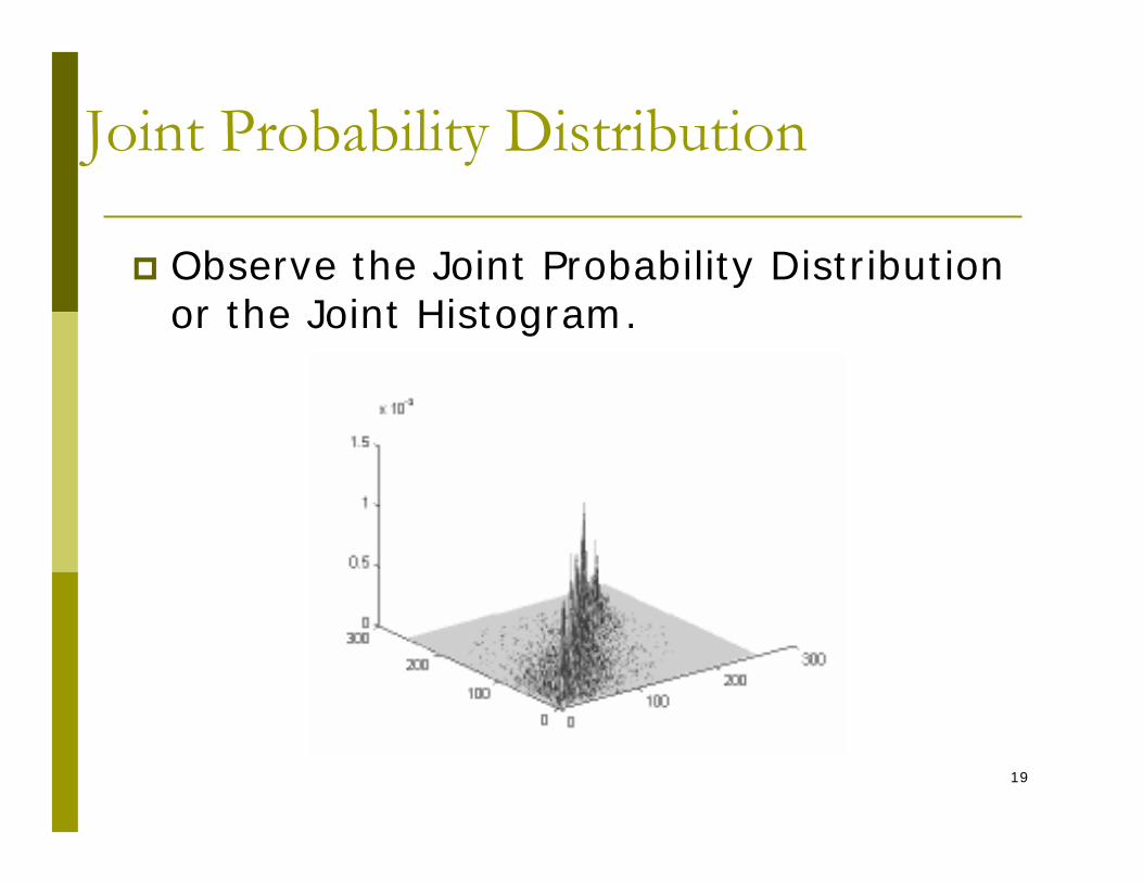
Observe the Joint Probability Distribution or the Joint Histogram.

20

Correlated Pixels

Since adjacent pixels x1 and x2 are highly correlated the joint probability p(x1, x2) is concentrated around the line FF’ and variances are equal because they are the samples of the same image.

21

Pixel Correlation Map

Xave1 =100, Xvar1 =2774Xave2 =100, Xvar2 =2761

x1

x2

22

Rotated Pixels

Rotated 45 degreesY = A X

yave1 =141, yvar1 =5365yave2 =0.13, yvar2= 170

Energy is packed to y1. Can apply entropy coder on y2.

Rotation matrix

y2

y1

45

cos sin 2 2sin cos 2 2

Aθ

θ θθ θ Ο=

⎡ ⎤⎡ ⎤= = ⎢ ⎥⎢ ⎥− −⎣ ⎦ ⎢ ⎥⎣ ⎦

23

Reconstruct the Image

Recover X from Y.Since Y = AX, so

X = A-1Y

Reverse matrix

1

45

cos sin 2 2sin cos 2 2

Aθ

θ θθ θ Ο

−

=

⎡ ⎤− −⎡ ⎤= = ⎢ ⎥⎢ ⎥⎣ ⎦ ⎢ ⎥⎣ ⎦

24

Idea of Transform Coding

Transform the input pixels Y0,Y1,Y2,...,YN-1 into coefficients Y0,Y1,...,YN-1 (real values)

The coefficients are have the property that most of them are near zero. Most of the “energy” is compacted into a few coefficients.

Scalar quantize the coefficientThis is bit allocation.Important coefficients should have more quantization levels.

Entropy encode the quantization symbols

25

Transform Coding Block Diagram

Transmitter or Encoder

Receiver or Decoder

Segment into n*n Blocks

Forward Transform

Quantization and Coder

Original Image f(j,k) F(u,v) F*(uv)

Channel

Combine n*n Blocks

Inverse Transform Decoder

Reconstructed Image f(j,k) F(u,v) F*(uv)

26

Discrete Cosine Transform (DCT)

For conventional image data having reasonably high inter-element correlation.

Avoids the generation of the spurious spectral components which is a problem with DFT and has a fast implementation which avoids complex algebra.

27

Basic Cosine Transform

The basic Cosine Transform is:

where:

28

Inverse Cosine Transform

The inverse cosine transform is:

where:

29

Fast Cosine Transform

2D basis functions of the DCT:

Apply 1D horizontal DCT then 1D vertical DCT

Fast algorithm for scaled 8-DCT

5 multiplications29 additions.

30

Amplitude distribution of the DCTcoefficients

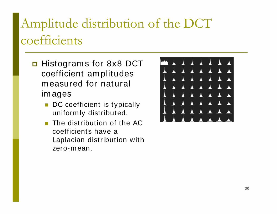
Histograms for 8x8 DCT coefficient amplitudes measured for natural images

DC coefficient is typically uniformly distributed.The distribution of the AC coefficients have a Laplacian distribution with zero-mean.

31

Importance of Coefficients

The DC coefficient is the most important.The AC coefficients become less important as they are farther from the DC coefficient.Example bit allocation table:

32

Karhunen Loève Transform (KLT)

Karhunen Loève Transform (KLT) yields decorrelated transform coefficients.Basis functions are eigenvectors of the covariance matrix of the input signal.KLT achieves optimum energy concentration.Disadvantages:

KLT dependent on signal statisticsKLT not separable for image blocksTransform matrix cannot be factored into sparse matrices

33

Other TransformsWaveletsDFTRemember BWT?

34

JPEGJPEG stands for Joint Photographic Expert GroupA standard image compression method is needed to enable interoperability of equipment from different manufacturerIt is the first international digital image compression standard for continuous-tone images (grayscale or color)

35

“very good” or “excellent” compression rate, reconstructed image quality, transmission ratebe applicable to practically any kind of continuous-tone digital source imagegood complexityhave the following modes of operations:

sequential encodingprogressive encodinglossless encodinghierarchical encoding

JPEG

36

JPEG Encoder Block Diagram

37

JPEG Main operationsQuantization

Different quantization level for different DC and AC coefficients

Zig-zag ScanWhy? -- to group low frequency coefficients in top of vector. Maps 8 x 8 to a 1 x 64 vector

Differential Pulse Code Modulation (DPCM) on DC component

DC component is large and varied, but often close to previous value. Encode the difference from previous 8 x 8 blocks -- DPCM

Run Length Encode (RLE) on AC components1 x 64 vector has lots of zeros in it Keeps skip and value, where skip is the number of zeros and value is the next non-zero component. Send (0,0) as end-of-block sentinel value.

Entropy Coding (Huffman, arithmetic, …) Differential DC and run-length AC values

38

DCT Quantization Table (Luminance)

F'[u, v] = round ( F[u, v] / q[u, v] ).

39

DCT Zig-Zag-Scan

The variances of the DCT transform coefficients are decreasing in a zig-zag manner approximately.

zig-zag-scan + run-level-coding

40

Example

41

JPEG Progressive Model

Why progressive model?Quick transmissionImage built up in a coarse-to-fine passes

First stage: encode a rough but recognizable version of the imageLater stage(s): the image refined by successive scans till get the final imageTwo ways to do this:

Spectral selection – send DC, AC coefficients separatelySuccessive approximation – send the most significant bits first and then the least significant bits

42

JPEG Lossless Model

DPCMSample values Descriptors

Differential pulse code modulation

C BA X

selection value prediction strategy

7

0123

(A+B)/2

no predictionABC

Predictors for lossless coding

B+(A-C)/2

A+B-CA+(B-C)/2

456

43

JPEG Hierarchical Model

Hierarchical model is an alternative of progressive model (pyramid)Steps:

filter and down-sample the original images by the desired number of multiplies of 2 in each dimensionEncode the reduced-size image using one of the above coding modelUse the up-sampled image as a prediction of the origin at this resolution, encode the differenceRepeat till the full resolution image has been encode

44

JPEG-2000JPEG 2000 is the upcoming standard for Still Pictures

Major change from the current JPEG is that wavelets will replace DCT as the means of transform coding.

Among many things it will address: Low bit-rate compression performance, Lossless and lossy compression in a single codestream, Transmission in noisy environment where bit-error is high, Application to both gray/color images and bi-level (text) imagery, natural imagery and computer generated imagery, Interface with MPEG-4, Content-based description.