lecture 16 deep neural generative models - cmsc 35246...
TRANSCRIPT

Lecture 16Deep Neural Generative Models
CMSC 35246: Deep Learning
Shubhendu Trivedi&
Risi Kondor
University of Chicago
May 22, 2017
Lecture 16 Deep Neural Generative Models CMSC 35246

Approach so far:
We have considered simple models and then constructed theirdeep, non-linear variants
Example: PCA (and Linear Autoencoder) to Nonlinear-PCA(Non-linear (deep?) autoencoders)
Example: Sparse Coding (Sparse Autoencoder with lineardecoding) to Deep Sparse Autoencoders
All the models we have considered so far are completelydeterministic
The encoder and decoders have no stochasticity
We don’t construct a probabilistic model of the data
Can’t sample from the model
Lecture 16 Deep Neural Generative Models CMSC 35246

Representations
Figure: Ruslan Salakhutdinov
Lecture 16 Deep Neural Generative Models CMSC 35246

To motivate Deep Neural Generative models, like before, let’sseek inspiration from simple linear models first
Lecture 16 Deep Neural Generative Models CMSC 35246

Linear Factor Model
We want to build a probabilistic model of the input P̃ (x)
Like before, we are interested in latent factors h that explain x
We then care about the marginal:
P̃ (x) = EhP̃ (x|h)
h is a representation of the data
Lecture 16 Deep Neural Generative Models CMSC 35246

Linear Factor Model
The latent factors h are an encoding of the data
Simplest decoding model: Get x after a linear transformationof x with some noise
Formally: Suppose we sample the latent factors from adistribution h ∼ P (h)
Then: x = Wh + b + ε
Lecture 16 Deep Neural Generative Models CMSC 35246

Linear Factor Model
P (h) is a factorial distribution
x1 x2 x3 x4 x5
h1 h2 h3
x = Wh + b + ε
How do learn in such a model?
Let’s look at a simple example
Lecture 16 Deep Neural Generative Models CMSC 35246

Probabilistic PCA
Suppose underlying latent factor has a Gaussian distribution
h ∼ N (h; 0, I)
For the noise model: Assume ε ∼ N (0, σ2I)
Then:P (x|h) = N (x|Wh + b, σ2I)
We care about the marginal P (x) (predictive distribution):
P (x) = N (x|b,WW T + σ2I)
Lecture 16 Deep Neural Generative Models CMSC 35246

Probabilistic PCA
P (x) = N (x|b,WW T + σ2I)
How do we learn the parameters? (EM, ML Estimation)
Let’s look at the ML Estimation:
Let C = WW T + σ2I
We want to maximize `(θ;X) =∑
i logP (xi|θ)
Lecture 16 Deep Neural Generative Models CMSC 35246

Probabilistic PCA: ML Estimation
`(θ;X) =∑i
logP (xi|θ)
= −N2
log |C| − 1
2
∑i
(xi − b)C−1(xi − b)T
= −N2
log |C| − 1
2Tr[(C−1
∑i
xi − b)(xi − b)T ]
=N
2log |C| − 1
2Tr[(C−1S]
Now fit the parameters θ = W,b, σ to maximize log-likelihood
Can also use EM
Lecture 16 Deep Neural Generative Models CMSC 35246

Factor Analysis
Fix the latent factor prior to be the unit Gaussian as before:
h ∼ N (h; 0, I)
Noise is sampled from a Gaussian with a diagonal covariance:
Ψ = diag([σ21, σ22, . . . , σ
2d])
Still consider linear relationship between inputs and observedvariables: Marginal P (x) ∼ N (x; b,WW T + Ψ)
Lecture 16 Deep Neural Generative Models CMSC 35246
Factor Analysis
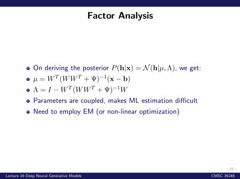
On deriving the posterior P (h|x) = N (h|µ,Λ), we get:
µ = W T (WW T + Ψ)−1(x− b)
Λ = I −W T (WW T + Ψ)−1W
Parameters are coupled, makes ML estimation difficult
Need to employ EM (or non-linear optimization)
Lecture 16 Deep Neural Generative Models CMSC 35246
More General Models
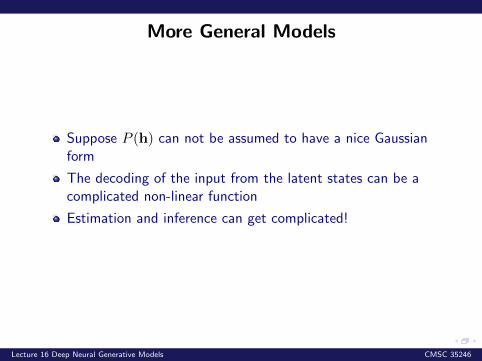
Suppose P (h) can not be assumed to have a nice Gaussianform
The decoding of the input from the latent states can be acomplicated non-linear function
Estimation and inference can get complicated!
Lecture 16 Deep Neural Generative Models CMSC 35246

Earlier we had:
x1 x2 x3 x4 x5
h1 h2 h3
Lecture 16 Deep Neural Generative Models CMSC 35246

Quick Review
Generative models can be modeled as directed graphicalmodels
The nodes represent random variables and arcs indicatedependency
Some of the random variables are observed, others are hidden
Lecture 16 Deep Neural Generative Models CMSC 35246

Sigmoid Belief Networks
. . .x
. . .h1
. . .h2
. . .h3
Just like a feedfoward network, but with arrows reversed.
Lecture 16 Deep Neural Generative Models CMSC 35246

Sigmoid Belief Networks
Let x = h0. Consider binary activations, then:
P (hki = 1|hk+1) = sigm(bki +∑j
W k+1i,j hk+1
j )
The joint probability factorizes as:
P (x,h1, . . . ,hl) = P (hl)( l−1∏k=1
P (hk|hk+1))P (x|h1)
Marginalization yields P (x), intractable in practice except forvery small models
Lecture 16 Deep Neural Generative Models CMSC 35246
Sigmoid Belief Networks
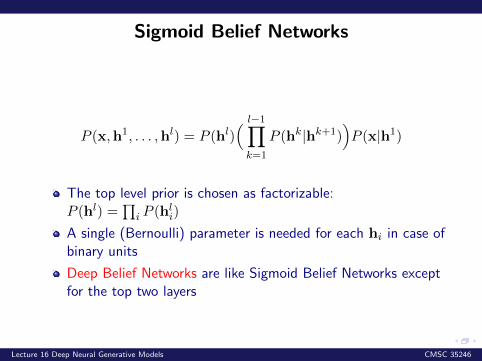
P (x,h1, . . . ,hl) = P (hl)( l−1∏k=1
P (hk|hk+1))P (x|h1)
The top level prior is chosen as factorizable:P (hl) =
∏i P (hli)
A single (Bernoulli) parameter is needed for each hi in case ofbinary units
Deep Belief Networks are like Sigmoid Belief Networks exceptfor the top two layers
Lecture 16 Deep Neural Generative Models CMSC 35246

Sigmoid Belief Networks
General case models are called Helmholtz Machines
Two key references:
• G. E. Hinton, P. Dayan, B. J. Frey, R. M. Neal: TheWake-Sleep Algorithm for Unsupervised Neural Networks,In Science, 1995
• R. M. Neal: Connectionist Learning of Belief Networks,In Artificial Intelligence, 1992
Lecture 16 Deep Neural Generative Models CMSC 35246

Deep Belief Networks
. . .x
. . .h1
. . .h2
. . .h3
The top two layers now have undirected edges
Lecture 16 Deep Neural Generative Models CMSC 35246

Deep Belief Networks
The joint probability changes as:
P (x,h1, . . . ,hl) = P (hl,hl−1)( l−2∏k=1
P (hk|hk+1))P (x|h1)
Lecture 16 Deep Neural Generative Models CMSC 35246

Deep Belief Networks
. . .hl
. . .hl+1
The top two layers are a Restricted Boltzmann Machine
A RBM has the joint distribution:
P (hl+1,hl) ∝ exp(b′hl−1 + c′hl + hlWhl−1)
We will return to RBMs and training procedures in a while,but first we look at the mathematical machinery that willmake our task easier
Lecture 16 Deep Neural Generative Models CMSC 35246
Energy Based Models
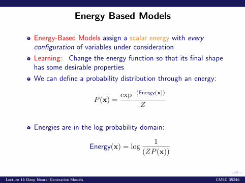
Energy-Based Models assign a scalar energy with everyconfiguration of variables under consideration
Learning: Change the energy function so that its final shapehas some desirable properties
We can define a probability distribution through an energy:
P (x) =exp−(Energy(x))
Z
Energies are in the log-probability domain:
Energy(x) = log1
(ZP (x))
Lecture 16 Deep Neural Generative Models CMSC 35246

Energy Based Models
P (x) =exp−(Energy(x))
Z
Z is a normalizing factor called the Partition Function
Z =∑x
exp(−Energy(x))
How do we specify the energy function?
Lecture 16 Deep Neural Generative Models CMSC 35246
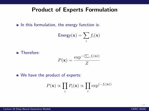
Product of Experts Formulation
In this formulation, the energy function is:
Energy(x) =∑i
fi(x)
Therefore:
P (x) =exp−(
∑i fi(x))
Z
We have the product of experts:
P (x) ∝∏i
Pi(x) ∝∏i
exp(−fi(x))
Lecture 16 Deep Neural Generative Models CMSC 35246

Product of Experts Formulation
P (x) ∝∏i
Pi(x) ∝∏i
exp(−fi(x))
Every expert fi can be seen as enforcing a constraint on x
If fi is large =⇒ Pi(x) is small i.e. the expert thinks x isimplausible (constraint violated)
If fi is small =⇒ Pi(x) is large i.e. the expert thinks x isplausible (constraint satisfied)
Contrast this with mixture models
Lecture 16 Deep Neural Generative Models CMSC 35246

Latent Variables
x is observed, let’s say h are hidden factors that explain x
The probability then becomes:
P (x,h) =exp−(Energy(x,h))
Z
We only care about the marginal:
P (x) =∑h
exp−(Energy(x,h))
Z
Lecture 16 Deep Neural Generative Models CMSC 35246

Latent Variables
P (x) =∑h
exp−(Energy(x,h))
Z
We introduce another term in analogy from statistical physics:free energy:
P (x) =exp−(FreeEnergy(x))
Z
Free Energy is just a marginalization of energies in thelog-domain:
FreeEnergy(x) = − log∑h
exp−(Energy(x,h))
Lecture 16 Deep Neural Generative Models CMSC 35246

Latent Variables
P (x) =exp−(FreeEnergy(x))
Z
Likewise, the partition function:
Z =∑x
exp−FreeEnergy(x)
We have an expression for P (x) (and hence for the datalog-likelihood). Let us see how the gradient looks like
Lecture 16 Deep Neural Generative Models CMSC 35246

Data Log-Likelihood Gradient
P (x) =exp−(FreeEnergy(x))
Z
The gradient is simply working from the above:
∂ logP (x)
∂θ= −∂FreeEnergy(x)
∂θ
+1
Z
∑x̃
exp−(FreeEnergy(x̃))∂FreeEnergy(x̃)
∂θ
Note that P (x̃) = exp−(FreeEnergy(x̃))
Lecture 16 Deep Neural Generative Models CMSC 35246

Data Log-Likelihood Gradient
The expected log-likelihood gradient over the training set hasthe following form:
EP̃
[∂ logP (x)
∂θ
]= EP̃
[∂FreeEnergy(x)
∂θ
]+EP
[∂FreeEnergy(x)
∂θ
]
Lecture 16 Deep Neural Generative Models CMSC 35246

Data Log-Likelihood Gradient
EP̃
[∂ logP (x)
∂θ
]= EP̃
[∂FreeEnergy(x)
∂θ
]+EP
[∂FreeEnergy(x)
∂θ
]
P̃ is the empirical training distribution
Easy to compute!
Lecture 16 Deep Neural Generative Models CMSC 35246

Data Log-Likelihood Gradient
EP̃
[∂ logP (x)
∂θ
]= EP̃
[∂FreeEnergy(x)
∂θ
]+EP
[∂FreeEnergy(x)
∂θ
]
P is the model distribution (exponentially manyconfigurations!)
Usually very hard to compute!
Resort to Markov Chain Monte Carlo to get a stochasticestimator of the gradient
Lecture 16 Deep Neural Generative Models CMSC 35246

A Special Case
Suppose the energy has the following form:
Energy(x,h) = −β(x) +∑i
γi(x,hi)
The free energy, and numerator of log likelihood can becomputed tractably!
What is P (x)?
What is the FreeEnergy(x)?
Lecture 16 Deep Neural Generative Models CMSC 35246
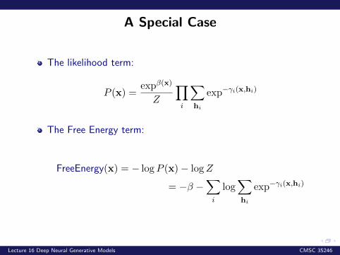
A Special Case
The likelihood term:
P (x) =expβ(x)
Z
∏i
∑hi
exp−γi(x,hi)
The Free Energy term:
FreeEnergy(x) = − logP (x)− logZ
= −β −∑i
log∑hi
exp−γi(x,hi)
Lecture 16 Deep Neural Generative Models CMSC 35246

Restricted Boltzmann Machines
. . .hl
. . .hl+1
Recall the form of energy:
Energy(x,h) = −bTx− cTh− hTWx
Takes the earlier nice form with β(x) = bTx andγi(x,hi) = hi(ci +Wix)
Originally proposed by Smolensky (1987) who called themHarmoniums as a special case of Boltzmann Machines
Lecture 16 Deep Neural Generative Models CMSC 35246

Restricted Boltzmann Machines
. . .hl
. . .hl+1
As seen before, the Free Energy can be computed efficiently:
FreeEnergy(x) = −bTx−∑i
log∑hi
exphi(ci+Wix)
The conditional probability:
P (h|x) =exp (bTx + cTh + hTWx)∑h̃ exp (bTx + cT h̃ + h̃TWx)
=∏i
P (hi|x)
Lecture 16 Deep Neural Generative Models CMSC 35246

Restricted Boltzmann Machines
. . .hl
. . .hl+1
x and h play symmetric roles:
P (x|h) =∏i
P (xi|h)
The common transfer (for the binary case):
P (hi = 1|x) = σ(ci +Wix)
P (xj = 1|h) = σ(bj +W T:,jh)
Lecture 16 Deep Neural Generative Models CMSC 35246

Approximate Learning and Gibbs Sampling
EP̃
[∂ logP (x)
∂θ
]= EP̃
[∂FreeEnergy(x)
∂θ
]+EP
[∂FreeEnergy(x)
∂θ
]
We saw the expression for Free Energy for a RBM. But thesecond term was intractable. How do learn in this case?
Replace the average over all possible input configurations bysamples
Run Markov Chain Monte Carlo (Gibbs Sampling):
First sample x1 ∼ P̃ (x), then h1 ∼ P (h|x1), thenx2 ∼ P (x|h1), then h2 ∼ P (h|x2) till xk+1
Lecture 16 Deep Neural Generative Models CMSC 35246

Approximate Learning, Alternating GibbsSampling
We have already seen: P (x|h) =∏i
P (xi|h) and
P (h|x) =∏i
P (hi|x)
With: P (hi = 1|x) = σ(ci +Wix) andP (xj = 1|h) = σ(bj +W T
:,jh)
Lecture 16 Deep Neural Generative Models CMSC 35246

Training a RBM: The Contrastive DivergenceAlgorithm
Start with a training example on the visible units
Update all the hidden units in parallel
Update all the visible units in parallel to obtain areconstruction
Update all the hidden units again
Update model parameters
Aside: Easy to extend RBM (and contrastive divergence) tothe continuous case
Lecture 16 Deep Neural Generative Models CMSC 35246

Boltzmann Machines
A model in which the energy has the form:
Energy(x,h) = −bTx− cTh− hTWx− xTUx− hTV h
Originally proposed by Hinton and Sejnowski (1983)
Important historically. But very difficult to train (why?)
Lecture 16 Deep Neural Generative Models CMSC 35246

Back to Deep Belief Networks
. . .x
. . .h1
. . .h2
. . .h3
P (x,h1, . . . ,hl) = P (hl,hl−1)( l−2∏k=1
P (hk|hk+1))P (x|h1)
Lecture 16 Deep Neural Generative Models CMSC 35246

Greedy Layer-wise Training of DBNs
Reference: G. E. Hinton, S. Osindero and Y-W Teh: A FastLearning Algorithm for Deep Belief Networks, In NeuralComputation, 2006.
First Step: Construct a RBM with input x and a hidden layerh, train the RBM
Stack another layer on top of the RBM to form a new RBM.Fix W 1, sample from P (h1|x), train W 2 as RBM
Continue till k layers
Implicitly defines P (x) and P (h) (variational bound justifieslayerwise training)
Can then be discriminatively fine-tuned using backpropagation
Lecture 16 Deep Neural Generative Models CMSC 35246
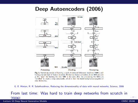
Deep Autoencoders (2006)
G. E. Hinton, R. R. Salakhutdinov, Reducing the dimensionality of data with neural networks, Science, 2006
From last time: Was hard to train deep networks from scratch in2006!
Lecture 16 Deep Neural Generative Models CMSC 35246

Semantic Hashing
G. Hinton and R. Salakhutdinov, ”Semantic Hashing”, 2006
Lecture 16 Deep Neural Generative Models CMSC 35246

Why does Unsupervised Pre-training work?
Regularization. Feature representations that are good forP (x) are good for P (y|x)
Optimization: Unsupervised pre-training leads to betterregions of the space i.e. better than random initialization
Lecture 16 Deep Neural Generative Models CMSC 35246
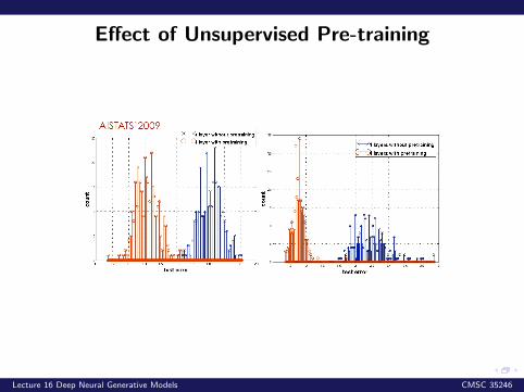
Effect of Unsupervised Pre-training
Lecture 16 Deep Neural Generative Models CMSC 35246

Effect of Unsupervised Pre-training
Lecture 16 Deep Neural Generative Models CMSC 35246

Important topics we didn’t talk about in detail/at all:
• Joint unsupervised training of all layers (Wake-Sleepalgorithm)
• Deep Boltzmann Machines• Variational bounds justifying greedy layerwise training• Conditional RBMs, Multimodal RBMs, Temporal RBMs
etc
Lecture 16 Deep Neural Generative Models CMSC 35246

Next Time
Some Applications of methods we just considered
Generative Adversarial Networks
Lecture 16 Deep Neural Generative Models CMSC 35246