lecture 17: chapter 7, section 3 continuous random
TRANSCRIPT

©2011 Brooks/Cole, CengageLearning
Elementary Statistics: Looking at the Big Picture 1
Lecture 17: Chapter 7, Section 3Continuous Random Variables;Normal DistributionRelevance of Normal DistributionContinuous Random Variables68-95-99.7 Rule for Normal R.V.sStandardizing/UnstandardizingProbabilities for Standard/Non-standard Normal R.V.s

©2011 Brooks/Cole,Cengage Learning
Elementary Statistics: Looking at the Big Picture L17.2
Looking Back: Review
4 Stages of Statistics Data Production (discussed in Lectures 1-4) Displaying and Summarizing (Lectures 5-12) Probability
Finding Probabilities (discussed in Lectures 13-14) Random Variables (introduced in Lecture 15)
Binomial (discussed in Lecture 16) Normal
Sampling Distributions
Statistical Inference

©2011 Brooks/Cole,Cengage Learning
Elementary Statistics: Looking at the Big Picture L17.3
Role of Normal Distribution in Inference Goal: Perform inference about unknown
population proportion, based on sampleproportion
Strategy: Determine behavior of sampleproportion in random samples with knownpopulation proportion
Key Result: Sample proportion followsnormal curve for large enough samples.
Looking Ahead: Similar approach will be taken with means.

©2011 Brooks/Cole,Cengage Learning
Elementary Statistics: Looking at the Big Picture L17.4
Discrete vs. Continuous Distributions Binomial Count X
discrete (distinct possible values like numbers1, 2, 3, …)
Sample Proportion also discrete (distinct values like count)
Normal Approx. to Sample Proportion continuous (follows normal curve) Mean p, standard deviation

©2011 Brooks/Cole,Cengage Learning
Elementary Statistics: Looking at the Big Picture L17.5
Sample Proportions Approx. Normal (Review)
Proportion of tails in n=16 coinflips (p=0.5) has
Proportion of lefties (p=0.1) in n=100 people has, shape approx normal
, shape approx normal

©2011 Brooks/Cole,Cengage Learning
Elementary Statistics: Looking at the Big Picture L17.7
Example: Variable Types Background: Variables in survey excerpt:
Question: Identify type (cat, discrete quan, continuous quan) Age? Breakfast? Comp (daily min. on computer)? Credits?
Response: Age: Breakfast: Comp (daily time in min. on computer): Credits:

©2011 Brooks/Cole,Cengage Learning
Elementary Statistics: Looking at the Big Picture L17.8
Probability Histogram for Discrete R.V.Histogram for male shoe size X represents
probability by area of bars P(X ≤ 9) (on left) P(X < 9) (on right)
For discrete R.V., strict inequality or not matters.
©2011 Brooks/Cole,Cengage Learning
Elementary Statistics: Looking at the Big Picture L17.9
Definition
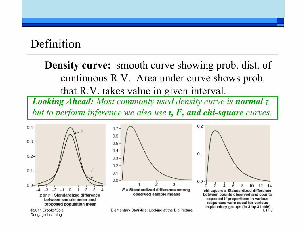
Density curve: smooth curve showing prob. dist. ofcontinuous R.V. Area under curve shows prob.that R.V. takes value in given interval.
Looking Ahead: Most commonly used density curve is normal zbut to perform inference we also use t, F, and chi-square curves.

©2011 Brooks/Cole,Cengage Learning
Elementary Statistics: Looking at the Big Picture L17.11
Density Curve for Continuous R.V.Density curve for male foot length X represents
probability by area under curve.
Continuous RV: strict inequality or not doesn’t matter.A Closer Look: Shoe sizes are discrete; foot lengths are continuous.
©2011 Brooks/Cole,Cengage Learning
Elementary Statistics: Looking at the Big Picture L17.13
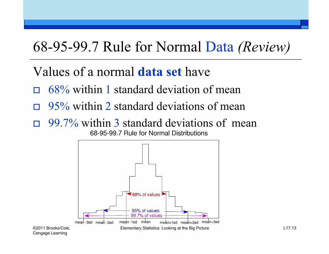
68-95-99.7 Rule for Normal Data (Review)Values of a normal data set have 68% within 1 standard deviation of mean 95% within 2 standard deviations of mean 99.7% within 3 standard deviations of mean

©2011 Brooks/Cole,Cengage Learning
Elementary Statistics: Looking at the Big Picture L17.14
68-95-99.7 Rule: Normal Random VariableSample at random from normal population; for sampled value X
(a R.V.), probability is 68% that X is within 1 standard deviation of mean 95% that X is within 2 standard deviations of mean 99.7% that X is within 3 standard deviations of mean

©2011 Brooks/Cole,Cengage Learning
Elementary Statistics: Looking at the Big Picture L17.15
68-95-99.7 Rule: Normal Random VariableLooking Back: We use Greek letters to denotepopulation mean and standard deviation.

©2011 Brooks/Cole,Cengage Learning
Elementary Statistics: Looking at the Big Picture L17.17
Example: 68-95-99.7 Rule for Normal R.V. Background: IQ for randomly chosen adult is normal R.V.
X with . Question: What does Rule tell us about distribution of X ? Response: We can sketch distribution of X:

©2011 Brooks/Cole,Cengage Learning
Elementary Statistics: Looking at the Big Picture L17.19
Example: Finding Probabilities with Rule
Background: IQ for randomly chosen adult isnormal R.V. X with .
Question: Prob. of IQ between 70 and 130 = ? Response:

©2011 Brooks/Cole,Cengage Learning
Elementary Statistics: Looking at the Big Picture L17.21
Example: Finding Probabilities with Rule
Background: IQ for randomly chosen adult isnormal R.V. X with .
Question: Prob. of IQ less than 70 = ? Response:

©2011 Brooks/Cole,Cengage Learning
Elementary Statistics: Looking at the Big Picture L17.23
Example: Finding Probabilities with Rule
Background: IQ for randomly chosen adult isnormal R.V. X with .
Question: Prob. of IQ less than 100 = ? Response:

©2011 Brooks/Cole,Cengage Learning
Elementary Statistics: Looking at the Big Picture L17.25
Example: Finding Values of X with Rule
Background: IQ for randomly chosen adult isnormal R.V. X with .
Question: Prob. is 0.997 that IQ is between…? Response:

©2011 Brooks/Cole,Cengage Learning
Elementary Statistics: Looking at the Big Picture L17.27
Example: Finding Values of X with Rule
Background: IQ for randomly chosen adult isnormal R.V. X with .
Question: Prob. is 0.025 that IQ is above…? Response:

©2011 Brooks/Cole,Cengage Learning
Elementary Statistics: Looking at the Big Picture L17.29
Example: Using Rule to Evaluate Probabilities
Background: Foot length of randomly chosen adultmale is normal R.V. X with (in.)
Question: How unusual is foot less than 6.5 inches? Response:

©2011 Brooks/Cole,Cengage Learning
Elementary Statistics: Looking at the Big Picture L17.31
Example: Using Rule to Estimate Probabilities
Background: Foot length of randomly chosen adultmale is normal R.V. X with (in.)
Question: How unusual is foot more than 13 inches? Response:

©2011 Brooks/Cole,Cengage Learning
Elementary Statistics: Looking at the Big Picture L17.32
Definition (Review) z-score, or standardized value, tells how
many standard deviations below or above themean the original value is:
Notation for Population: z>0 for x above mean z<0 for x below mean
Unstandardize:

©2011 Brooks/Cole,Cengage Learning
Elementary Statistics: Looking at the Big Picture L17.33
Standardizing Values of Normal R.V.s
Standardizing to z lets us avoid sketching a differentcurve for every normal problem: we can alwaysrefer to same standard normal (z) curve:

©2011 Brooks/Cole,Cengage Learning
Elementary Statistics: Looking at the Big Picture L17.35
Example: Standardized Value of Normal R.V.
Background: Typical nightly hours slept by collegestudents normal;
Question: How many standard deviations below orabove mean is 9 hours?
Response: Standardize to z = _________________(9 is _____ standard deviations above mean)
©2011 Brooks/Cole,Cengage Learning
Elementary Statistics: Looking at the Big Picture L17.37
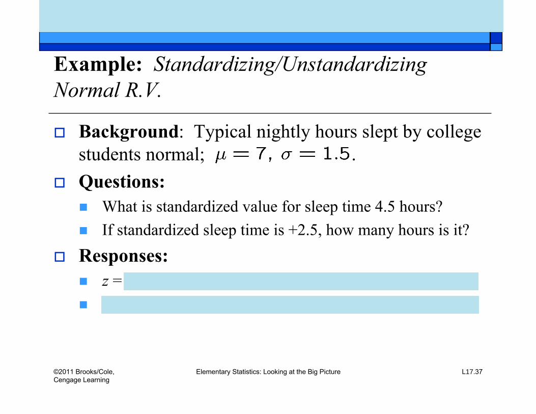
Example: Standardizing/UnstandardizingNormal R.V.
Background: Typical nightly hours slept by collegestudents normal; .
Questions: What is standardized value for sleep time 4.5 hours? If standardized sleep time is +2.5, how many hours is it?
Responses: z = ___________________________________________ ______________________________________________

©2011 Brooks/Cole,Cengage Learning
Elementary Statistics: Looking at the Big Picture L17.38
Interpreting z-scores (Review)
This table classifies ranges of z-scoresinformally, in terms of being unusual or not.
Looking Ahead: Inference conclusions will hinge on whetheror not a standardized score can be considered “unusual”.

©2011 Brooks/Cole,Cengage Learning
Elementary Statistics: Looking at the Big Picture L14.40
Example: Characterizing Normal Values Basedon z-Scores Background: Typical nightly hours slept by college students
normal; . Questions: How unusual is a sleep time of
4.5 hours (z = -1.67)? 10.75 hours (z = +2.5)? Responses:
Sleep time of 4.5 hours (z = -1.67): __________________ Sleep time of 10.75 hours (z = +2.5): ________________

©2011 Brooks/Cole,Cengage Learning
Elementary Statistics: Looking at the Big Picture L17.41
Normal Probability Problems Estimate probability given z
Probability close to 0 or 1 for extreme z Estimate z given probability Estimate probability given non-standard x Estimate non-standard x given probability

©2011 Brooks/Cole,Cengage Learning
Elementary Statistics: Looking at the Big Picture L17.43
Example: Estimating Probability Given z Background: Sketch of 68-95-99.7 Rule for Z
Question: Estimate P(Z<-1.47)? Response:

©2011 Brooks/Cole,Cengage Learning
Elementary Statistics: Looking at the Big Picture L17.45
Example: Estimating Probability Given z Background: Sketch of 68-95-99.7 Rule for Z
Question: Estimate P(Z>+0.75)? Response:
©2011 Brooks/Cole,Cengage Learning
Elementary Statistics: Looking at the Big Picture L17.47
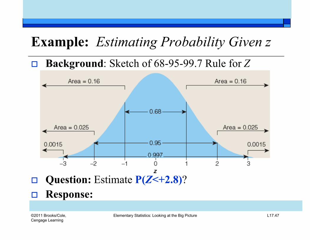
Example: Estimating Probability Given z Background: Sketch of 68-95-99.7 Rule for Z
Question: Estimate P(Z<+2.8)? Response:
©2011 Brooks/Cole,Cengage Learning
Elementary Statistics: Looking at the Big Picture L17.50
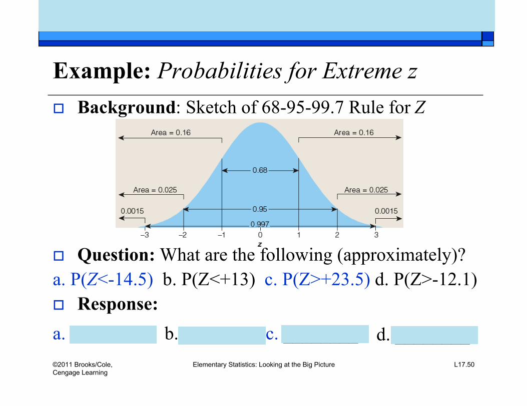
Example: Probabilities for Extreme z Background: Sketch of 68-95-99.7 Rule for Z
Question: What are the following (approximately)?a. P(Z<-14.5) b. P(Z<+13) c. P(Z>+23.5) d. P(Z>-12.1) Response:a. ________ b. _______ c. ________ d. ________

©2011 Brooks/Cole,Cengage Learning
Elementary Statistics: Looking at the Big Picture L17.53
Example: Estimating z Given Probability Background: Sketch of 68-95-99.7 Rule for Z
Question: Prob. is 0.01 that Z < what value? Response:
©2011 Brooks/Cole,Cengage Learning
Elementary Statistics: Looking at the Big Picture L17.55
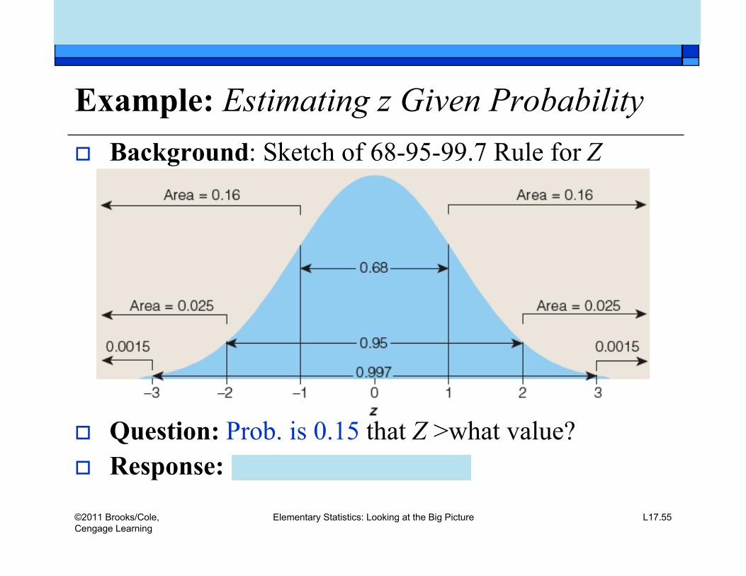
Example: Estimating z Given Probability Background: Sketch of 68-95-99.7 Rule for Z
Question: Prob. is 0.15 that Z >what value? Response:

©2011 Brooks/Cole,Cengage Learning
Elementary Statistics: Looking at the Big Picture L17.58
Example: Estimating Probability Given x Background: Hrs. slept X normal; .
Question: Estimate P(X>9)? Response:

©2011 Brooks/Cole,Cengage Learning
Elementary Statistics: Looking at the Big Picture L17.60
Example: Estimating Probability Given x Background: Hrs. slept X normal; .
Question: Estimate P(6<X<8)? Response:
A Closer Look: -0.67 and +0.67are the quartiles of the z curve.
©2011 Brooks/Cole,Cengage Learning
Elementary Statistics: Looking at the Big Picture L17.63
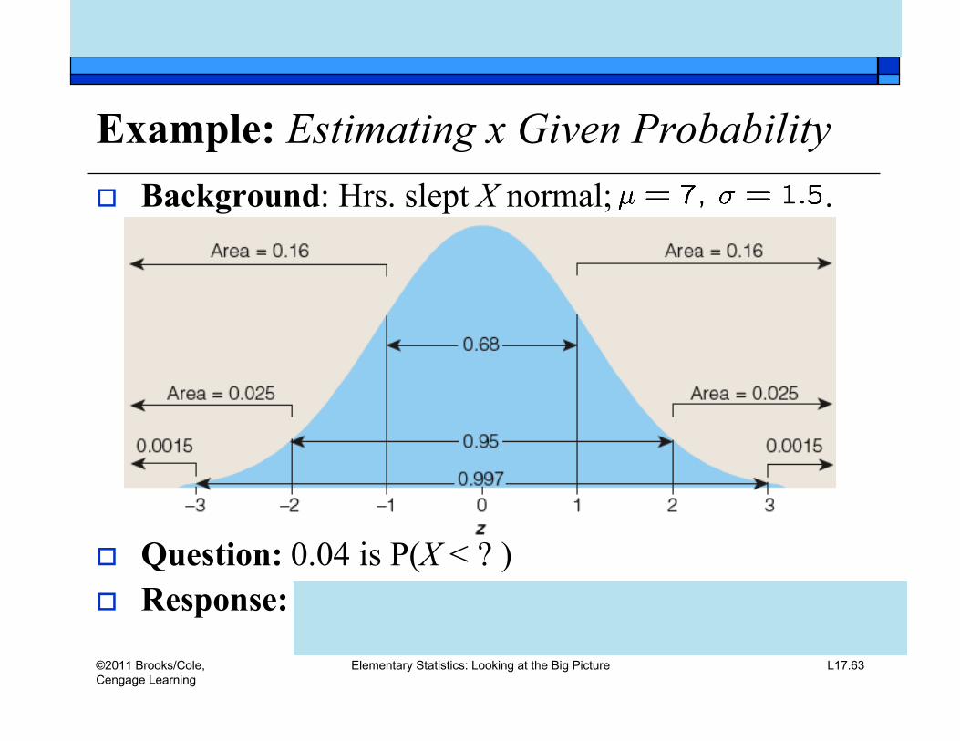
Example: Estimating x Given Probability Background: Hrs. slept X normal; .
Question: 0.04 is P(X < ? ) Response:

©2011 Brooks/Cole,Cengage Learning
Elementary Statistics: Looking at the Big Picture L17.65
Example: Estimating x Given Probability Background: Hrs. slept X normal; .
Question: 0.20 is P(X > ?) Response:

©2011 Brooks/Cole,Cengage Learning
Elementary Statistics: Looking at the Big Picture L17.66
Strategies for Normal Probability Problems Estimate probability given non-standard x
Standardize to z Estimate probability using Rule
Estimate non-standard x given probability Estimate z Unstandardize to x
©2011 Brooks/Cole,Cengage Learning
Elementary Statistics: Looking at the Big Picture L17.67
Lecture Summary(Normal Random Variables)
Relevance of normal distribution Continuous random variables; density curves 68-95-99.7 Rule for normal R.V.s Standardizing/unstandardizing Probability problems
Find probability given z Find z given probability Find probability given x Find x given probability