lecture 18, y23 distribution

8/6/2019 Lecture 18, Y23 distribution

http://slidepdf.com/reader/full/lecture-18-y23-distribution 1/11

Slide 1 of 11

Today’s lecture

Y 23 distribution

Literature:

G. Dissertori, M. Schmelling, Phys. Lett. B 361 (1995) 167-178

A. Banfi, G. Salam, G. Zanderighi, JHEP 01 (2002) 018

A.Heister et al., Eur.Phys.J. C35 (2004) 457

G.Abbiendi at al., Eur. Phys. J. C40 (2005) 287

B. Adeva et al., Z. Phys C55 (1992) 39

|

1|7/25/11



Slide 2 of 11

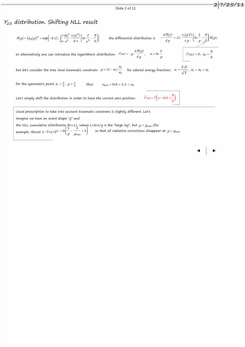
Y 23 distribution. Shifting NLL result

f Hu 0L = 0, u 0 =32

u = ln1 y

f Hu L = - y „ R I y M

„ y ,or alternatively one can introduce the logarithmic distribution:

but let's consider the tree-level kinematic constrain: y = H1 - x 1L x 2

x 3for odered energy fractions: x i =

2 E i

t , x 1 > x 2 > x 3

for the symmetric point x i =23 , y =

13 thus u min = ln3 º 1.1 < u 0

Let's simply shift the distribution in order to have the correct zero position: f èHu L = f u - ln3 +

32

.

Usual prescription to take into account kinematic constrans is slightly different. Let's

imagine we have an event shape "y" andthe NLL cumulative distribution R(a,L), where L=ln1/y is the "large log", but y < y max (for

example, thrust 1-T<1/2), then:

R I y M = ADq I y ME2 = expC-2 C F ‡ yt

t d m2

m2

as I m2M2 p

lnt

m2 -32

G -„ R I M

„ y = C F

as I y t Mp y

ln1 y

-32

R I y M,the differential distribution is

L Ø ln1 y

-1

y max+ 1 so that all radiative corrections disappear at y = y max

|

2|7/25/11



Slide 3 of 11

Y 23 distribution. NLL accuracy

2 4 6 8 10

0.00

0.05

0.10

0.15

0.20

-lnH y 23L

y 2 3

d s ê d y 2 3

BSZ result

CKKW numeric

CKKW analytic

Analytic shifted

as in "Z pole scheme"

|

3|7/25/11



Slide 4 of 11

Y 23 distribution. First nontrivial corrections

2 p

as C F

ds

sH0L dy = -7 + 12 b -

3 y + 16 y -

I1 - y M I12 y - 12 b y - 5 y 2MI2 - 2 b - y M2 +

6 - 8 y + 2 y 2

1 - b + y

+b 2 + 2 b y + 4 y 2

1 - y -

4 y

1 - y LogC1 + y

1 - y G -

1

y

1 + y

1 - y LogC2 - 2 b - y

2 - 2 b + y G

+

2

y LogCy - 1 + b

y + 1 - b G + 2

1 + y

1 - y LogC1 - y

2 G +

2 + y

y LogC21 - y

2 - b G

+6 - 10 y + 8 y 2

1 - y LogC2 2 - 2 b - y

1 - y G -

4 y I1 - y M LogC y

1 - b G

-1 + y

1- y

LogA2 b y - y E + I8 - 4 y MLogC 2 y

1-

b +

y

G,

b = 1 + y

4-

y

2+

y 2

16

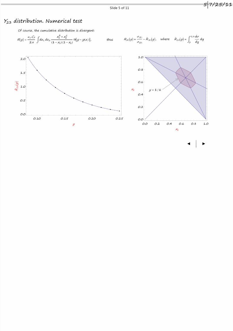
ds

sH0L dy=

as C F

2 p‡ dx1 dx2

x 12

+ x 22

H1 - x 1L H1 - x 2L dI y - y H x i LM, y = H1 - x 1L x 2

x 3for odered energy fractions: x i =

2 E i

t , x 1 > x 2 > x 3

six sectors

|

4|7/25/11

|



Slide 5 of 11

Y 23 distribution. Numerical test

|

5|7/25/11

|



Slide 6 of 11

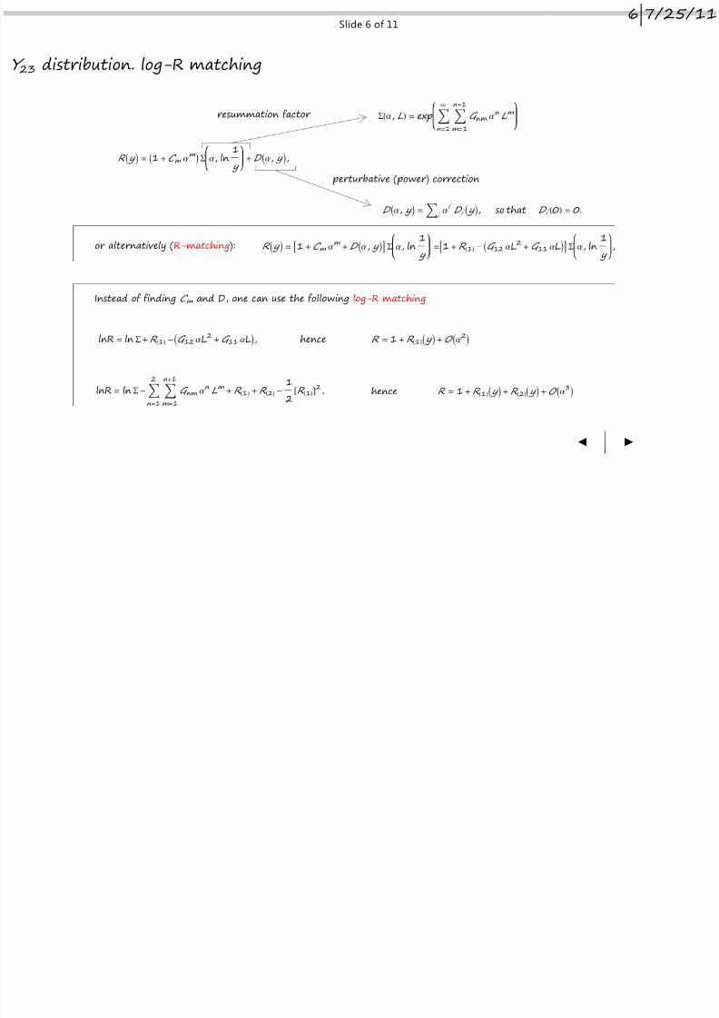
Y 23 distribution. log-R matching

R I y M = I1 + C m am M S a, ln

1 y

+ D Ia, y M,

lnR = ln S + R H1L -IG 12 aL2+ G 11 aLM,

SHa, L L = exp ‚n =1

¶

‚m =1

n +1

G nm an L m

D Ia, y M = ‚i

ai D i I y M, so that D i H0L = 0.

resummation factor

perturbative (power) correction

lnR = ln S - ‚n =1

2

‚m =1

n +1

G nm an L m

+ R H1L + R H2L -12@R H1LD2,

hence R = 1 + R H1LI y M + O Ia2M

hence R = 1 + R H1LI y M + R H2LI y M + O Ia3M

Instead of finding C m and D, one can use the following log-R matching

or alternatively (R-matching): R I y M = A1 + C m am

+ D Ia, y ME S a, ln1 y

=A1 + R H1L - IG 12 aL2+ G 11 aLME S a, ln

1 y

,

|

6|7/25/11

|



Slide 7 of 11

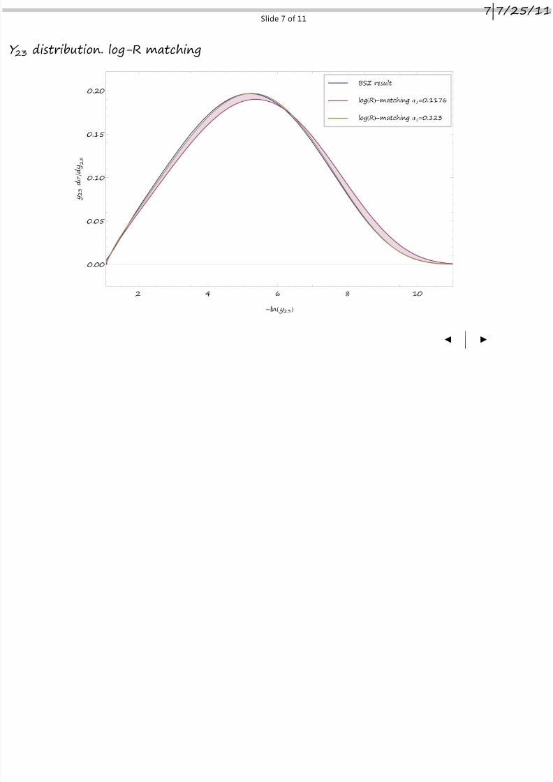
Y 23 distribution. log-R matching

|

7|7/25/11

| / /



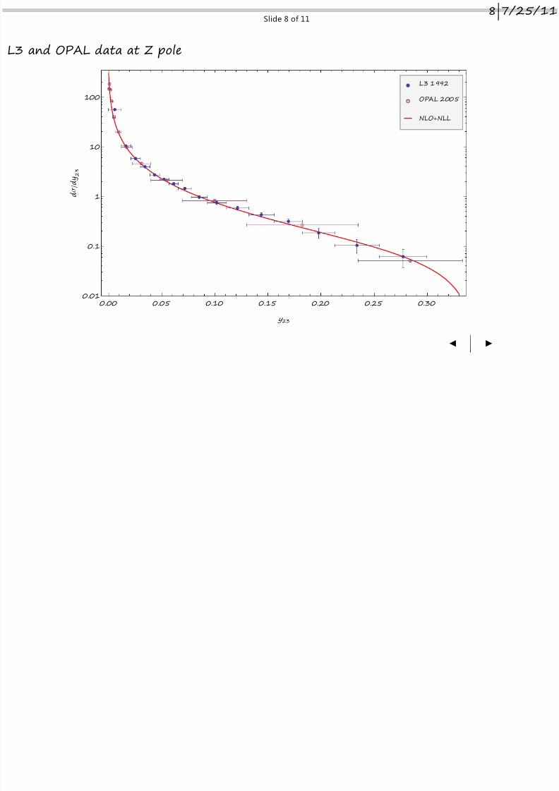
Slide 8 of 11

L3 and OPAL data at Z pole

0.00 0.05 0.10 0.15 0.20 0.25 0.300.01

0.1

1

10

100

y 23

d s ê d y 2 3

L3 1992

OPAL 2005

NLO+NLL

|

8|7/25/11

| /2 /11



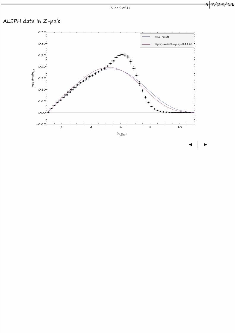
Slide 9 of 11

ALEPH data in Z-pole

2 4 6 8 10-0.05

0.00

0.05

0.10

0.15

0.20

0.25

0.30

0.35

-lnH y 23L

y 2 3

d s ê d y 2 3

BSZ result

logHRL-matching as =0.1176

|

9|7/25/11

10|7/25/11



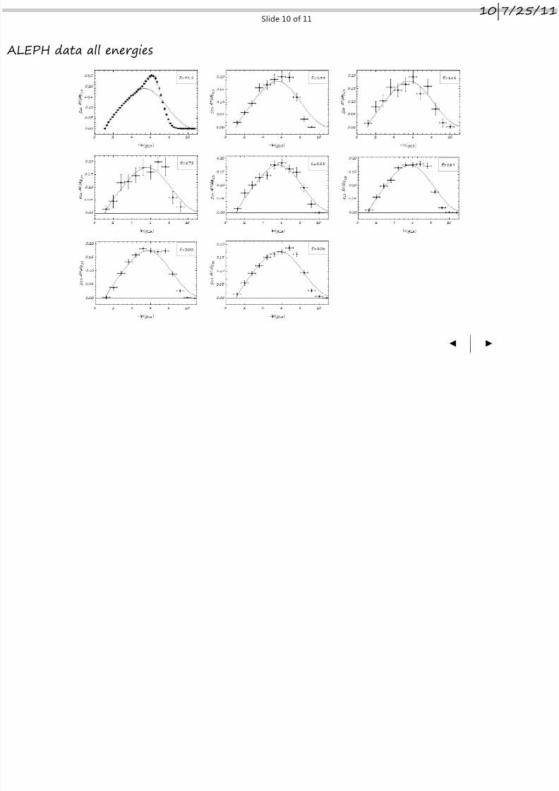
Slide 10 of 11

ALEPH data all energies

|

10|7/25/11

11|7/25/11



Slide 11 of 11

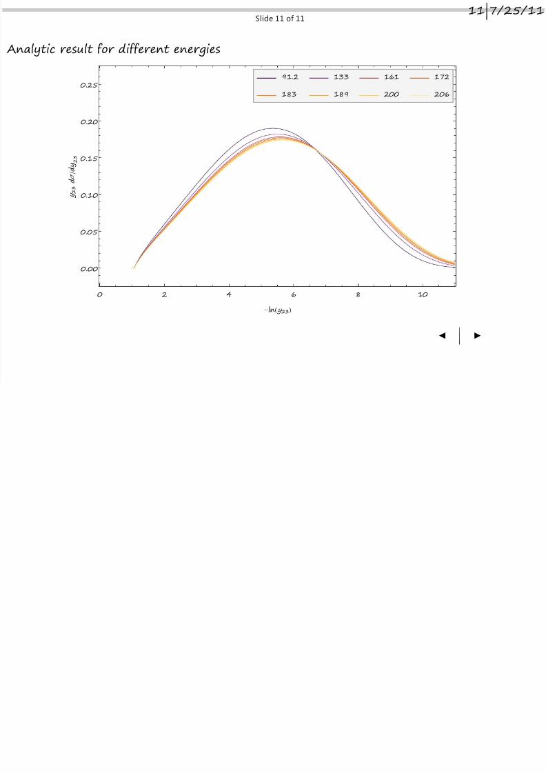
Analytic result for different energies

0 2 4 6 8 10

0.00

0.05

0.10

0.15

0.20

0.25

-lnH y 23L

y 2 3

d s ê d y 2 3

91.2 133 161 172

183 189 200 206

|

11|7/25/11

lecture 18, y23 distribution

Documents