lecture 19: chapter 8, section 1 sampling distributions...
TRANSCRIPT

©2011 Brooks/Cole, CengageLearning
Elementary Statistics: Looking at the Big Picture 1
Lecture 19: Chapter 8, Section 1Sampling Distributions:Proportions
Typical Inference ProblemDefinition of Sampling Distribution3 Approaches to Understanding Sampling Dist.Applying 68-95-99.7 Rule

©2011 Brooks/Cole,Cengage Learning
Elementary Statistics: Looking at the Big Picture L19.2
Looking Back: Review
4 Stages of Statistics Data Production (discussed in Lectures 1-4) Displaying and Summarizing (Lectures 5-12) Probability
Finding Probabilities (discussed in Lectures 13-14) Random Variables (discussed in Lectures 15-18) Sampling Distributions
Proportions Means
Statistical Inference

©2011 Brooks/Cole,Cengage Learning
Elementary Statistics: Looking at the Big Picture L19.3
Typical Inference ProblemIf sample of 100 students has 0.13 left-handed,can you believe population proportion is 0.10?Solution Method: Assume (temporarily) thatpopulation proportion is 0.10, find probabilityof sample proportion as high as 0.13. If it’s tooimprobable, we won’t believe populationproportion is 0.10.

©2011 Brooks/Cole,Cengage Learning
Elementary Statistics: Looking at the Big Picture L19.4
Key to Solving Inference ProblemsFor a given population proportion p and
sample size n, need to find probability ofsample proportion in a certain range:
Need to know sampling distribution of .Note: can denote a single statistic or a
random variable.

©2011 Brooks/Cole,Cengage Learning
Elementary Statistics: Looking at the Big Picture L19.5
DefinitionSampling distribution of sample statistic
tells probability distribution of valuestaken by the statistic in repeated randomsamples of a given size.
Looking Back: We summarize a probabilitydistribution by reporting its center,spread, shape.

©2011 Brooks/Cole,Cengage Learning
Elementary Statistics: Looking at the Big Picture L19.6
Behavior of Sample Proportion (Review)For random sample of size n from population
with p in category of interest, sampleproportion has
mean p standard deviation shape approximately normal for large
enough nLooking Back: Can find normal probabilitiesusing 68-95-99.7 Rule, etc.

©2011 Brooks/Cole,Cengage Learning
Elementary Statistics: Looking at the Big Picture L19.7
Rules of Thumb (Review) Population at least 10 times sample size n
(formula for standard deviation ofapproximately correct even if sampledwithout replacement)
np and n(1-p) both at least 10(guarantees approximately normal)

©2011 Brooks/Cole,Cengage Learning
Elementary Statistics: Looking at the Big Picture L19.8
Understanding Dist. of Sample Proportion3 Approaches:1. Intuition2. Hands-on Experimentation3. Theoretical Results
Looking Ahead: We’ll find that our intuition isconsistent with experimental results, and bothare confirmed by mathematical theory.

©2011 Brooks/Cole,Cengage Learning
Elementary Statistics: Looking at the Big Picture L19.10
Example: Shape of Underlying Distribution (n=1)
Background: Population proportion of blueM&M’s is p=1/6=0.17.
Question: How does the probability histogram forsample proportions appear for samples of size 1?
Response: ______________
for n=1
5/6
1/6
0 1
Looking Ahead: The shapeof the underlying distributionwill play a role in the shapeof for various sample sizes.

©2011 Brooks/Cole,Cengage Learning
Elementary Statistics: Looking at the Big Picture L19.12
Example: Sample Proportion as Random Variable
Background: Population proportion of blue M&Ms is 0.17. Questions:
Is the underlying variable categorical or quantitative? Consider the behavior of sample proportion for repeated random
samples of a given size. What type of variable is sample proportion? What 3 aspects of the distribution of sample proportion should we
report to summarize its behavior?
Responses: Underlying variable ______________________________________ _____________________________ Summarize with ___________, ___________, ___________

©2011 Brooks/Cole,Cengage Learning
Elementary Statistics: Looking at the Big Picture L19.14
Example: Center, Spread of Sample Proportion
Background: Population proportion of blue M&M’s isp=1/6=0.17.
Question: What can we say about center and spread of forrepeated random samples of size n = 25 (a teaspoon)?
Response: Center:
Spread of ’s: For n=6, could easily get anywhere from ___to ___. For n=25, spread of will be ____than it is for n = 6.
Some ’s more than ___, others less; shouldbalance out so mean of ’s is p = _______.
s.d. depends on ____.

©2011 Brooks/Cole,Cengage Learning
Elementary Statistics: Looking at the Big Picture L19.16
Example: Intuit Shape of Sample Proportion
Background: Population proportion of blue M&M’s isp=1/6=0.17.
Question: What can we say about the shape of forrepeated random samples of size n = 25 (a teaspoon)?
Response: close to____ most common, far from _____ in eitherdirection increasingly less likely_______________________________________________

©2011 Brooks/Cole,Cengage Learning
Elementary Statistics: Looking at the Big Picture L19.18
Example: Sample Proportion for Larger n
Background: Population proportion of blue M&M’s isp=1/6=0.17.
Question: What can we say about center, spread, shape offor repeated random samples of size n = 75 (a Tablespoon)?
Response: Center: Spread of ’s: compared to n=25, spread for n=75 is ____ Shape: ’s clumped near 0.17, taper at tails _________
mean of ’s should be p = _____ (for any n).
Looking Ahead: Sample size does not affect center but plays an important role inspread and shape of the distribution of sample proportion (also of sample mean).
©2011 Brooks/Cole,Cengage Learning
Elementary Statistics: Looking at the Big Picture L19.19
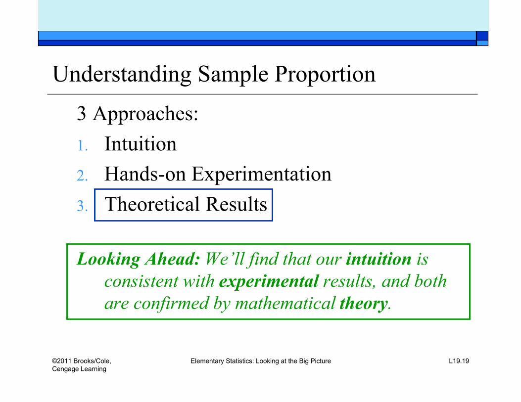
Understanding Sample Proportion3 Approaches:1. Intuition2. Hands-on Experimentation3. Theoretical Results
Looking Ahead: We’ll find that our intuition isconsistent with experimental results, and bothare confirmed by mathematical theory.

©2011 Brooks/Cole,Cengage Learning
Elementary Statistics: Looking at the Big Picture L19.20
Central Limit TheoremApproximate normality of sample statistic for
repeated random samples of a large enoughsize is cornerstone of inference theory.
Makes intuitive sense. Can be verified with experimentation. Proof requires higher-level mathematics;
result called Central Limit Theorem.

©2011 Brooks/Cole,Cengage Learning
Elementary Statistics: Looking at the Big Picture L19.21
Center of Sample Proportion (Implications)
For random sample of size n from populationwith p in category of interest, sampleproportion has
mean p is unbiased estimator of p
(sample must be random)

©2011 Brooks/Cole,Cengage Learning
Elementary Statistics: Looking at the Big Picture L19.22
Spread of Sample Proportion (Implications)
For random sample of size n from populationwith p in category of interest, sampleproportion has
mean p standard deviation
has less spread for larger samples(population size must be at least 10n)
n in denominator

©2011 Brooks/Cole,Cengage Learning
Elementary Statistics: Looking at the Big Picture L19.23
Shape of Sample Proportion (Implications)
For random sample of size n from populationwith p in category of interest, sampleproportion has
mean p standard deviation shape approx. normal for large enough n
can find probability that sampleproportion takes value in given interval

©2011 Brooks/Cole,Cengage Learning
Elementary Statistics: Looking at the Big Picture L19.25
Example: Behavior of Sample Proportion
Background: Population proportion of blueM&M’s is p=0.17.
Question: For repeated random samples of n=25,how does behave?
Response: For n=25, has Center: Spread: standard deviation _________________ Shape: not really normal because
___________________________
mean ________

©2011 Brooks/Cole,Cengage Learning
Elementary Statistics: Looking at the Big Picture L19.27
Example: Sample Proportion for Larger n
Background: Population proportion of blueM&M’s is p=0.17.
Question: For repeated random samples of n=75,how does behave?
Response: For n=75, has Center: Spread: standard deviation _________________ Shape: approximately normal because__________________________________________
mean ________

©2011 Brooks/Cole,Cengage Learning
Elementary Statistics: Looking at the Big Picture L19.28
68-95-99.7 Rule for Normal R.V. (Review)Sample at random from normal population; for sampled value X
(a R.V.), probability is 68% that X is within 1 standard deviation of mean 95% that X is within 2 standard deviations of mean 99.7% that X is within 3 standard deviations of mean

©2011 Brooks/Cole,Cengage Learning
Elementary Statistics: Looking at the Big Picture L19.29
68-95-99.7 Rule for Sample ProportionFor sample proportions taken at random from alarge population with underlying p, probability is 68% that is within 1 of p
95% that is within 2 of p
99.7% that is within 3 of p

©2011 Brooks/Cole,Cengage Learning
Elementary Statistics: Looking at the Big Picture L19.31
Example: Sample Proportion for n=75, p=0.17
Background: Population proportion of blue M&Msis p=0.17. For random samples of n=75, approx.normal with mean 0.17, s.d.
Question:What does 68-95-99.7 Rule tell us about behavior of ? Response: The probability is approximately
0.68 that is within _______ of ____: in (0.13, 0.21) 0.95 that is within _______ of ____: in (0.08, 0.26) 0.997 that is within _______ of ____: in (0.04, 0.30)
Looking Back: We don’t use the Rule for n=25 because ____________________

©2011 Brooks/Cole,Cengage Learning
Elementary Statistics: Looking at the Big Picture L19.32
90-95-98-99 Rule (Review)For standard normal Z, the probability is 0.90 that Z takes a value in interval (-1.645, +1.645) 0.95 that Z takes a value in interval (-1.960, +1.960) 0.98 that Z takes a value in interval (-2.326, +2.326) 0.99 that Z takes a value in interval (-2.576, +2.576)

©2011 Brooks/Cole,Cengage Learning
Elementary Statistics: Looking at the Big Picture L19.34
Example: Sample Proportion for n=75, p=0.17
Background: Population proportion of blue M&Msis p=0.17. For random samples of n=75, approx.normal with mean 0.17, s.d.
Question:What does 90-95-98-99 Rule tell about behavior of ? Response: The probability is approximately
0.90 that is within _____(0.043) of 0.17: in (0.10,0.24) 0.95 that is within _____(0.043) of 0.17: in (0.09,0.25) 0.98 that is within _____(0.043) of 0.17: in (0.07,0.27) 0.99 that is within _____(0.043) of 0.17: in (0.06,0.28)

©2011 Brooks/Cole,Cengage Learning
Elementary Statistics: Looking at the Big Picture L19.35
Typical Inference Problem (Review)If sample of 100 students has 0.13 left-handed,can you believe population proportion is 0.10?Solution Method: Assume (temporarily) thatpopulation proportion is 0.10, find probabilityof sample proportion as high as 0.13. If it’s tooimprobable, we won’t believe populationproportion is 0.10.

©2011 Brooks/Cole,Cengage Learning
Elementary Statistics: Looking at the Big Picture L19.37
Example: Testing Assumption About p Background: We asked, “If sample of 100 students has 0.13
left-handed, can you believe population proportion is 0.10?” Questions:
What are the mean, standard deviation, and shape of ? Is 0.13 improbably high under the circumstances? Can we believe p = 0.10?
Response: For p=0.10 and n=100, has mean ____, s.d. ________________ ;
shape approx. normal since _________________________________. According to Rule, the probability is _______________ that would
take a value of 0.13 (1 s.d. above mean) or more. Since this isn’t so improbable, ______________________________.

©2011 Brooks/Cole,Cengage Learning
Elementary Statistics: Looking at the Big Picture L19.38
Lecture Summary(Distribution of Sample Proportion) Typical inference problem Sampling distribution; definition 3 approaches to understanding sampling dist.
Intuition Hands-on experiment Theory
Center, spread, shape of sampling distribution Central Limit Theorem
Role of sample size Applying 68-95-99.7 Rule