lecture 2-2
DESCRIPTION
as a matter of the company’s policy?TRANSCRIPT

© 2014 Pearson Education, Inc. S6 - 1
Statistical Process Control

© 2014 Pearson Education, Inc. S6 - 2
Outline
► Statistical Process Control► Process Capability► Acceptance Sampling
© 2014 Pearson Education, Inc. S6 - 3
Learning ObjectivesWhen you complete this supplement you should be able to :1. Explain the purpose of a control chart2. Explain the role of the central limit theorem
in SPC3. Build -charts and R-charts4. List the five steps involved in building
control charts

© 2014 Pearson Education, Inc. S6 - 4
Learning ObjectivesWhen you complete this supplement you should be able to :5. Build p-charts and c-charts
6. Explain process capability and compute Cp and Cpk
7. Explain acceptance sampling

© 2014 Pearson Education, Inc. S6 - 5
Statistical Process Control
The objective of a process control system is to provide a statistical
signal when assignable causes of variation are present
© 2014 Pearson Education, Inc. S6 - 6
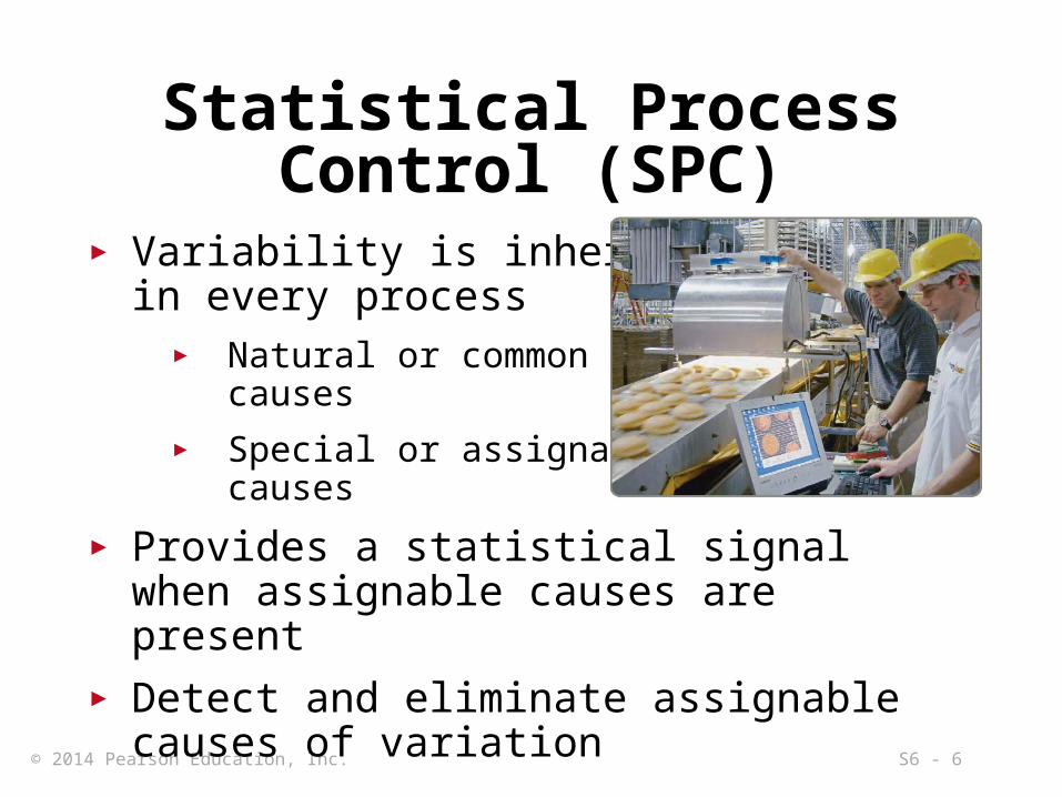
► Variability is inherent in every process
► Natural or common causes
► Special or assignable causes
► Provides a statistical signal when assignable causes are present
► Detect and eliminate assignable causes of variation
Statistical Process Control (SPC)

© 2014 Pearson Education, Inc. S6 - 7
Common Causes▶Common causes of variation are the purely
random, unidentifiable sources of variation that are unavoidable with the current process. For example, the time required to process specimens at an intensive care unit lab in a hospital will vary. If time is measured to complete an analysis for a large no. of patients and plotted the results, the data would tend to form a pattern that can be
described as a distribution.

© 2014 Pearson Education, Inc. S6 - 8
Natural Variations► Also called common causes► Affect virtually all production processes► Expected amount of variation► Output measures follow a probability
distribution► For any distribution there is a measure of
central tendency and dispersion► If the distribution of outputs falls within
acceptable limits, the process is said to be “in control”

© 2014 Pearson Education, Inc. S6 - 9
Common Causes▶A distribution may be characterized by its mean, spread, and shape.
▶ The spread is a measure of the dispersion of observations about the mean. The standard deviation is the square root of the variance of a distribution.
x xi
i1
n
n
xi x 2
n 1
Mean Standard Deviation/ Spread

© 2014 Pearson Education, Inc. S6 - 10
Assignable Variations► Also called special causes of variation
► Generally this is some change in the process► Variations that can be traced to a specific
reason► The objective is to discover when assignable
causes are present► Eliminate the bad causes► Incorporate the good causes

© 2014 Pearson Education, Inc. S6 - 11
Assignable CausesAssignable Causes
(a) Location(a) Location TimeTime Figure 6.0Figure 6.0
AverageAverage
The green curve is the process distribution when only common The green curve is the process distribution when only common causes of variation are present. The red lines depict a change in causes of variation are present. The red lines depict a change in the distribution because of assignable causes. In Fig. 6.0(a) the the distribution because of assignable causes. In Fig. 6.0(a) the red line indicates that the process took more time than planned red line indicates that the process took more time than planned in many of the cases, thereby increasing the average time of in many of the cases, thereby increasing the average time of each analysis. each analysis.

© 2014 Pearson Education, Inc. S6 - 12
Assignable CausesAssignable Causes
(b) Spread(b) SpreadTimeTime
AverageAverage
Figure 6.0Figure 6.0
An increase in the variability of the time for each case An increase in the variability of the time for each case affected the spread of the distribution.affected the spread of the distribution.

© 2014 Pearson Education, Inc. S6 - 13
Assignable CausesAssignable Causes
(c) Shape(c) Shape TimeTime
AverageAverage
Figure 6.0Figure 6.0
The red line indicates that the process produced a The red line indicates that the process produced a preponderance of the tests in less than average time. preponderance of the tests in less than average time.
A process is said to be in statistical control when the A process is said to be in statistical control when the location, spread, or shape of its distribution does not location, spread, or shape of its distribution does not change over time.change over time.
© 2014 Pearson Education, Inc. S6 - 14
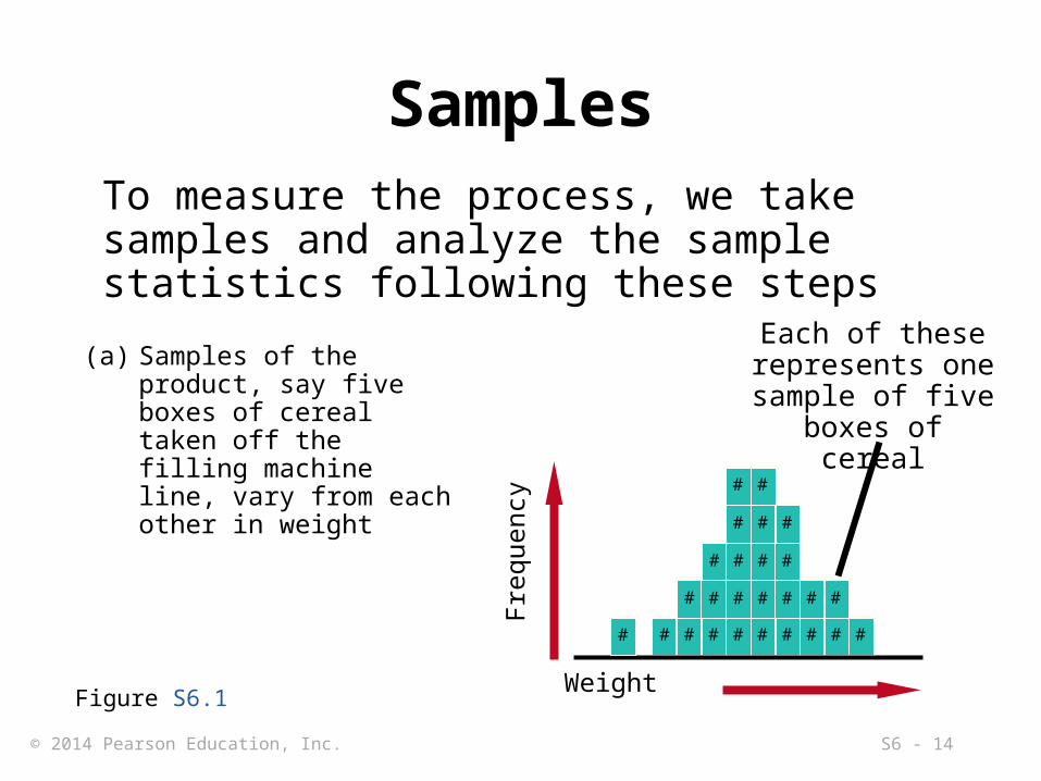
SamplesTo measure the process, we take samples and analyze the sample statistics following these steps
(a) Samples of the product, say five boxes of cereal taken off the filling machine line, vary from each other in weight
Freq
uenc
y
Weight
#
## #
##
##
#
# # ## # ##
# # ## # ## # ##
Each of these represents one sample of five
boxes of cereal
Figure S6.1

© 2014 Pearson Education, Inc. S6 - 15
SamplesTo measure the process, we take samples and analyze the sample statistics following these steps
(b) After enough samples are taken from a stable process, they form a pattern called a distribution
The solid line represents the
distribution
Freq
uenc
y
WeightFigure S6.1

© 2014 Pearson Education, Inc. S6 - 16
Samples
(c) There are many types of distributions, including the normal (bell-shaped) distribution, but distributions do differ in terms of central tendency (mean), standard deviation or variance, and shape
Weight
Central tendency
Weight
Variation
Weight
Shape
Freq
uenc
y
Figure S6.1
To measure the process, we take samples and analyze the sample statistics following these steps

© 2014 Pearson Education, Inc. S6 - 17
SamplesTo measure the process, we take samples and analyze the sample statistics following these steps
(d) If only natural causes of variation are present, the output of a process forms a distribution that is stable over time and is predictable
WeightTimeFr
eque
ncy Prediction
Figure S6.1

© 2014 Pearson Education, Inc. S6 - 18
SamplesTo measure the process, we take samples and analyze the sample statistics following these steps
(e) If assignable causes are present, the process output is not stable over time and is not predicable
WeightTimeFr
eque
ncy Prediction
????
???
???
??????
???
Figure S6.1

© 2014 Pearson Education, Inc. S6 - 19
Control ChartsConstructed from historical data, the purpose of control charts is to help distinguish between natural variations and variations due to assignable causes

© 2014 Pearson Education, Inc. S6 - 20
Process Control
Figure S6.2
Frequency
(weight, length, speed, etc.)Size
Lower control limit Upper control limit
(a) In statistical control and capable of producing within control limits
(b) In statistical control but not capable of producing within control limits
(c) Out of control

© 2014 Pearson Education, Inc. S6 - 21
Control Charts for Variables
► Characteristics that can take any real value► May be in whole or in fractional numbers► Continuous random variables
x-chart tracks changes in the central tendency
R-chart indicates a gain or loss of dispersion These two charts
must be used
together

© 2014 Pearson Education, Inc. S6 - 22
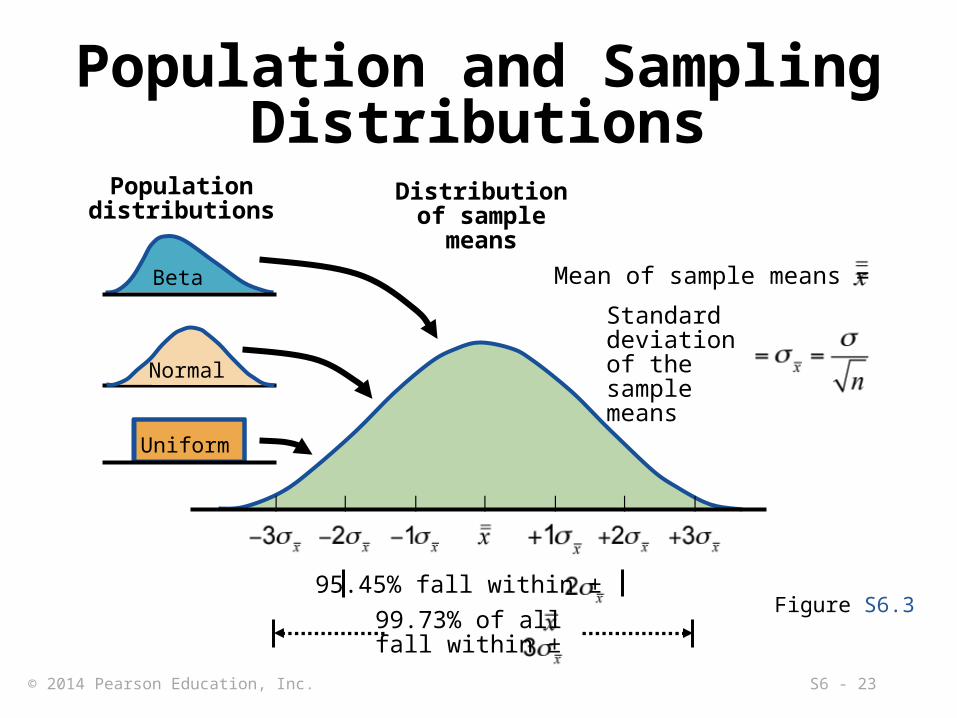
Central Limit TheoremRegardless of the distribution of the population, the distribution of sample means drawn from the population will tend to follow a normal curve
2) The standard deviation of the sampling distribution ( ) will equal the population standard deviation () divided by the square root of the sample size, n
1) The mean of the sampling distribution will be the same as the population mean
© 2014 Pearson Education, Inc. S6 - 23
Population and Sampling Distributions
Population distributions
Beta
Normal
Uniform
Distribution of sample means
Figure S6.399.73% of allfall within ±
95.45% fall within ±
| | | | | | |
Standard deviation of the sample means
Mean of sample means =
© 2014 Pearson Education, Inc. S6 - 24
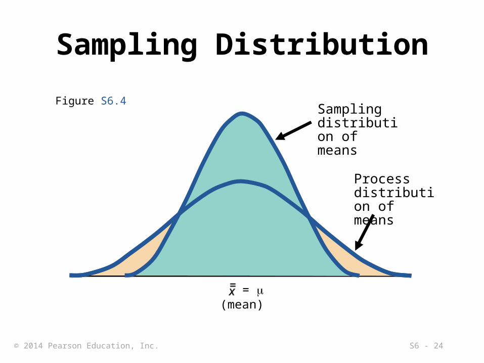
Sampling Distribution
= (mean)
Sampling distribution of means
Process distribution of means
Figure S6.4

© 2014 Pearson Education, Inc. S6 - 25
Setting Chart LimitsFor x-Charts when we know
Where =mean of the sample means or a target value set for the processz =number of normal standard deviationsx =standard deviation of the sample means =population (process) standard deviationn =sample size

© 2014 Pearson Education, Inc. S6 - 26
Setting Control Limits▶Randomly select and weigh nine (n = 9) boxes
each hour
WEIGHT OF SAMPLE WEIGHT OF SAMPLE WEIGHT OF SAMPLE
HOUR(AVG. OF 9
BOXES) HOUR(AVG. OF 9
BOXES) HOUR(AVG. OF 9
BOXES)1 16.1 5 16.5 9 16.3
2 16.8 6 16.4 10 14.8
3 15.5 7 15.2 11 14.2
4 16.5 8 16.4 12 17.3
Average weight in the first sample

© 2014 Pearson Education, Inc. S6 - 27
Setting Control Limits
Average mean of 12 samples

© 2014 Pearson Education, Inc. S6 - 28
Setting Control Limits
Average mean of 12 samples

© 2014 Pearson Education, Inc. S6 - 29
17 = UCL
15 = LCL
16 = Mean
Sample number
| | | | | | | | | | | |1 2 3 4 5 6 7 8 9 10 11 12
Setting Control LimitsControl Chart for samples of 9 boxes
Variation due to assignable
causes
Variation due to assignable
causes
Variation due to natural causes
Out of control
Out of control

© 2014 Pearson Education, Inc. S6 - 30
Setting Chart Limits
For x-Charts when we don’t know
where average range of the samples
A2 =control chart factor found in Table S6.1
=mean of the sample means

© 2014 Pearson Education, Inc. S6 - 31
Control Chart FactorsTABLE S6.1 Factors for Computing Control Chart Limits (3 sigma)
SAMPLE SIZE, n
MEAN FACTOR, A2
UPPER RANGE, D4
LOWER RANGE, D3
2 1.880 3.268 0
3 1.023 2.574 0
4 .729 2.282 0
5 .577 2.115 0
6 .483 2.004 0
7 .419 1.924 0.076
8 .373 1.864 0.136
9 .337 1.816 0.184
10 .308 1.777 0.223
12 .266 1.716 0.284

© 2014 Pearson Education, Inc. S6 - 32
Setting Control LimitsProcess average = 12 ouncesAverage range = .25 ounceSample size = 5
UCL = 12.144
Mean = 12
LCL = 11.856
From Table S6.1
Super Cola ExampleLabeled as “net weight 12 ounces”
© 2014 Pearson Education, Inc. S6 - 33
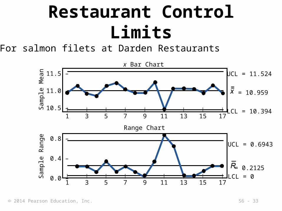
Restaurant Control LimitsFor salmon filets at Darden Restaurants
Sam
ple
Mea
n
x Bar ChartUCL = 11.524
= 10.959
LCL = 10.394| | | | | | | | |1 3 5 7 9 11 13 15 17
11.5 –
11.0 –
10.5 –
Sam
ple
Ran
ge
Range Chart
UCL = 0.6943
= 0.2125LCL = 0| | | | | | | | |
1 3 5 7 9 11 13 15 17
0.8 –
0.4 –
0.0 –

© 2014 Pearson Education, Inc. S6 - 34
R – Chart► Type of variables control chart► Shows sample ranges over time
► Difference between smallest and largest values in sample
► Monitors process variability► Independent from process mean

© 2014 Pearson Education, Inc. S6 - 35
Setting Chart LimitsFor R-Charts
where

© 2014 Pearson Education, Inc. S6 - 36
Setting Control LimitsAverage range = 5.3 poundsSample size = 5From Table S6.1 D4 = 2.115, D3 = 0
UCL = 11.2
Mean = 5.3
LCL = 0

© 2014 Pearson Education, Inc. S6 - 37
Mean and Range Charts(a)These sampling distributions result in the charts below
(Sampling mean is shifting upward, but range is consistent)
R-chart(R-chart does not detect change in mean)
UCL
LCLFigure S6.5
x-chart(x-chart detects shift in central tendency)
UCL
LCL

© 2014 Pearson Education, Inc. S6 - 38
Mean and Range Charts
R-chart(R-chart detects increase in dispersion)
UCL
LCL
(b)These sampling distributions result in the charts below
(Sampling mean is constant, but dispersion is increasing)
x-chart(x-chart indicates no change in central tendency)
UCL
LCL
Figure S6.5

© 2014 Pearson Education, Inc. S6 - 39
Steps In Creating Control Charts
1. Collect 20 to 25 samples, often of n = 4 or n = 5 observations each, from a stable process and compute the mean and range of each
2. Compute the overall means ( and ), set appropriate control limits, usually at the 99.73% level, and calculate the preliminary upper and lower control limits► If the process is not currently stable and in control, use
the desired mean, , instead of to calculate limits.

© 2014 Pearson Education, Inc. S6 - 40
Steps In Creating Control Charts
3. Graph the sample means and ranges on their respective control charts and determine whether they fall outside the acceptable limits
4. Investigate points or patterns that indicate the process is out of control – try to assign causes for the variation, address the causes, and then resume the process
5. Collect additional samples and, if necessary, revalidate the control limits using the new data

© 2014 Pearson Education, Inc. S6 - 41
Setting Other Control Limits
TABLE S6.2 Common z Values
DESIRED CONTROL LIMIT (%)
Z-VALUE (STANDARD DEVIATION REQUIRED
FOR DESIRED LEVEL OF CONFIDENCE
90.0 1.65
95.0 1.96
95.45 2.00
99.0 2.58
99.73 3.00

© 2014 Pearson Education, Inc. S6 - 42
Control ChartsControl Chartsfor Variablesfor Variables
West Allis IndustriesWest Allis Industries
Example
The management of West Allis Industries is concerned about the production of a special metal screw used by several of the company’s largest customers. The diameter of the screw is critical to the customers. Data from five samples appear in the accompanying table. The sample size is 4. Is the process in statistical control?

© 2014 Pearson Education, Inc. S6 - 43
Control ChartsControl Chartsfor Variablesfor Variables
ExampleExample
Sample SampleNumber 1 2 3 4 R x
1 0.5014 0.5022 0.5009 0.50272 0.5021 0.5041 0.5024 0.50203 0.5018 0.5026 0.5035 0.50234 0.5008 0.5034 0.5024 0.50155 0.5041 0.5056 0.5034 0.5039
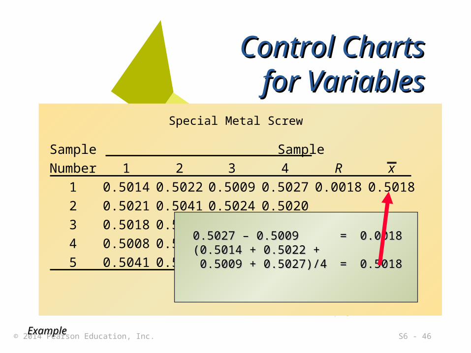
Special Metal Screw
_

© 2014 Pearson Education, Inc. S6 - 44
Control ChartsControl Chartsfor Variablesfor Variables
Example Example
Sample SampleNumber 1 2 3 4 R x
1 0.5014 0.5022 0.5009 0.5027 0.0018 0.50182 0.5021 0.5041 0.5024 0.50203 0.5018 0.5026 0.5035 0.50234 0.5008 0.5034 0.5024 0.50155 0.5041 0.5056 0.5034 0.5039
Special Metal Screw
_
0.5027 – 0.50090.5027 – 0.5009 == 0.00180.0018

© 2014 Pearson Education, Inc. S6 - 45
Control ChartsControl Chartsfor Variablesfor Variables
Example Example
Sample SampleNumber 1 2 3 4 R x
1 0.5014 0.5022 0.5009 0.5027 0.0018 0.50182 0.5021 0.5041 0.5024 0.50203 0.5018 0.5026 0.5035 0.50234 0.5008 0.5034 0.5024 0.50155 0.5041 0.5056 0.5034 0.5039
Special Metal Screw
_
0.5027 – 0.50090.5027 – 0.5009 == 0.00180.0018
© 2014 Pearson Education, Inc. S6 - 46
Control ChartsControl Chartsfor Variablesfor Variables
Example Example
Sample SampleNumber 1 2 3 4 R x
1 0.5014 0.5022 0.5009 0.5027 0.0018 0.50182 0.5021 0.5041 0.5024 0.50203 0.5018 0.5026 0.5035 0.50234 0.5008 0.5034 0.5024 0.50155 0.5041 0.5056 0.5034 0.5039
Special Metal Screw
_
(0.5014 + 0.5022 +(0.5014 + 0.5022 + 0.5009 + 0.5027)/40.5009 + 0.5027)/4 == 0.50180.5018
0.5027 – 0.50090.5027 – 0.5009 == 0.00180.0018

© 2014 Pearson Education, Inc. S6 - 47
Control ChartsControl Chartsfor Variablesfor Variables
Sample SampleNumber 1 2 3 4 R x
1 0.5014 0.5022 0.5009 0.5027 0.0018 0.50182 0.5021 0.5041 0.5024 0.5020 0.0021 0.50273 0.5018 0.5026 0.5035 0.5023 0.0017 0.50264 0.5008 0.5034 0.5024 0.5015 0.0026 0.50205 0.5041 0.5056 0.5034 0.5047 0.0022 0.5045
R = 0.0021x = 0.5027
Special Metal Screw
Example Example
=
_

© 2014 Pearson Education, Inc. S6 - 48Example 5.1Example 5.1
Control ChartsControl Chartsfor Variablesfor Variables
Control Charts – Special Metal Screw
R-Charts R = 0.0021
UCLR = D4RLCLR = D3R

© 2014 Pearson Education, Inc. S6 - 49Example 5.1Example 5.1
Control ChartsControl Chartsfor Variablesfor VariablesTable 5.1 Control Chart FactorsTable 5.1 Control Chart Factors
Factor for UCLFactor for UCL Factor forFactor for FactorFactorSize ofSize of and LCL forand LCL for LCL forLCL for UCL forUCL forSampleSample xx-Charts-Charts RR-Charts-Charts RR-Charts-Charts
((nn)) ((AA22)) ((DD33)) ((DD44))
22 1.8801.880 0 0 3.2673.26733 1.0231.023 0 0 2.5752.57544 0.7290.729 0 0 2.2822.28255 0.5770.577 0 0 2.1152.11566 0.4830.483 0 0 2.0042.00477 0.4190.419 0.0760.076 1.9241.92488 0.3730.373 0.1360.136 1.8641.86499 0.3370.337 0.1840.184 1.8161.8161010 0.3080.308 0.2230.223 1.7771.777

© 2014 Pearson Education, Inc. S6 - 50Example 5.1Example 5.1
Control ChartsControl Chartsfor Variablesfor Variables
Control Charts – Special Metal Screw
R-Charts R = 0.0021
UCLR = D4RLCLR = D3R
© 2014 Pearson Education, Inc. S6 - 51Example 5.1Example 5.1
Control ChartsControl Chartsfor Variablesfor Variables
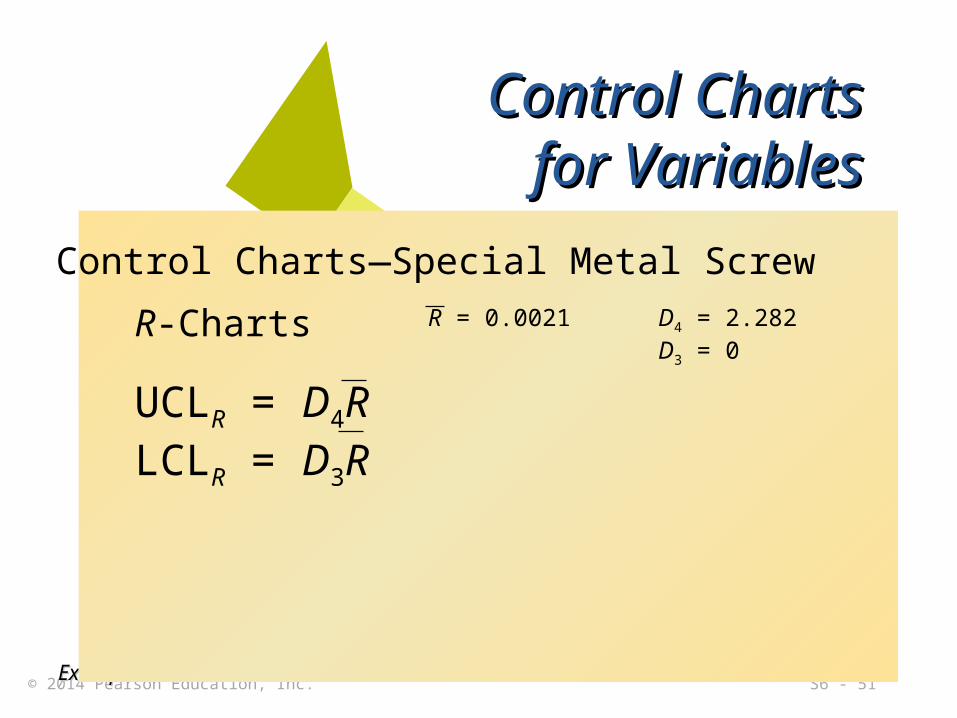
Control Charts—Special Metal Screw
R-Charts R = 0.0021 D4 = 2.282D3 = 0
UCLR = D4RLCLR = D3R

© 2014 Pearson Education, Inc. S6 - 52Example 5.1Example 5.1
Control ChartsControl Chartsfor Variablesfor Variables
Control Charts—Special Metal Screw
R-Charts R = 0.0021 D4 = 2.282D3 = 0
UCLR = 2.282 (0.0021) = 0.00479 in.
UCLR = D4RLCLR = D3R

© 2014 Pearson Education, Inc. S6 - 53Example 5.1Example 5.1
Control ChartsControl Chartsfor Variablesfor Variables
Control Charts—Special Metal Screw
R-Charts R = 0.0021 D4 = 2.282D3 = 0
UCLR = 2.282 (0.0021) = 0.00479 in.LCLR = 0 (0.0021) = 0 in.
UCLR = D4RLCLR = D3R

© 2014 Pearson Education, Inc. S6 - 54Example 5.1Example 5.1
Control ChartsControl Chartsfor Variablesfor Variables
Control Charts—Special Metal Screw
R-Charts R = 0.0021 D4 = 2.282D3 = 0
UCLR = 2.282 (0.0021) = 0.00479 in.LCLR = 0 (0.0021) = 0 in.
UCLR = D4RLCLR = D3R

© 2014 Pearson Education, Inc. S6 - 55
Range Chart - Special Metal Screw
ExampleExample

© 2014 Pearson Education, Inc. S6 - 56Example 5.1Example 5.1
Control ChartsControl Chartsfor Variablesfor Variables
Control Charts—Special Metal Screw
X-Charts
UCLx = x + A2RLCLx = x - A2R
==
R = 0.0021x = 0.5027=

© 2014 Pearson Education, Inc. S6 - 57Example 5.1Example 5.1
Control ChartsControl Chartsfor Variablesfor Variables
Control Charts—Special Metal Screw
X-Charts
UCLx = x + A2RLCLx = x - A2R
==
R = 0.0021x = 0.5027=
Table 5.1 Control Chart FactorsTable 5.1 Control Chart Factors
Factor for UCLFactor for UCL Factor forFactor for FactorFactorSize ofSize of and LCL forand LCL for LCL forLCL for UCL forUCL forSampleSample xx-Charts-Charts RR-Charts-Charts RR-Charts-Charts
((nn)) ((AA22)) ((DD33)) ((DD44))
22 1.8801.880 0 0 3.2673.26733 1.0231.023 0 0 2.5752.57544 0.7290.729 0 0 2.2822.28255 0.5770.577 0 0 2.1152.11566 0.4830.483 0 0 2.0042.00477 0.4190.419 0.0760.076 1.9241.92488 0.3730.373 0.1360.136 1.8641.86499 0.3370.337 0.1840.184 1.8161.8161010 0.3080.308 0.2230.223 1.7771.777

© 2014 Pearson Education, Inc. S6 - 58Example 5.1Example 5.1
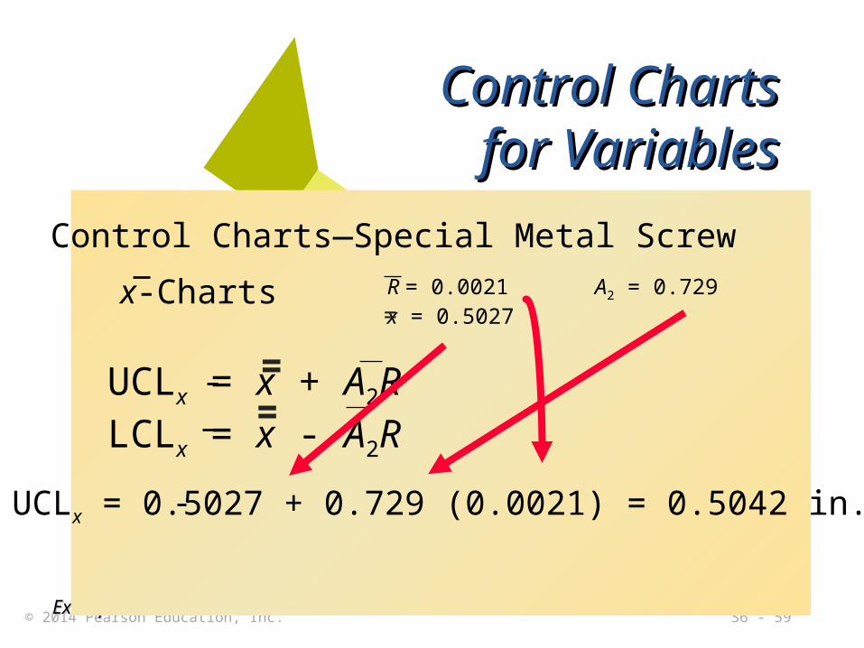
Control ChartsControl Chartsfor Variablesfor Variables
Control Charts—Special Metal Screw
x-Charts
UCLx = x + A2RLCLx = x - A2R
==
R = 0.0021 A2 = 0.729x = 0.5027=
© 2014 Pearson Education, Inc. S6 - 59Example 5.1Example 5.1
Control ChartsControl Chartsfor Variablesfor Variables
Control Charts—Special Metal Screw
x-Charts
UCLx = 0.5027 + 0.729 (0.0021) = 0.5042 in.
UCLx = x + A2RLCLx = x - A2R
==
R = 0.0021 A2 = 0.729x = 0.5027=

© 2014 Pearson Education, Inc. S6 - 60Example 5.1Example 5.1
Control ChartsControl Chartsfor Variablesfor Variables
Control Charts—Special Metal Screw
x-Charts
UCLx = 0.5027 + 0.729 (0.0021) = 0.5042 in.LCLx = 0.5027 – 0.729 (0.0021) = 0.5012 in.
UCLx = x + A2RLCLx = x - A2R
==
R = 0.0021 A2 = 0.729x = 0.5027=

© 2014 Pearson Education, Inc. S6 - 61
x-Chart—Special Metal Screw
Example Example
© 2014 Pearson Education, Inc. S6 - 62
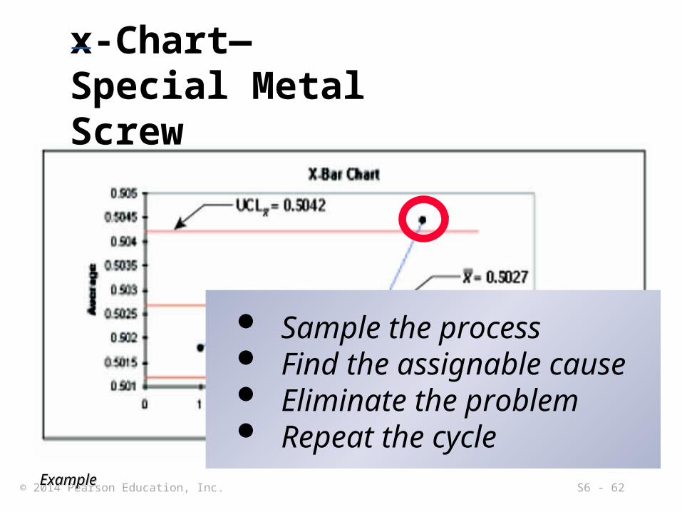
x-Chart—Special Metal Screw
Example Example
Sample the process Find the assignable cause Eliminate the problem Repeat the cycle

© 2014 Pearson Education, Inc. S6 - 63
Control Charts for Attributes► For variables that are categorical
► Defective/nondefective, good/bad, yes/no, acceptable/unacceptable
► Measurement is typically counting defectives
► Charts may measure1. Percent defective (p-chart)2. Number of defects (c-chart)

© 2014 Pearson Education, Inc. S6 - 64
Control Limits for p-ChartsPopulation will be a binomial distribution, but applying the Central Limit Theorem allows us
to assume a normal distribution for the sample statistics
where

© 2014 Pearson Education, Inc. S6 - 65
p-Chart for Data EntrySAMPLE NUMBER
NUMBER OF
ERRORSFRACTION DEFECTIVE
SAMPLE NUMBER
NUMBER OF
ERRORSFRACTION DEFECTIVE
1 6 .06 11 6 .06
2 5 .05 12 1 .01
3 0 .00 13 8 .08
4 1 .01 14 7 .07
5 4 .04 15 5 .05
6 2 .02 16 4 .04
7 5 .05 17 11 .11
8 3 .03 18 3 .03
9 3 .03 19 0 .00
10 2 .02 20 4 .04
80

© 2014 Pearson Education, Inc. S6 - 66
p-Chart for Data EntrySAMPLE NUMBER
NUMBER OF
ERRORSFRACTION DEFECTIVE
SAMPLE NUMBER
NUMBER OF
ERRORSFRACTION DEFECTIVE
1 6 .06 11 6 .06
2 5 .05 12 1 .01
3 0 .00 13 8 .08
4 1 .01 14 7 .07
5 4 .04 15 5 .05
6 2 .02 16 4 .04
7 5 .05 17 11 .11
8 3 .03 18 3 .03
9 3 .03 19 0 .00
10 2 .02 20 4 .04
80(because we cannot
have a negative
percent defective)

© 2014 Pearson Education, Inc. S6 - 67
.11 –
.10 –
.09 –
.08 –
.07 –
.06 –
.05 –
.04 –
.03 –
.02 –
.01 –
.00 –
Sample number
Frac
tion
defe
ctiv
e
| | | | | | | | | |
2 4 6 8 10 12 14 16 18 20
p-Chart for Data Entry
UCLp = 0.10
LCLp = 0.00
p = 0.04
© 2014 Pearson Education, Inc. S6 - 68
.11 –
.10 –
.09 –
.08 –
.07 –
.06 –
.05 –
.04 –
.03 –
.02 –
.01 –
.00 –
Sample number
Frac
tion
defe
ctiv
e
| | | | | | | | | |
2 4 6 8 10 12 14 16 18 20
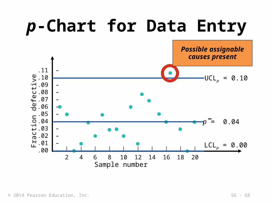
p-Chart for Data Entry
UCLp = 0.10
LCLp = 0.00
p = 0.04
Possible assignable causes present
© 2014 Pearson Education, Inc. S6 - 69
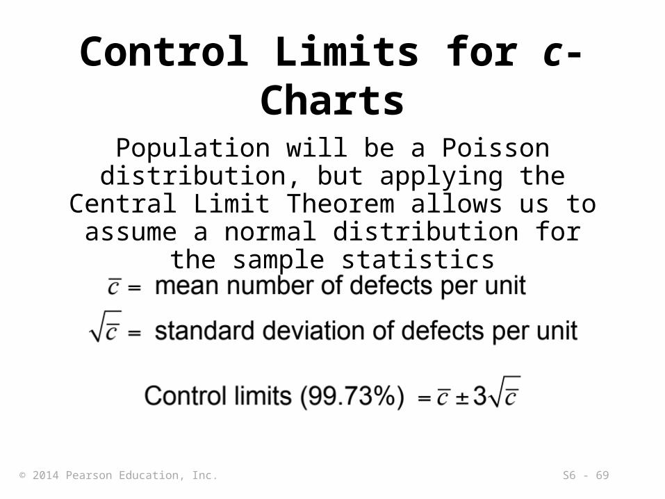
Control Limits for c-ChartsPopulation will be a Poisson distribution, but applying the Central Limit Theorem allows us
to assume a normal distribution for the sample statistics

© 2014 Pearson Education, Inc. S6 - 70
c-Chart for Cab Company
|1
|2
|3
|4
|5
|6
|7
|8
|9
Day
Num
ber d
efec
tive
14 –12 –10 –
8 –6 –4 –2 –0 –
UCLc = 13.35
LCLc = 0
c = 6
Cannot be a
negative number

© 2014 Pearson Education, Inc. S6 - 71
► Select points in the processes that need SPC
► Determine the appropriate charting technique
► Set clear policies and procedures
Managerial Issues andControl Charts
Three major management decisions:
© 2014 Pearson Education, Inc. S6 - 72
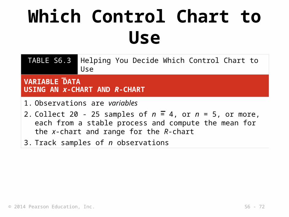
Which Control Chart to UseTABLE S6.3 Helping You Decide Which Control Chart to Use
VARIABLE DATAUSING AN x-CHART AND R-CHART
1. Observations are variables2. Collect 20 - 25 samples of n = 4, or n = 5, or more, each from a stable
process and compute the mean for the x-chart and range for the R-chart3. Track samples of n observations

© 2014 Pearson Education, Inc. S6 - 73
Which Control Chart to UseTABLE S6.3 Helping You Decide Which Control Chart to Use
ATTRIBUTE DATAUSING A P-CHART1. Observations are attributes that can be categorized as good or bad (or
pass–fail, or functional–broken), that is, in two states2. We deal with fraction, proportion, or percent defectives3. There are several samples, with many observations in each
ATTRIBUTE DATAUSING A C-CHART1. Observations are attributes whose defects per unit of output can be
counted2. We deal with the number counted, which is a small part of the possible
occurrences3. Defects may be: number of blemishes on a desk; crimes in a year;
broken seats in a stadium; typos in a chapter of this text; flaws in a bolt of cloth
© 2014 Pearson Education, Inc. S6 - 74
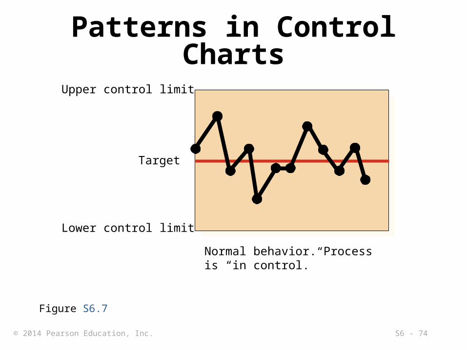
Patterns in Control Charts
Normal behavior. Process is “in control.”
Upper control limit
Target
Lower control limit
Figure S6.7

© 2014 Pearson Education, Inc. S6 - 75
Patterns in Control Charts
One plot out above (or below). Investigate for cause. Process is “out of control.”
Upper control limit
Target
Lower control limit
Figure S6.7

© 2014 Pearson Education, Inc. S6 - 76
Patterns in Control Charts
Trends in either direction, 5 plots. Investigate for cause of progressive change.
Upper control limit
Target
Lower control limit
Figure S6.7

© 2014 Pearson Education, Inc. S6 - 77
Patterns in Control Charts
Two plots very near lower (or upper) control. Investigate for cause.
Upper control limit
Target
Lower control limit
Figure S6.7

© 2014 Pearson Education, Inc. S6 - 78
Patterns in Control Charts
Run of 5 above (or below) central line. Investigate for cause.
Upper control limit
Target
Lower control limit
Figure S6.7
© 2014 Pearson Education, Inc. S6 - 79
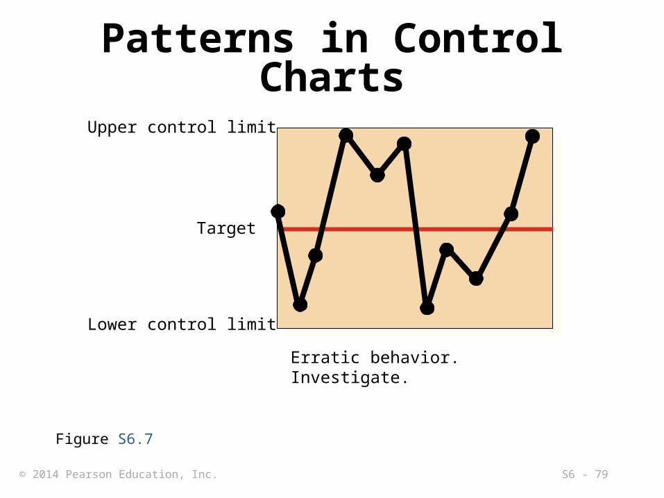
Patterns in Control Charts
Erratic behavior. Investigate.
Upper control limit
Target
Lower control limit
Figure S6.7

© 2014 Pearson Education, Inc. S6 - 80
Process Capability► The natural variation of a process should
be small enough to produce products that meet the standards required
► A process in statistical control does not necessarily meet the design specifications
► Process capability is a measure of the relationship between the natural variation of the process and the design specifications

© 2014 Pearson Education, Inc. S6 - 81
Process Capability RatioCp =
Upper Specification – Lower Specification6
► A capable process must have a Cp of at least 1.0
► Does not look at how well the process is centered in the specification range
► Often a target value of Cp = 1.33 is used to allow for off-center processes
► Six Sigma quality requires a Cp = 2.0

© 2014 Pearson Education, Inc. S6 - 82
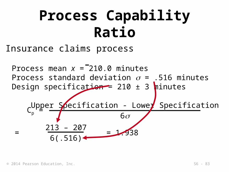
Process Capability Ratio
Cp = Upper Specification - Lower Specification6
Insurance claims process
Process mean x = 210.0 minutesProcess standard deviation = .516 minutesDesign specification = 210 ± 3 minutes
© 2014 Pearson Education, Inc. S6 - 83
Process Capability Ratio
Cp = Upper Specification - Lower Specification6
Insurance claims process
Process mean x = 210.0 minutesProcess standard deviation = .516 minutesDesign specification = 210 ± 3 minutes
= = 1.938213 – 207
6(.516)

© 2014 Pearson Education, Inc. S6 - 84
Process Capability Ratio
Cp = Upper Specification - Lower Specification6
Insurance claims process
Process mean x = 210.0 minutesProcess standard deviation = .516 minutesDesign specification = 210 ± 3 minutes
= = 1.938213 – 207
6(.516)Process is capable

© 2014 Pearson Education, Inc. S6 - 85
Process Capability Index
► A capable process must have a Cpk of at least 1.0
► A capable process is not necessarily in the center of the specification, but it falls within the specification limit at both extremes
Cpk = minimum of , ,UpperSpecification – xLimit
Lowerx – Specification
Limit
The process capability index, Cpk, measures the difference between the desired and actual dimensions of goods or services produced.

© 2014 Pearson Education, Inc. S6 - 86
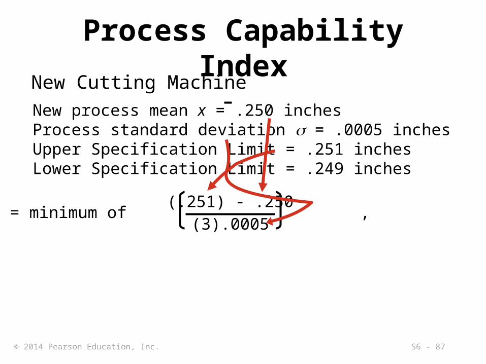
Process Capability IndexNew Cutting Machine
New process mean x = .250 inchesProcess standard deviation = .0005 inchesUpper Specification Limit = .251 inchesLower Specification Limit = .249 inches
© 2014 Pearson Education, Inc. S6 - 87
Process Capability IndexNew Cutting Machine
New process mean x = .250 inchesProcess standard deviation = .0005 inchesUpper Specification Limit = .251 inchesLower Specification Limit = .249 inches
Cpk = minimum of ,(.251) - .250
(3).0005
© 2014 Pearson Education, Inc. S6 - 88
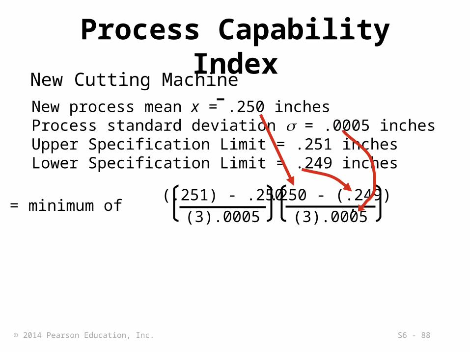
Process Capability IndexNew Cutting Machine
New process mean x = .250 inchesProcess standard deviation = .0005 inchesUpper Specification Limit = .251 inchesLower Specification Limit = .249 inches
Cpk = minimum of ,(.251) - .250
(3).0005.250 - (.249)
(3).0005

© 2014 Pearson Education, Inc. S6 - 89
Process Capability IndexNew Cutting Machine
New process mean x = .250 inchesProcess standard deviation = .0005 inchesUpper Specification Limit = .251 inchesLower Specification Limit = .249 inches
Cpk = = 0.67.001
.0015New machine is
NOT capable
Cpk = minimum of ,(.251) - .250
(3).0005.250 - (.249)
(3).0005
Both calculations result in

© 2014 Pearson Education, Inc. S6 - 90
Lower specification
limit
Upper specification
limit
Interpreting Cpk
Cpk = negative number (Process
does not meet specifications)
Cpk = zero (Process
does not meet specifications)
Cpk = between 0 and 1(Process
does not meet specifications)Cpk = 1 (Process meets
Specifications)
Cpk > 1 (Process meets
Specifications)
Figure S6.8

© 2014 Pearson Education, Inc. S6 - 91
Acceptance Sampling► Form of quality testing used for incoming
materials or finished goods► Take samples at random from a lot
(shipment) of items► Inspect each of the items in the sample► Decide whether to reject the whole lot
based on the inspection results► Only screens lots; does not drive quality
improvement efforts
© 2014 Pearson Education, Inc. S6 - 92
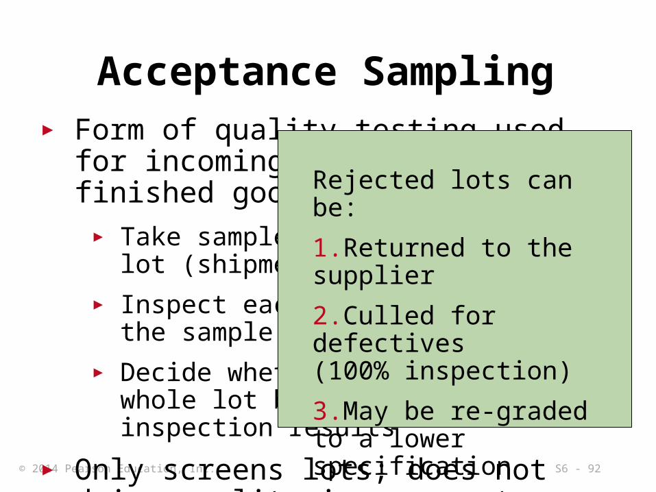
Acceptance Sampling► Form of quality testing used for incoming
materials or finished goods► Take samples at random from a lot
(shipment) of items► Inspect each of the items in the sample► Decide whether to reject the whole lot
based on the inspection results► Only screens lots; does not drive quality
improvement efforts
Rejected lots can be:1.Returned to the supplier2.Culled for defectives (100% inspection)3.May be re-graded to a lower specification

© 2014 Pearson Education, Inc. S6 - 93
Operating Characteristic Curve
► Shows how well a sampling plan discriminates between good and bad lots (shipments)
► Shows the relationship between the probability of accepting a lot and its quality level

© 2014 Pearson Education, Inc. S6 - 94
Return whole shipment
The “Perfect” OC Curve
% Defective in Lot
P(A
ccep
t Who
le S
hipm
ent)
100 –
75 –
50 –
25 –
0 –| | | | | | | | | | |
0 10 20 30 40 50 60 70 80 90 100
Cut-Off
Keep whole shipment

© 2014 Pearson Education, Inc. S6 - 95
An OC Curve
Probability of Acceptance
Percent defective
| | | | | | | | |0 1 2 3 4 5 6 7 8
= 0.05 producer’s risk for AQL
= 0.10
Consumer’s risk for LTPD
LTPDAQLBad lotsIndifference
zoneGood lots
Figure S6.9

© 2014 Pearson Education, Inc. S6 - 96
AQL and LTPD► Acceptable Quality Level (AQL)
► Poorest level of quality we are willing to accept
► Lot Tolerance Percent Defective (LTPD)► Quality level we consider bad► Consumer (buyer) does not want to accept
lots with more defects than LTPD
The probability of rejecting a good lot is called a type I error. The probability of accepting a bad lot is a type II error.

© 2014 Pearson Education, Inc. S6 - 97
Producer’s and Consumer’s Risks
► Producer's risk ()► Probability of rejecting a good lot ► Probability of rejecting a lot when the
fraction defective is at or above the AQL► Consumer's risk ()
► Probability of accepting a bad lot ► Probability of accepting a lot when
fraction defective is below the LTPD
© 2014 Pearson Education, Inc. S6 - 98
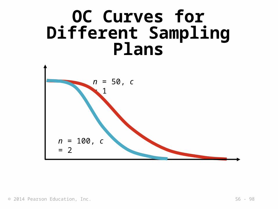
OC Curves for Different Sampling Plans
n = 50, c = 1
n = 100, c = 2

© 2014 Pearson Education, Inc. S6 - 99
Average Outgoing Quality
where
Pd = true percent defective of the lot
Pa = probability of accepting the lot
N = number of items in the lotn = number of items in the sample
AOQ = (Pd)(Pa)(N – n)
N

© 2014 Pearson Education, Inc. S6 - 100
Average Outgoing Quality1. If a sampling plan replaces all defectives2. If we know the incoming percent defective
for the lot
We can compute the average outgoing quality (AOQ) in percent defective
The maximum AOQ is the highest percent defective or the lowest average quality and is called the average outgoing quality limit (AOQL)

© 2014 Pearson Education, Inc. S6 - 101
Automated Inspection► Modern
technologies allow virtually 100% inspection at minimal costs
► Not suitable for all situations

© 2014 Pearson Education, Inc. S6 - 102
SPC and Process Variability
(a) Acceptance sampling (Some bad units accepted; the “lot” is good or bad)
(b) Statistical process control (Keep the process “in control”)
(c) Cpk > 1 (Design a process that is in within specification)
Lower specification
limit
Upper specification
limit
Process mean, Figure S6.10
© 2014 Pearson Education, Inc. S6 - 103
Thank you