Lecture 2: Energy levels in metal complexes: ligand field theory, spin-orbit coupling, zero-field-splitting, magnetic susceptibility Ligand Field Theory The full rotation group of a sphere: R3 or SU2 The full rotation group of a sphere has an infinite number of elements. The symmetry operations of R3 are all rotations about all axes of the sphere. As an exercice you may demonstrate that 2 rotations C(φ) about 2 different arbitrary axes but of the same angle φ belong to the same class. Recall that any symmetry operations commutes with the hamiltonian of the system that you consider. Hence the wave function associated to each of the terms 2S+1Γ of the free ion are a basis of the irreducible representations of the full rotation group R3 of a sphere. Indeed, a simple formula to determine the characters of a rotation by an angle Φ spanned through the 2l+1 functions |l ml> is easily obtained (exercice). Consider: |l,m> = F(r)Plm(θ)eimφ where R(Φ) is a rotation by an angle Φ about the polar axis; we thus obtain:

R(Φ)|l,m> = R(Φ)F(r)Plm(θ)eimφ = F(r)Plm(θ)eim(φ+Φ), m=-l,...,0,...,l. It is easily seen that the following diagonal matrix of dimension (2l+1) permits to represent R(Φ) :

! R " =

eil" 0

...

0 e-il"

and that the characters of this representation becomes

! " = eil" + ei l-1 " + ... + e-il" =

sin l+1

2"

sin "

2

If one generalizes for the case of many-electron functions, each irreducible representation Γ has as basis the 2L+1 spatial functions |L,ML> i.e. Γ=S if L=0, Γ=P if L=1, Γ=D if L=2, Γ=F if L=3, Γ=G if L=4, Γ=H if L=5, etc. .... Thus, the character associated to the rotation C(φ) is:

! " =

sin L+1

2"

sin "

2

The characters of the full rotation group R3 pour has the identity element E=C(0) and the operations of the class C(φ) are represented by:

R3 E ∞ C(φ) Γ

2L+1

sin L+1

2!

sin !

2

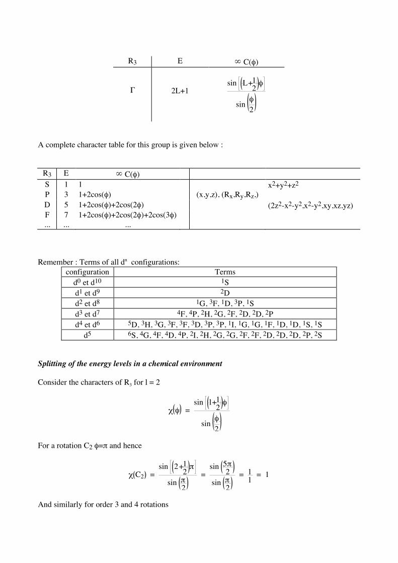
A complete character table for this group is given below :

R3 E ∞ C(φ) S 1 1 x2+y2+z2 P 3 1+2cos(φ) (x,y,z), (Rx,Ry,Rz,) D 5 1+2cos(φ)+2cos(2φ) (2z2-x2-y2,x2-y2,xy,xz,yz) F 7 1+2cos(φ)+2cos(2φ)+2cos(3φ) ... ... ...

Remember : Terms of all dn configurations:

configuration Terms d0 et d10 1S d1 et d9 2D d2 et d8 1G, 3F, 1D, 3P, 1S d3 et d7 4F, 4P, 2H, 2G, 2F, 2D, 2D, 2P d4 et d6 5D, 3H, 3G, 3F, 3F, 3D, 3P, 3P, 1I, 1G, 1G, 1F, 1D, 1D, 1S, 1S

d5 6S, 4G, 4F, 4D, 4P, 2I, 2H, 2G, 2G, 2F, 2F, 2D, 2D, 2D, 2P, 2S Splitting of the energy levels in a chemical environment Consider the characters of R3 for l = 2

! " =

sin l+1

2"

sin "

2

For a rotation C2 φ=π and hence

! C2 =

sin 2+1

2"

sin "2

=

sin 5"2

sin "2

= 1

1 = 1

And similarly for order 3 and 4 rotations

! C3 =

sin 2+1

2 2"

3

sin 1

2 2"

3

=

sin 5"3

sin "3

=

-sin "3

sin "3

= -1

! C4 =

sin 2+1

2 "2

sin "4

=

sin 5"4

sin "4

= -1

The formula is also valid for the case where φ=0 i.e.

χ(E) = 2l+1 = 5 This result can be obtained as follows, that is consider :

!

" # = 0( ) =lim

# $ 0

sin l +1 2( ) % #[ ]sin # 2( )

=l +1 2( ) % ## 2

= 2 % l +1 2( ) = 2l +1

In an octahedral (O symmetry point group) environment, using a character table e.g. : P.W. Atkins, M.S. Child, and C.S.P. Phillips; "Tables for Group Theory"; Oxford University Press 1970; the irrep d (l=2) is reducible and the reduction of irrep (short notation for irreducible representations) d (Tables for Group Theory cited above p. 24) yields e + t2. Consider a few typical examples: Example 1: Splitting of the |L ML> levels in an octahedral environment

Symmetyof level

L

χ(E)

χ(C2)

χ(C3)

χ(C4)

Irreducible representations

S 0 1 1 1 1 A1g P 1 3 -1 0 1 T1u D 2 5 1 -1 -1 Eg+T2g F 3 7 -1 1 -1 A2u+T1u+T2u G 4 9 1 0 1 A1g+Eg+T1g+T2g H 5 11 -1 -1 1 Eu+2T1u+T2u I 6 13 1 1 -1 A1g+A2g+Eg+T1g+2T2g

Example 2: Splitting of the d-orbitals in various symmetries

R3 Oh Td D4h D3 D2d

d

eg+t2g

e+t2

a1g+b1g+b2g+eg

a1+2e

a1+b1+b2+e Example 3: Splitting of all d2 terms in an octahedral environment There are two procedures. 1st procedure: weak field approach, the terms of the free ion are split by a weak chemical

environment (filed) 1G ! 1A1+1E+1T1+1T2 3F ! 3A2+3T1+3T2 1D ! 1E+1T2 3P ! 3T1 1S ! 1A1 2nd procedure: strong field approach, the d-orbitals are first split by a strong chemical environment (field) in eg et t2g and the inter-electronic repulsion acts as a perturbation. We shall consider all configurations egxt2gn-x (x = 0, 1, ..., n) and determine though the direct product all states stemming from each of those configurations. Our example yields eg2: eg ! eg = A1g + [A2g] + Eg ! 1A1g + 3A2g + 1Eg t2geg: t2g ! eg = T1g + T2g ! 1T1g + 3T1g + 1T2g+ 3T2g t2g2: t2g ! t2g = A1g + Eg + [T1g] + T2g ! 1A1g + 1Eg + 3T1g + 1T2g Both procedure are obviously equivalent as illustrated in the correlation diagram below:

Double Groups The relation

! " =

sin L+1

2"

sin "

2

was obtained neglecting the coupling between the orbital momentum

!

r L and the spin

!

r S . However, if

one does consider this coupling the resulting momentum

J = L + S has to be considered. The relation of χ(φ) for the functions associated to a (2J+1)-fold degenerate state reads

! " =

sin J +1

2"

sin "

2

where J is the quantum number associated to J. The possible values for L are all integers, whereas J can also take half integer values. Let’s now consider a rotation by an angle φ followed by a rotation of 2π about the same axis; if J is integer, the equation above becomes:

! "+2# = ! " However if J is half-integer we get :

! "+2# = -! " Hence a rotation of 2π can no longer be considered as the identity operation. However a rotation of 4π corresponds to the identity. To circumvent this difficulty, Bethe proposed note a rotation of 2π by R and to associate to each symmetry group G a new one labelled G* containing all elements of G plus the direct product R by G

!

G* = G,R"G{ }

Example 1: Irreducible representation spanned by a spin doublet:

!

"

Let’s apply the relation for χ(φ) with J=1/2, we get:

O*

E

R

4C3

4C3

2R

= 8C3

4C3R

4C3

2

= 8C3R

3C2

3C2R

= 6C2

3C4

3C4

3R

= 6C4

3C4R

3C4

3

= 6C4R

6C2

'

6C2

'R

= 12C2

'

!"

#

2

-2

1

-1

0

2

- 2

0

verifying in: P.W. Atkins, M.S. Child, and C.S.P. Phillips; "Tables for Group Theory"; Oxford University Press 1970, we notice:

!"

#

= E1/2

Example 2: Irreducible representation spanned by a spin doublet triplet J=1 is integer and yields:

Γtriplet = T1 Exemple 3: Determine all spin-orbit components for the ground state 3T1 of d2 ion in an octahedral ligand field: All we have to do is to get the direct product between the irrep of the space part i.e. T1 and the irrep of the spin part Γtriplet = T1. One obtains :

T1 ! T1 = A1 + E + T1 + T2 Hence, le term considered splits under the spin-orbit coupling according to the following scheme:

3T1 ! A1 + E + T1 + T2 Angular Overlap Model (AOM) and ligand field model a) Ligand field model We want to represent the action of the chemical environment through an electrostatic perturbation h = ho + vLF where ho is the hamiltonien of the free ion and vLF the electrostatic potential of ligand charge density at the metallic centre. If ρ(r) the charge density due to the ligands one obtains for the electrostatic potential

v(r) = -e !(R)

R - r dR

The symbols used are defined in the fig. below an e represents the charge of the electron.

L

L

L

M

r

R!

Expand 1/|r-R| to obtain

1

R - r = 1

r<

r<

r>

k

!k=0

!

Pk cos "

where r< = min{r,R}, r> = max{r,R} and Pk(x) is a Legendre polynomial of order k. We suppose (van Vleck and Bethe, 1928) that

r < R With this hypothesis, we get:

1

R - r = 1

R r

R

k!k=0

!

Pk cos "

Moreover the Legendre polynomial may be expressed in term of spherical harmonics Ykm:

Pk cos ! = 4"2k+1

Ykm!m=-k

+k

(#,$ ) Ykm* (%,&)

where r = (r,θ,φ) and R = (R,Θ,Φ). Thus, one obtains:

vLF = hkq!q=-k

+k

!k=0

2l

Ykq

l=2 for d-electrons and =3 for f-electrons; the parameters hkq are adjustable and describe the ligand field. The two following relation are useful:

hkq = - 4!e2k+1

<rk> "(R) Ykq

* (#,$)

RK+1 dR

= (-1)m (2k+1) l l k-m m' q

<lm|vLF|lm'>!m,m'

!

j1 j2 j3

m1 m2 m3

"

# $

%

& ' are the well-known 3-j symbols of Wigner. The matrix <lm|vLF|lm'> has the

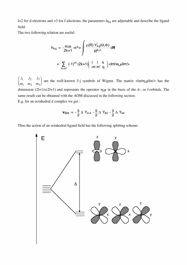
dimension (2l+1)x(2l+1) and represents the operator vLF in the basis of the d-, or f-orbitals. The same result can be obtained with the AOM discussed in the following section. E.g. for an octahedral d complex we get :

vOh = - 3

2 ! Y4-4 - 5

2 ! Y40 - 3

2 ! Y44

Thus the action of an octahedral ligand field has the following splitting scheme:

E z

x

y

x

zz

yx

y

!

b) Angular Overlap Model (AOM) Consider:

-e !

!L

dz2

e!

z

Consider now other possible types of M-L interactions: no nodal plane: σ one nodal plane: π two nodal planes: δ (never observed)

z

z

Définition de e!Définition de e"

Consider the splitting of the 5 d-orbitals due to a local M-L interaction:

(xy, x2-y2)

(xz, yz)

(z2)

|nd>

e!

e"

A semi-quantitative physical interpretation of the parameters eσ et eπ can be estimated as follows:

ek ! <"M|h|"Lk

>2

<"M|h|"M> - <"Lk|h|"Lk

> ! const. <"M|"L>

2

where h is an effective hamiltonian for the M-L entity and ψ represents respectively the orbitals of the metal M and of the ligand L, i.e. σ or π. If we suppose additivity and transferability of the AOM parameters we obtain for the ligand field

v = vL!L

The calculation of the elements <di|v|dj> in the basis of d-orbitals: d1 = dz2 = R(r) (3z2-r2)/(2√3) d2 = dyz = R(r) yz d3 = dxz = R(r) xz d4 = dxy = R(r) xy d5 = dx2-y2 = R(r) (x2-y2)/2 is illustrated below. Let us first consider the interaction of a ligand L in axial z position with the d-orbitals , i.e. <di|vzL|dj> = vzij,L

vzL z2 yz xz xy x2-y2 z2 σL yz πL xz πL xy 0

x2-y2 0 Next consider the interaction of ligand L on the x-axis with the d-orbitals, i.e. <di|vxL|dj> = vxij,L = ? . we have to carry out the following axis transformation:

x ! Z

y ! Y

z ! -X

and let us apply this transformation to the previous system

DZ2dz2

Y=y

X

Zx

y

z

we obviously get

vLx = vL

Z and

dz2 ! 1

2 3 3z2 - r2 = 1

2 3 3X

2 - R

2 =

- 1

2 1

2 3 3Z

2 - R

2 + 3

2 1

2 X

2 - Y

2 =

- 1

2 DZ

2 + 3

2 DX

2-Y

2

Hence

< dz2 | vLx | dz2 > = < - 1

2 DZ

2 + 3

2 DX

2-Y

2 | vLZ | - 1

2 DZ

2 + 3

2 DX

2-Y

2 > =

1

4 < DZ

2 | vLZ | DZ

2 > - 3

4 < DZ

2 | vLZ | DX

2-Y

2 > - 3

4 < DX

2-Y

2 | vLZ | DZ

2 > + 3

4 < DX

2-Y

2 | vLZ | DX

2-Y

2 >

= 1

4 < DZ

2 | vLZ | DZ

2 > = 1

4 !L

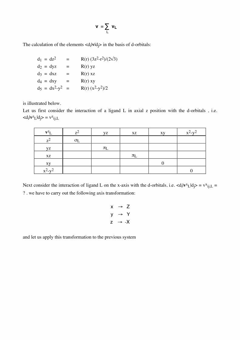
If we apply the same calculation to all elements <di|vxL|dj> = vxij,L we get

vxL z2 yz xz xy x2-y2 z2 1

4 !L - 3

4 !L

yz xz πL xy πL

X2-y2 - 3

4 !L 1

4 !L

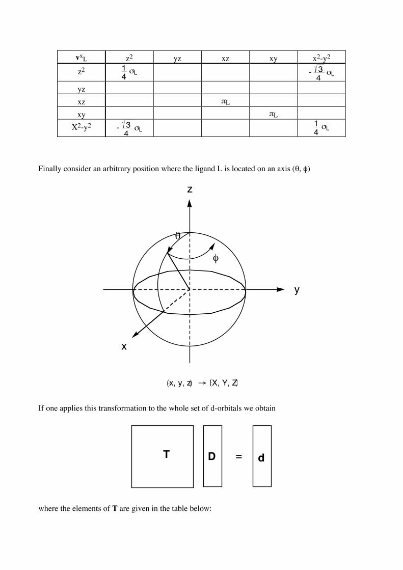
Finally consider an arbitrary position where the ligand L is located on an axis (θ, φ)

x

y

z

!

"

x, y, z ! X, Y, Z If one applies this transformation to the whole set of d-orbitals we obtain

dDT =

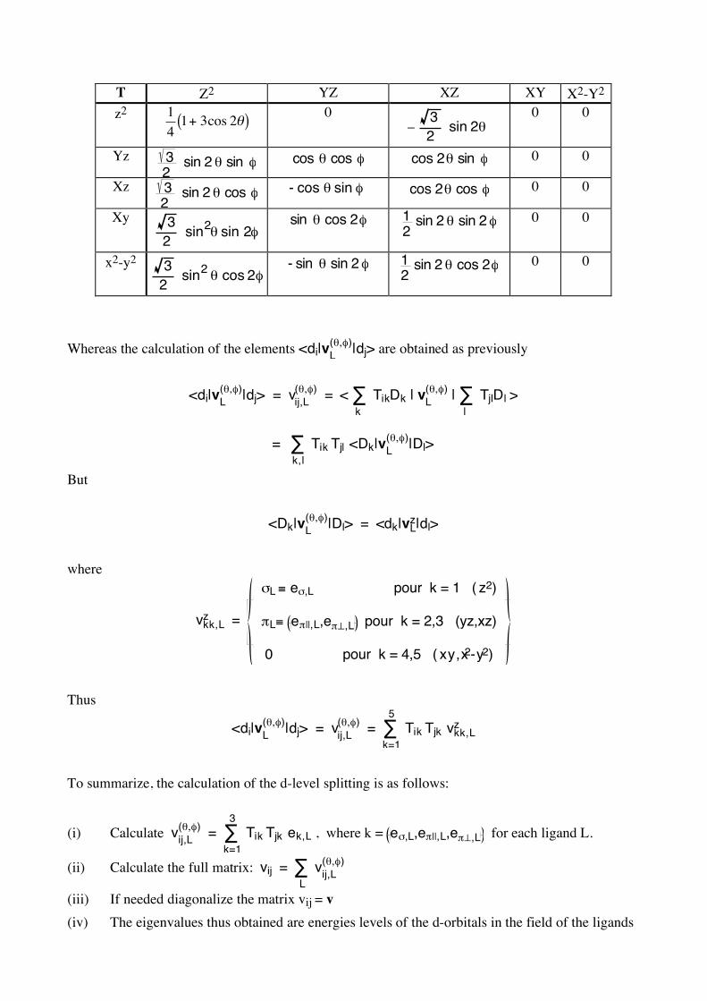
where the elements of T are given in the table below:

T Z2 YZ XZ XY X2-Y2 z2

!

1

41+ 3cos 2"( ) 0

–3

2sin 2!

0 0

Yz 3

2 sin 2 ! sin " cos ! cos " cos 2! sin " 0 0

Xz 3

2 sin 2 ! cos " - cos ! sin " cos 2! cos " 0 0

Xy 3

2sin

2! sin 2"

sin ! cos 2" 1

2 sin 2 ! sin 2 " 0 0

x2-y2 3

2sin

2! cos 2"

- sin ! sin 2 " 1

2 sin 2 ! cos 2" 0 0

Whereas the calculation of the elements <di|vL

(!,")|dj> are obtained as previously

<di|vL

(!,")|dj> = v

ij,L

(!,") = < TikDk !

k

| vL

(!,") | TjlDl !

l

>

= !k,l

Tik Tjl <Dk|vL

(!,")|Dl>

But

<Dk|vL

(!,")|Dl> = <dk|vL

z|dl>

where

vkk,Lz =

!L " e!,L pour k = 1 ( z2)

#L" e#||,L,e#$,L pour k = 2,3 (yz,xz)

0 pour k = 4,5 ( xy,x2-y2)

Thus

<di|vL

(!,")|dj> = v

ij,L

(!,") = Tik Tjk vkk,L

z!k=1

5

To summarize, the calculation of the d-level splitting is as follows:

(i) Calculate vij,L

(!,") = Tik Tjk ek,L!

k=1

3

, where k = e!,L,e"||,L,e"#,L for each ligand L.

(ii) Calculate the full matrix: vij = vij,L

(!,")!L

(iii) If needed diagonalize the matrix vij = v (iv) The eigenvalues thus obtained are energies levels of the d-orbitals in the field of the ligands

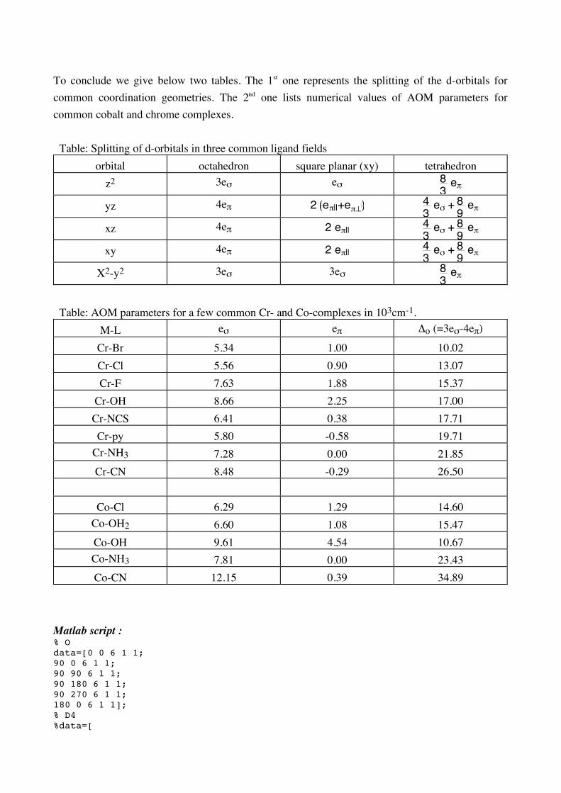
To conclude we give below two tables. The 1st one represents the splitting of the d-orbitals for common coordination geometries. The 2nd one lists numerical values of AOM parameters for common cobalt and chrome complexes. Table: Splitting of d-orbitals in three common ligand fields

orbital octahedron square planar (xy) tetrahedron z2 3eσ eσ 8

3 e!

yz 4eπ 2 e!||+e!" 4

3 e! + 8

9 e"

xz 4eπ 2 e!|| 4

3 e! + 8

9 e"

xy 4eπ 2 e!|| 4

3 e! + 8

9 e"

X2-y2 3eσ 3eσ 8

3 e!

Table: AOM parameters for a few common Cr- and Co-complexes in 103cm-1.

M-L eσ eπ Δo (=3eσ-4eπ)

Cr-Br 5.34 1.00 10.02 Cr-Cl 5.56 0.90 13.07 Cr-F 7.63 1.88 15.37

Cr-OH 8.66 2.25 17.00 Cr-NCS 6.41 0.38 17.71 Cr-py 5.80 -0.58 19.71

Cr-NH3 7.28 0.00 21.85 Cr-CN 8.48 -0.29 26.50

Co-Cl 6.29 1.29 14.60

Co-OH2 6.60 1.08 15.47 Co-OH 9.61 4.54 10.67 Co-NH3 7.81 0.00 23.43 Co-CN 12.15 0.39 34.89

Matlab script : % O data=[0 0 6 1 1; 90 0 6 1 1; 90 90 6 1 1; 90 180 6 1 1; 90 270 6 1 1; 180 0 6 1 1]; % D4 %data=[

%90 0 6 1 1; %90 90 6 1 1; %90 180 6 1 1; %90 270 6 1 1]; % D3 %data=[ 54.7356 0 1. .0 .0; % 54.7356 120 1. .0 .0; % 54.7356 240 1. .0 .0; % 125.2644 60 1. .0 .0; % 125.2644 180 1. .0 .0; % 125.2644 300 1. .0 .0]; % Icosahedron %data=[ % 0 0 1 0.1 0.1; % 63.4349 90.0000 1 0.1 0.1; % 63.4349 18.0000 1 0.1 0.1; % 63.4349 306.0000 1 0.1 0.1; % 63.4349 234.0000 1 0.1 0.1; % 63.4349 162.0000 1 0.1 0.1; % 116.5651 270.0000 1 0.1 0.1; % 116.5651 198.0000 1 0.1 0.1; % 116.5651 126.0000 1 0.1 0.1; % 116.5651 54.0000 1 0.1 0.1; % 116.5651 342.0000 1 0.1 0.1; % 180.0000 0 1 0.1 0.1]; n=size(data);conv=pi/180; for i=1:5 for j=1:5 v(i,j)=0; for l=1:n(1) t=trd(conv*data(l,1:2)); for k=1:3 v(i,j)=v(i,j)+t(i,k)*t(j,k)*data(l,k+2); end end end end disp(' Dsigma Dpi,s Dpi,c Ddel,s Ddel,c') disp(v) [c e]=eig(v); [e iv]=sort(diag(e)); e=e';disp(' ');disp(e) c=c(:,iv);disp(c) %v %[c e]=eig(v); %[e iv]=sort(diag(e)); %e=e' %c=c(:,iv) function t=trd(w) theta=w(1);phi=w(2); sq=sin(theta);cq=cos(theta);s2q=sin(theta+theta); c2q=cos(theta+theta);sq2=sq*sq; sf=sin(phi);cf=cos(phi);s2f=sin(phi+phi);c2f=cos(phi+phi); r32=0.5*sqrt(3); t=[0.25*(1+3*c2q) 0 -r32*s2q; r32*s2q*sf cq*cf c2q*sf; r32*s2q*cf -cq*sf c2q*cf; r32*sq2*s2f sq*c2f 0.5*s2q*s2f; r32*sq2*c2f -sq*s2f 0.5*s2q*c2f];

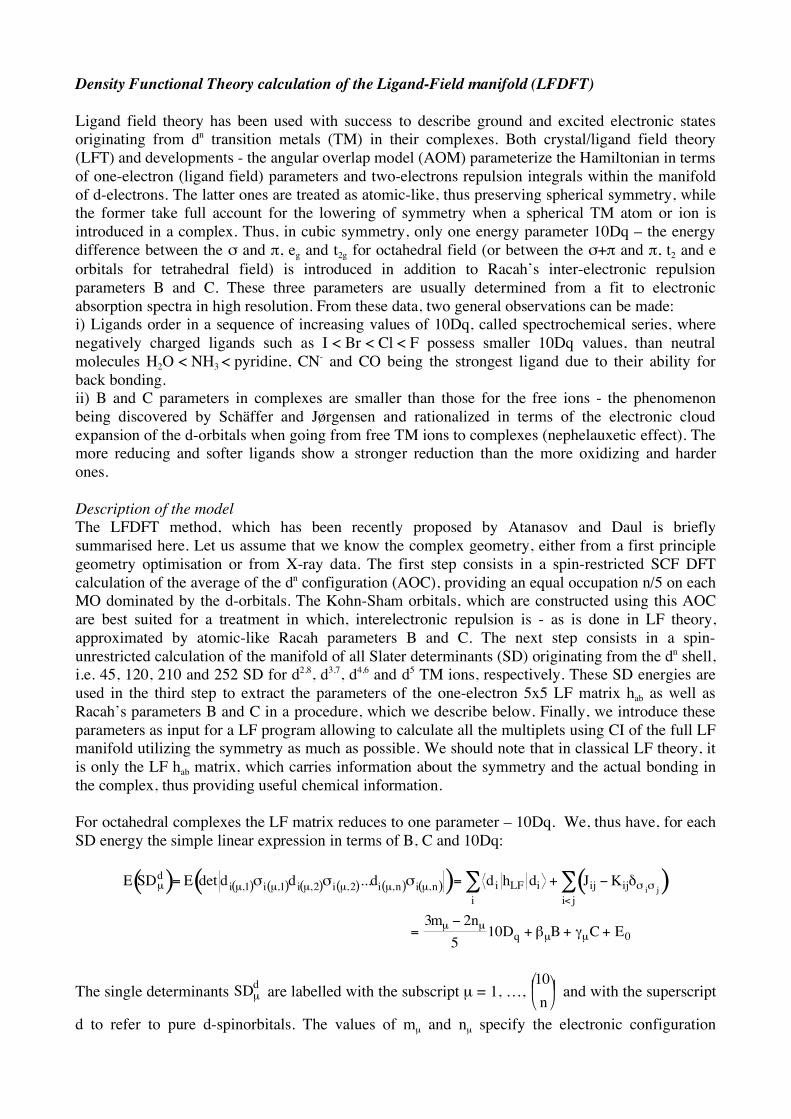
Density Functional Theory calculation of the Ligand-Field manifold (LFDFT) Ligand field theory has been used with success to describe ground and excited electronic states originating from dn transition metals (TM) in their complexes. Both crystal/ligand field theory (LFT) and developments - the angular overlap model (AOM) parameterize the Hamiltonian in terms of one-electron (ligand field) parameters and two-electrons repulsion integrals within the manifold of d-electrons. The latter ones are treated as atomic-like, thus preserving spherical symmetry, while the former take full account for the lowering of symmetry when a spherical TM atom or ion is introduced in a complex. Thus, in cubic symmetry, only one energy parameter 10Dq – the energy difference between the σ and π, eg and t2g for octahedral field (or between the σ+π and π, t2 and e orbitals for tetrahedral field) is introduced in addition to Racah’s inter-electronic repulsion parameters B and C. These three parameters are usually determined from a fit to electronic absorption spectra in high resolution. From these data, two general observations can be made: i) Ligands order in a sequence of increasing values of 10Dq, called spectrochemical series, where negatively charged ligands such as I < Br < Cl < F possess smaller 10Dq values, than neutral molecules H2O < NH3 < pyridine, CN- and CO being the strongest ligand due to their ability for back bonding. ii) B and C parameters in complexes are smaller than those for the free ions - the phenomenon being discovered by Schäffer and Jørgensen and rationalized in terms of the electronic cloud expansion of the d-orbitals when going from free TM ions to complexes (nephelauxetic effect). The more reducing and softer ligands show a stronger reduction than the more oxidizing and harder ones. Description of the model The LFDFT method, which has been recently proposed by Atanasov and Daul is briefly summarised here. Let us assume that we know the complex geometry, either from a first principle geometry optimisation or from X-ray data. The first step consists in a spin-restricted SCF DFT calculation of the average of the dn configuration (AOC), providing an equal occupation n/5 on each MO dominated by the d-orbitals. The Kohn-Sham orbitals, which are constructed using this AOC are best suited for a treatment in which, interelectronic repulsion is - as is done in LF theory, approximated by atomic-like Racah parameters B and C. The next step consists in a spin-unrestricted calculation of the manifold of all Slater determinants (SD) originating from the dn shell, i.e. 45, 120, 210 and 252 SD for d2,8, d3,7, d4,6 and d5 TM ions, respectively. These SD energies are used in the third step to extract the parameters of the one-electron 5x5 LF matrix hab as well as Racah’s parameters B and C in a procedure, which we describe below. Finally, we introduce these parameters as input for a LF program allowing to calculate all the multiplets using CI of the full LF manifold utilizing the symmetry as much as possible. We should note that in classical LF theory, it is only the LF hab matrix, which carries information about the symmetry and the actual bonding in the complex, thus providing useful chemical information. For octahedral complexes the LF matrix reduces to one parameter – 10Dq. We, thus have, for each SD energy the simple linear expression in terms of B, C and 10Dq:

!

E SDµd( )= E det di µ,1( )" i µ,1( )di µ,2( )" i µ,2( )...di µ,n( )" i µ,n( )( )= di hLF di

i

# + Jij $Kij%" i" j( )i< j

#

=3mµ $ 2nµ

510Dq + &µB + 'µC + E0

The single determinants

!

SDµd are labelled with the subscript µ = 1, …,

!

10

n

"

# $ %

& ' and with the superscript

d to refer to pure d-spinorbitals. The values of mµ and nµ specify the electronic configuration

µµ m

g

n

2g et , while the βµ and γµ are coefficients obtained after substituting standard expressions for the Coulomb Jij and exchange Kij integrals in terms of d-only orbitals di and spin functions σi. E0 represents the gauge origin of energy. Having obtained energy expressions for each

!

SDµd : 10Dq, B, C and E0 are estimated using a least-

squares procedure. Using matrix notation, we thus obtain an overdetermined system of linear equations with the unknown parameters stored in X and given below.

XAE = , i.e. EAA)AXT-1T(=

Comparing SD energies from DFT with those calculated using the LF parameter values, we can state for all considered cases, that the LF parameterization scheme is remarkably compatible with SD energies from DFT; standard deviations between DFT-SD energies and their LFDFT values are generally between 0.01 and 0.1 eV as shown in the Fig. Below.

This model can obviously be generalized allowing to treat systems with symmetry lower than cubic or even without any symmetry (C1). Here we make use of the general observation that the KS orbitals and the set of SD considered in eq.(1) convey all the information needed to setup the LF matrix. Following the effective Hamiltonian approach, let us consider the KS orbitals dominated by d-functions which result from an AOC dn DFT-SCF calculation. From the components of the eigenvector matrix built up from such MOs one takes only the components corresponding to the d functions. Let us denote the square matrix composed of the new column vectors by U and introduce the overlap matrix S:

S = UUT Since U is in general not orthogonal, we use Löwdin’s symmetric orthogonalisation procedure to obtain an equivalent set of orthogonal eigenvectors (C):

!

C = S"1

2U We identify now these vectors as the eigenfunctions of the effective LF Hamiltonian

!

hLFeff sought, as

!

" i = cµidµ

µ=1

5

#

Thus, the fitting procedure described in the previous section will enable us to estimate

!

hii = " i hLFeff

" i and hence the full representation matrix of

!

hLFeff as

!

hµ" = dµ hLFeffd" = cµihiic"i

i=1

5

#

The next step is now to generalize the fitting procedure for the case of no or low symmetry. The energy of a single determinant becomes thus:

!

E SDk"( )= E det " i k,1( )# i k,1( )" i k,2( )# i k,2( )..." i k,n( )# i k,n( )( )= " i hLF " i

i

$ + J ij %Kij&#i# j( )i< j

$

Where

!

SDk

" is composed of the spinorbitals mentioned earlier. In order to calculate the electrostatic contribution, it is useful to consider the transformation from the basis of

!

SDk

" to the one of

!

SDµd . Using basic linear algebra, we get:

!

SDk

"= Tkµ SDµ

d

µ

#

Where

!

Tkµ = detci k,1:n( ), j µ,1:n( ) i.e. the determinant of a nxn sub-matrix of

!

C" #

!

ci k,1( ), j µ ,1( ) ci k,1( ), j µ ,2( ) ... ci k,1:n( ), j µ,n( )

ci k,2( ), j µ,1( ) ci k,2( ), j µ,2( ) ... ci k,2( ), j µ,n( )

... ... ... ...

ci k,n( ), j µ,1( ) ci k,n( ), j µ,2( ) ... ci k,n( ), j µ,n( )

With the indices of the spinorbitals

!

" i k,1( )# i k,1( )," i k,2( )# i k,2( ), ...," i k,n( )# i k,n( ) and

!

dj µ ,1( )" j µ,1( ), dj µ,2( )" j µ ,2( ), ..., dj µ ,n( )" j µ,n( ) respectively. Note that these indices are in fact a two-dimensional array of (number of SD) x (number of electrons or holes) integers. Finally the energy of a SD can be rewritten as

!

Ek = E SDk

"( )= " i hLF " ii

# + TkµTk$ SDµdG SD$

d

µ ,$

#

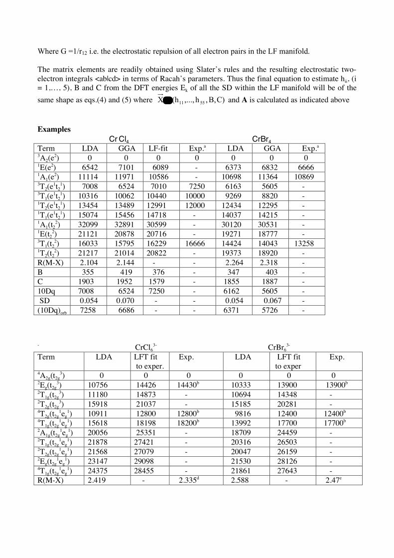
Where G =1/r12 i.e. the electrostatic repulsion of all electron pairs in the LF manifold. The matrix elements are readily obtained using Slater’s rules and the resulting electrostatic two-electron integrals <ab|cd> in terms of Racah’s parameters. Thus the final equation to estimate hii, (i = 1,…, 5), B and C from the DFT energies Ek of all the SD within the LF manifold will be of the same shape as eqs.(4) and (5) where C)B,,h,...,(hX 5511= and A is calculated as indicated above Examples

Cr Cl4 CrBr4 Term LDA GGA LF-fit Exp.a LDA GGA Exp.a 3A2(e2) 0 0 0 0 0 0 0 1E(e2) 6542 7101 6089 - 6373 6832 6666 1A1(e2) 11114 11971 10586 - 10698 11364 10869 3T2(e1t2

1) 7008 6524 7010 7250 6163 5605 - 3T1(e1t2

1) 10316 10062 10440 10000 9269 8820 - 1T2(e1t2

1) 13454 13489 12991 12000 12434 12295 - 1T1(e1t2

1) 15074 15456 14718 - 14037 14215 - 1A1(t2

2) 32099 32891 30599 - 30120 30531 - 1E(t2

2) 21121 20878 20716 - 19271 18777 - 3T1(t2

2) 16033 15795 16229 16666 14424 14043 13258 1T2(t2

2) 21217 21014 20822 - 19373 18920 - R(M-X) 2.104 2.144 - - 2.264 2.318 - B 355 419 376 - 347 403 - C 1903 1952 1579 - 1855 1887 - 10Dq 7008 6524 7250 - 6162 5605 - SD 0.054 0.070 - - 0.054 0.067 - (10Dq)orb 7258 6686 - - 6371 5726 - - CrCl6

3- CrBr63-

Term LDA LFT fit to exper.

Exp. LDA LFT fit to exper

Exp.

4A2g(t2g3) 0 0 0 0 0 0

2Eg(t2g3) 10756 14426 14430b 10333 13900 13900b

2T1g(t2g3) 11180 14873 - 10694 14348 -

2T2g(t2g3) 15918 21037 - 15185 20281 -

4T2g(t2g1eg

1) 10911 12800 12800b 9816 12400 12400b 4T1g(t2g

1eg1) 15618 18198 18200b 13992 17700 17700b

2A1g(t2g1eg

1) 20056 25351 - 18709 24459 - 2T1g(t2g

1eg1) 21878 27421 - 20316 26503 -

2T2g(t2g1eg

1) 21568 27079 - 20047 26159 - 2Eg(t2g

1eg1) 23147 29098 - 21530 28126 -

4T1g(t2g1eg

1) 24375 28455 - 21861 27643 - R(M-X) 2.419 - 2.335d 2.588 - 2.47e

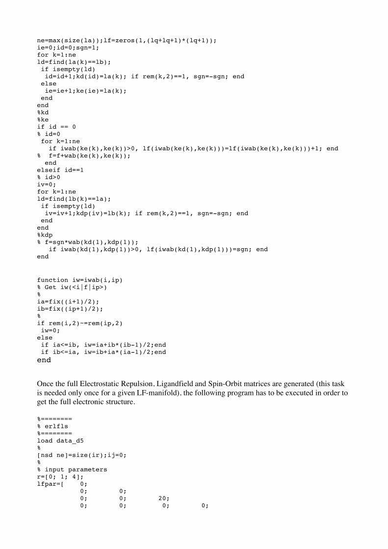
Practical calculation of energy levels in metal complexes: Multiplets, Spin-Orbit and Zero-Field-Splitting The calculation of energy levels within the whole ligand field manifold is now an easy task. All we need is to combine the results of the previous chapters. This, is best achieved using computational methods in the MATLAB environment. The Matlab script below is an extension to the ones presented in Chap. 2. This procedure calls :

(i) get2ei4a : gets all 2-electron integrals for atoms with open [lq(1) lq(2) …]Ne-shells. The the electrostatic matrixelements <iabcd( :,1) iabcd( :,2) | iabcd( :,3) iabcd( :,4) > = vabcd(:,:)*parameters(:). The target transformation following the call to get2ei4a re-expresses the abstract Slater-Condon parameters into non-redundant <ab|cd>.

(ii) genersd : generates all single determinants for n electrons occupying spinorbitals k_start to k_end.

(iii) getls : get l, s and l.s one-electron matrices % % generate g-, lf-, ls-data for lq^ne % %global iabcd vabcd % global lq % global lx ly lz sx sy sz ls % % get - electrostatic 2-electron matrix elements % - ligandfield 1-electron matrix elements % - spin and orbit 1-electron matrix elements t0=cputime; %lq=[2,0]; lq=[3]; ne=1; % % generate single determinants or microstates for lq^ne ir=genersd(ne,1,2*sum(lq+lq+1)); % % get <ab|cd> %[vabcd,iabcd]=get2ei4a(lq); % % get l, s and l*s 1-e matrices: l=2 & s=1/2 [lx,ly,lz,sx,sy,sz,ls]=getls(lq,1/2); % % calculate nsd=length(ir);ij=0; for i=1:nsd for j=1:i ij=ij+1; lfdata(ij,:)=lfab(ir(i,:),ir(j,:)); lsdata(ij,:)=zab(ir(i,:),ir(j,:)); % gdata(ij,:)=gab(ne,ir(i,:),ir(j,:)); end end Elapsed_time=cputime-t0 %save data_d2 ir gdata lfdata lsdata save data_f1 ir lfdata lsdata function lf=lfab(la,lb) global lq; % Get <A|lf(1:(lq+lq+1)*(lq+1))|jB> %

ne=max(size(la));lf=zeros(1,(lq+lq+1)*(lq+1)); ie=0;id=0;sgn=1; for k=1:ne ld=find(la(k)==lb); if isempty(ld) id=id+1;kd(id)=la(k); if rem(k,2)==1, sgn=-sgn; end else ie=ie+1;ke(ie)=la(k); end end %kd %ke if id == 0 % id=0 for k=1:ne if iwab(ke(k),ke(k))>0, lf(iwab(ke(k),ke(k)))=lf(iwab(ke(k),ke(k)))+1; end % f=f+wab(ke(k),ke(k)); end elseif id==1 % id>0 iv=0; for k=1:ne ld=find(lb(k)==la); if isempty(ld) iv=iv+1;kdp(iv)=lb(k); if rem(k,2)==1, sgn=-sgn; end end end %kdp % f=sgn*wab(kd(1),kdp(1)); if iwab(kd(1),kdp(1))>0, lf(iwab(kd(1),kdp(1)))=sgn; end end function iw=iwab(i,ip) % Get iw(<i|f|ip>) % ia=fix((i+1)/2); ib=fix((ip+1)/2); % if rem(i,2)~=rem(ip,2) iw=0; else if ia<=ib, iw=ia+ib*(ib-1)/2;end if ib<=ia, iw=ib+ia*(ia-1)/2;end end Once the full Electrostatic Repulsion, Ligandfield and Spin-Orbit matrices are generated (this task is needed only once for a given LF-manifold), the following program has to be executed in order to get the full electronic structure. %======== % erlfls %======== load data_d5 % [nsd ne]=size(ir);ij=0; % % input parameters r=[0; 1; 4]; lfpar=[ 0; 0; 0; 0; 0; 20; 0; 0; 0; 0;

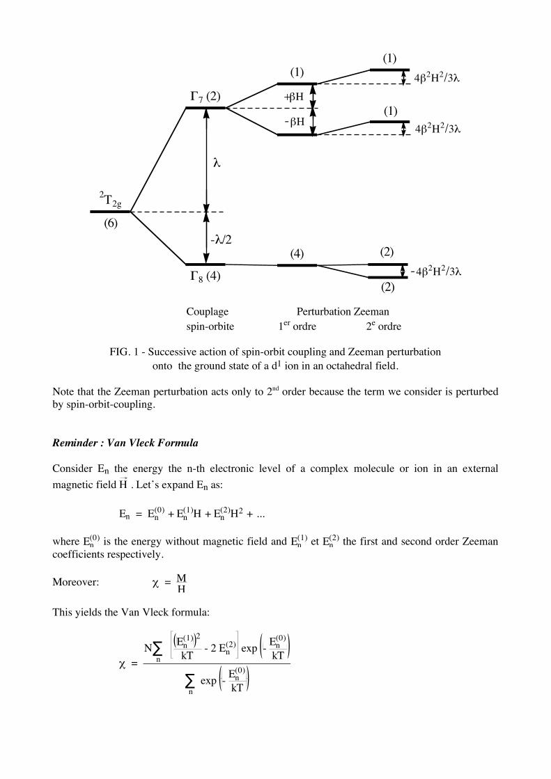
0; 0; 0; 0; 20]; zeta=0.2; % % get electrostatic matrix in basis of microstates ij=0; for i=1:nsd for j=1:i ij=ij+1; h(i,j)=gdata(ij,:)*r+lfdata(ij,:)*lfpar+lsdata(ij,7)*zeta; h(j,i)=conj(h(i,j)); end end % get Eigenvalues and Eigenvectors of h [c,e]=eig(h);[e,ie]=sort(real(diag(e))); e=e-e(1)*ones(size(e));c=c(:,ie); % sort according to multiplicities i0=1;i1=0; for i=2:nsd if abs(e(i)-e(i-1))>0.001 i1=i1+1;w(i1)=e(i-1);mul(i1)=i-i0;i0=i; end end i1=i1+1;w(i1)=e(i0);mul(i1)=nsd-i0+1; % print result fprintf('_____________________________ \n') fprintf(' Multiplicity E \n') fprintf('_____________________________ \n') for i=1:i1 fprintf(' %3i %12.3f\n',mul(i),w(i)) end fprintf('_____________________________ \n') Interaction of paramagnetic electrons in a metal complex with an external magnetic field. Example : Ground state of d1 Consider the ground state 2T2g of a d1 ion in an octahedral ligandfield. We suppose that the excited 2Eg state is sufficiently separated in energy from the ground state. If we neglect 2nd order spin-orbit coupling, the ground state 2T2g will split into a new ground state Γ8 that is fourfold degenerate and in a doublet Γ7 higher in energy by an amount of 3

2 !. Next, we consider the interaction with an

external magnetic field (Zeeman) to 1st order, i.e.

!

"82T2g( )

r H # $

r L + ge$

r S ( ) "8 2

T2g( ) . If we

diagonalize this matrix a surprising result is obtained, that is, the orbital contribution ! L" H compensates exactly the spin contribution !geS" H (if we take ge = 2). Thus, Γ8 is accidentally not influenced to 1st order by the Zeeman perturbation. However, Γ7 is split into two components by an amount ±!H versus Γ7. To second order the components of Γ7 and Γ8 couple. Two components of

Γ8 are lowered by - 4

3 !

2H2

", the two others remain unchanged. The components of Γ7 are both

destabilized by 4

3 !

2H2

". The whole splitting pattern is represented graphically in figure 1 below.

Note that this result is independent of the direction of the magnetic field since the complex is cubic and hence magnetically isotropic.

Couplage Perturbation Zeeman

spin-orbite 1er ordre 2e ordre

-4!2H2/3"

4!2H2/3"

4!2H2/3"

-!H

+!H

(2)

(2)(4)

(1)

(1)(1)

#8 (4)

#7 (2)

-"/2

"

(6)

2T2g

FIG. 1 - Successive action of spin-orbit coupling and Zeeman perturbation onto the ground state of a d1 ion in an octahedral field.

Note that the Zeeman perturbation acts only to 2nd order because the term we consider is perturbed by spin-orbit-coupling. Reminder : Van Vleck Formula Consider En the energy the n-th electronic level of a complex molecule or ion in an external magnetic field H . Let’s expand En as: En = En

(0) + En(1)H + En

(2)H2 + ... where En

(0) is the energy without magnetic field and En(1) et En

(2) the first and second order Zeeman coefficients respectively. Moreover: ! =

M

H

This yields the Van Vleck formula:

! =

N En

(1) 2

kT - 2 En

(2) exp - En

(0)

kT!n

exp - En

(0)

kT!n

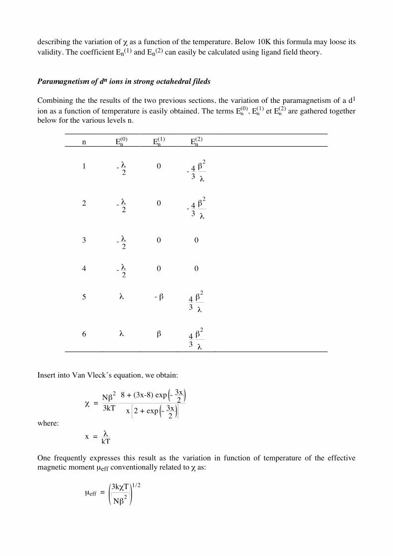
describing the variation of χ as a function of the temperature. Below 10K this formula may loose its validity. The coefficient En(1) and En(2) can easily be calculated using ligand field theory. Paramagnetism of dn ions in strong octahedral fileds Combining the the results of the two previous sections, the variation of the paramagnetism of a d1 ion as a function of temperature is easily obtained. The terms En

(0), En(1) et En

(2) are gathered together below for the various levels n.

n En(0) En

(1) En(2)

1

- !

2

0

- 4

3 !

2

"

2

- !

2

0

- 4

3 !

2

"

3

- !

2

0

0

4

- !

2

0

0

5

λ

- β

4

3 !

2

"

6

λ

β

4

3 !

2

"

Insert into Van Vleck’s equation, we obtain:

! = N"

2

3kT 8 + (3x-8) exp - 3x

2

x 2 + exp - 3x2

where: x = !

kT

One frequently expresses this result as the variation in function of temperature of the effective magnetic moment µeff conventionally related to χ as:

µeff = 3k!T

N"2

1/2

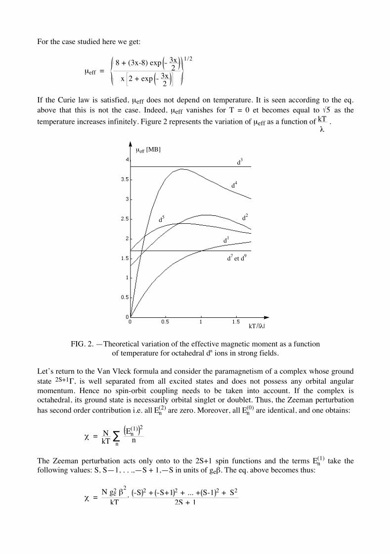
For the case studied here we get:

µeff = 8 + (3x-8) exp - 3x

2

x 2 + exp - 3x2

1/2

If the Curie law is satisfied, µeff does not depend on temperature. It is seen according to the eq. above that this is not the case. Indeed, µeff vanishes for T = 0 et becomes equal to 5 as the temperature increases infinitely. Figure 2 represents the variation of µeff as a function of kT

! .

kT/|!|

µeff [MB]

d5

d1

d7

et d9

d2

d4

d3

FIG. 2. —Theoretical variation of the effective magnetic moment as a function of temperature for octahedral dn ions in strong fields.

Let’s return to the Van Vleck formula and consider the paramagnetism of a complex whose ground state 2S+1Γ, is well separated from all excited states and does not possess any orbital angular momentum. Hence no spin-orbit coupling needs to be taken into account. If the complex is octahedral, its ground state is necessarily orbital singlet or doublet. Thus, the Zeeman perturbation has second order contribution i.e. all En

(2) are zero. Moreover, all En(0) are identical, and one obtains:

! = NkT

En

(1) 2

n!n

The Zeeman perturbation acts only onto to the 2S+1 spin functions and the terms En

(1) take the following values: S, S—1, . . .,—S + 1,—S in units of geβ. The eq. above becomes thus:

! = N ge

2 "2

kT#

-S 2 + -S+1 2 + ... + S-1 2 + S2

2S + 1

! = N ge

2 "2

kT#

S(S+1)

3

that is: µeff = ge S(S+1) Hence the paramagnetism follows Curie’s law as a particular case of the more general Van Vleck equation. The eq. above may be rewritten, if we take ge = 2 as: µeff = N(N+2) where N is the number of unpaired electrons. As example, Figure 2 represents the theoretical variation of the effective magnetic moment of dn (0 < n < 10) ions in a strong octahedral field as a function of kT

! . For the ions d3(4A2g), d6(1A1g),

d7(2Eg), d8(3A2g) et d9(2Eg), µeff does not depend on temperature. For the other configurations d1(2T2g), d2(3T1g), d4(3T1g), d5(2T2g), µeff changes as a function of temperature. A matlab script to calculate magnetic susceptibility χ is listed below : % % lf+er+l+s for d**3 % % Order of d-orbitals: % z2, x2-y2, xy, xz, yz % % Order of d-spinorbitals: % z2+, z2-, x2-y2+, x2-y2-, xy+, xy-, xz+, xz-, yz+, yz- % clear all % %============================================================================ % D A T A I N P U T % % Input of Racah's parameter: r=[A B C] r=[0; 0.53; 2.00]; % Input of LF mat. el. <di|LF|dj> lfpar=[-9.2; 0; -9.2; 0; 0; 0; 0; 0; 0; 0; 0; 0; 0; 0; 0]; % spin-orbit coupling constant zeta=-0.4; % Orbital Reduction Factor orf=0.8; % gyromagnettic value of free electron ge=2.0023; % (2S+1)*M(gamma) for g.s. multiplet % Ex.: g.s. for octahedral [Co(ii)L_6]^q % S=3/2 & gamma = T_1, ergo nvv=4*3=12 nvv=12; % % Number of quadrature points for spatial orientation (theta,phi) of magnetic field

ntheta=10; nphi=20; % % kinetic energy k*T in same energy units as Racah's, LF and SO parameters % kT=0.695cm-1 at 1K kt=0.2; % % magnetic field in users energy units [beta*H] % h0=0.467cm-1 at 1Tesla=10'000gauss h0=0.001; % %============================================================================ % % get: - microstates ldata_dn % - electrost. rep. gdata_dn % - LF matrix lfdata_dn % - L&S matrix lsdata_dn % load full_d3.mat nsd=max(size(ldata_d3));kkpmx=max(size(gdata_d3)); % % % Calc. % % get h = er + lf + so kkp=0; for k=1:nsd for kp=1:k kkp=kkp+1; h(k,kp)=lfdata_d3(kkp,:)*lfpar+gdata_d3(kkp,:)*r+zeta*lsdata_d3(kkp,7); h(kp,k)=conj(h(k,kp)); % get orbital and spin angular momentum matrices (large memory) lx(k,kp)=lsdata_d3(kkp,1);sx(k,kp)=lsdata_d3(kkp,4); lx(kp,k)=conj(lx(k,kp));sx(kp,k)=conj(sx(k,kp)); ly(k,kp)=lsdata_d3(kkp,2);sy(k,kp)=lsdata_d3(kkp,5); ly(kp,k)=conj(ly(k,kp));sy(kp,k)=conj(sy(k,kp)); lz(k,kp)=lsdata_d3(kkp,3);sz(k,kp)=lsdata_d3(kkp,6); lz(kp,k)=conj(lz(k,kp));sz(kp,k)=conj(sz(k,kp)); end end % get Eigenvalues and Eigenvectors of h [c,e]=eig(h);[e,ie]=sort(real(diag(e))); e=e-e(1)*ones(size(e));c=c(:,ie); % sort according to multiplicities i0=1;i1=0; for i=2:nsd if abs(e(i)-e(i-1))>0.001 i1=i1+1;w(i1)=e(i-1);mul(i1)=i-i0;i0=i; end end i1=i1+1;w(i1)=e(i0);mul(i1)=nsd-i0+1; % print result fprintf('_____________________________ \n') fprintf('(2S+1)*M(gamma) E \n') fprintf('_____________________________ \n') for i=1:i1 fprintf(' %3i %12.3f\n',mul(i),w(i)) end fprintf('_____________________________ \n') % Get Zeeman matrices (large memory) zx=c(:,1:nvv)'*(orf*lx+ge*sx)*c(:,1:nvv); zy=c(:,1:nvv)'*(orf*ly+ge*sy)*c(:,1:nvv); zz=c(:,1:nvv)'*(orf*lz+ge*sz)*c(:,1:nvv); % get van Vleck coefficient e0=e(1:nvv); % *** integrate over u=cos(theta) and phi

% get angular grid (Gauss-Legendre) % u=cos(theta) , -1<u<1 [u,wu]=gauleg(-1,1,ntheta); % phi , 0<phi<2*pi [phi,wf]=gauleg(0,pi+pi,nphi); % dh=0.01*h0; schi=0; for iu=1:ntheta for ip=1:nphi eh=[sqrt(1-u(iu)*u(iu))*cos(phi(ip)) sqrt(1-u(iu)*u(iu))*sin(phi(ip)) u(iu)]; hze=diag(e0)+(zx*eh(1)++zy*eh(2)+zz*eh(3))*dh; e1=sort(eig(hze)); hze=diag(e0)+(zx*eh(1)++zy*eh(2)+zz*eh(3))*(dh+dh); e2=sort(eig(hze)); w=inv([dh dh*dh/2;dh+dh 2*dh*dh])*[e1'-e0'; e2'-e0']; e0; e1=real(w(1,:)'); e2=real(w(2,:)'); % magnetic suszeptibility from van Vleck formula x=exp(-e0/kt); chi=0; for k=1:nvv chi=chi+x(k)*(e1(k)*e1(k)/kt-e2(k)-e2(k)); end chi=chi/sum(x); schi=schi+chi*wu(iu)*wf(ip); end end chi=schi/sum(wu)/sum(wf); mu_eff=sqrt(3*kt*chi)