Lecture 2

INTERVAL ESTIMATION

II

Recap

Population of interest - want to say something about thepopulation mean µ perhaps

Take a random sample....

Recap

When our random sample follows a normal distribution, orindeed any distribution (if the sample size is large), then thesample mean

X̄ ∼ N(µ, σ2/n).

Recap

When our random sample follows a normal distribution, orindeed any distribution (if the sample size is large), then thesample mean

X̄ ∼ N(µ, σ2/n).

Slide/squash to give

Z =X̄ − µ√

σ2/n,

where Z is the standard normal distribution, i.e. Z ∼ N(0, 1).

Recap

When our random sample follows a normal distribution, orindeed any distribution (if the sample size is large), then thesample mean

X̄ ∼ N(µ, σ2/n).

Slide/squash to give

Z =X̄ − µ√

σ2/n,

where Z is the standard normal distribution, i.e. Z ∼ N(0, 1).

Consequently,

Pr(−1.96 < Z < 1.96) = 0.95

so that

Pr(−1.96 <X̄ − µ√

σ2/n< 1.96) = 0.95

Recap

Rearranging the inequality for µ gives the 95% confidenceinterval as

(x̄ − 1.96 ×√

σ2/n , x̄ + 1.96 ×√

σ2/n)

which we can write concisely as

x̄ ± 1.96×√

σ2/n.

Recap

Rearranging the inequality for µ gives the 95% confidenceinterval as

(x̄ − 1.96 ×√

σ2/n , x̄ + 1.96 ×√

σ2/n)

which we can write concisely as

x̄ ± 1.96×√

σ2/n.

We have assumed that the population variance σ2 is known!What if it isn’t? (It typically isn’t known in practice!)

Recap

Rearranging the inequality for µ gives the 95% confidenceinterval as

(x̄ − 1.96 ×√

σ2/n , x̄ + 1.96 ×√

σ2/n)

which we can write concisely as

x̄ ± 1.96×√

σ2/n.

We have assumed that the population variance σ2 is known!What if it isn’t? (It typically isn’t known in practice!)

Grrrr!

How can we proceed?

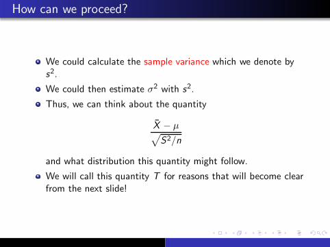
We could calculate the sample variance which we denote bys2.

How can we proceed?

We could calculate the sample variance which we denote bys2.

We could then estimate σ2 with s2.

How can we proceed?

We could calculate the sample variance which we denote bys2.

We could then estimate σ2 with s2.

Thus, we can think about the quantity

X̄ − µ√

S2/n

and what distribution this quantity might follow.

How can we proceed?

We could calculate the sample variance which we denote bys2.

We could then estimate σ2 with s2.

Thus, we can think about the quantity

X̄ − µ√

S2/n

and what distribution this quantity might follow.

We will call this quantity T for reasons that will become clearfrom the next slide!

Case 2: Unknown variance σ2

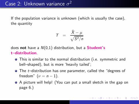
If the population variance is unknown (which is usually the case),the quantity

T =X̄ − µ√

S2/n

does not have a N(0,1) distribution, but a Student’s

t–distribution.

Case 2: Unknown variance σ2

If the population variance is unknown (which is usually the case),the quantity

T =X̄ − µ√

S2/n

does not have a N(0,1) distribution, but a Student’s

t–distribution.

This is similar to the normal distribution (i.e. symmetric andbell–shaped), but is more ‘heavily tailed’;

Case 2: Unknown variance σ2

If the population variance is unknown (which is usually the case),the quantity

T =X̄ − µ√

S2/n

does not have a N(0,1) distribution, but a Student’s

t–distribution.

This is similar to the normal distribution (i.e. symmetric andbell–shaped), but is more ‘heavily tailed’;

The t–distribution has one parameter, called the “degrees offreedom” (ν = n − 1).

Case 2: Unknown variance σ2

If the population variance is unknown (which is usually the case),the quantity

T =X̄ − µ√

S2/n

does not have a N(0,1) distribution, but a Student’s

t–distribution.

This is similar to the normal distribution (i.e. symmetric andbell–shaped), but is more ‘heavily tailed’;

The t–distribution has one parameter, called the “degrees offreedom” (ν = n − 1).

A picture will help! (You can put a small sketch in the gap onpage 6.)

comparison of Normal and T distributions

−10 −5 0 5 10

comparison of Normal and T distributions

−10 −5 0 5 10

Student’s t distribution – a brief history

Takes its name from William Sealy Gosset’s 1908 paper inBiometrika under the pseudonym ”Student”.

Gosset worked at the Guinness Brewery in Dublin, Ireland, andwas interested in the chemical properties of barley wheresample sizes might be small.

One version of the origin of the pseudonym is that Gosset’semployer forbade members of its staff from publishingscientific papers, so he had to hide his identity.

Another is that Guinness did not want their competitors toknow that they were using the t to test the quality of rawmaterial.

William Sealy Gosset 1876–1937

Back to our problem...

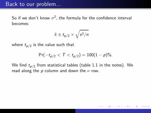
So if we don’t know σ2, the formula for the confidence intervalbecomes:

x̄ ± tp/2 ×

√

s2/n

Back to our problem...

So if we don’t know σ2, the formula for the confidence intervalbecomes:

x̄ ± tp/2 ×

√

s2/n

where tp/2 is the value such that

Pr(−tp/2 < T < tp/2) = 100(1 − p)%.

We find tp/2 from statistical tables (table 1.1 in the notes). Weread along the p column and down the ν row.

Back to our problem...

So if we don’t know σ2, the formula for the confidence intervalbecomes:

x̄ ± tp/2 ×

√

s2/n

where tp/2 is the value such that

Pr(−tp/2 < T < tp/2) = 100(1 − p)%.

We find tp/2 from statistical tables (table 1.1 in the notes). Weread along the p column and down the ν row.

For a 90% confidence interval, p = 10%.

For a 95% confidence interval, p = 5%.

For a 99% confidence interval, p = 1%.

The degrees of freedom, ν = n − 1.

Example (page 7)

A sample of size 15 is taken from a larger population; the samplemean is calculated as 12 and the sample variance as 25. What isthe 95% confidence interval for the population mean µ?

Example (page 7)

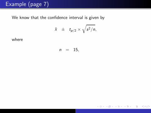
We know that the confidence interval is given by

x̄ ± tp/2 ×

√

s2/n,

where

Example (page 7)

We know that the confidence interval is given by

x̄ ± tp/2 ×

√

s2/n,

where

n = 15,

Example (page 7)

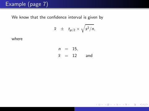
We know that the confidence interval is given by

x̄ ± tp/2 ×

√

s2/n,

where

n = 15,

x̄ = 12 and

Example (page 7)

We know that the confidence interval is given by

x̄ ± tp/2 ×

√

s2/n,

where

n = 15,

x̄ = 12 and

s2 = 25.

Also, to find t, we know that

ν = n − 1 = 15− 1 = 14 and

Example (page 7)

We know that the confidence interval is given by

x̄ ± tp/2 ×

√

s2/n,

where

n = 15,

x̄ = 12 and

s2 = 25.

Also, to find t, we know that

ν = n − 1 = 15− 1 = 14 and

p = 5%.

Example (page 7)

We can find our t value by looking in the p = 5% column and theν = 14 row, giving a value of 2.145.

Putting what we know into our expression, we get

12 ± t2.5% ×

√

25

15

Example (page 7)

We can find our t value by looking in the p = 5% column and theν = 14 row, giving a value of 2.145.

Putting what we know into our expression, we get

12 ± t2.5% ×

√

25

15

12 ± 2.145 ×

√

25

15i.e.

Example (page 7)

We can find our t value by looking in the p = 5% column and theν = 14 row, giving a value of 2.145.

Putting what we know into our expression, we get

12 ± t2.5% ×

√

25

15

12 ± 2.145 ×

√

25

15i.e.

12 ± 2.77.

Example (page 7)

We can find our t value by looking in the p = 5% column and theν = 14 row, giving a value of 2.145.

Putting what we know into our expression, we get

12 ± t2.5% ×

√

25

15

12 ± 2.145 ×

√

25

15i.e.

12 ± 2.77.

Hence, the confidence interval is (9.23, 14.77).

Write this down! (Bottom page 7)

It is claimed that µ = 9. Is this justified?

Write this down! (Bottom page 7)

It is claimed that µ = 9. Is this justified?

No! The claimed value of 9 does NOT lie within (9.23, 14.77).

Confidence intervals: a general approach

We now summarise the general procedure for calculating aconfidence interval for the population mean µ.

Confidence intervals: a general approach

We now summarise the general procedure for calculating aconfidence interval for the population mean µ.

Case 1: Known population variance σ2

(i) Calculate the sample mean x̄ from the data;

Confidence intervals: a general approach

We now summarise the general procedure for calculating aconfidence interval for the population mean µ.

Case 1: Known population variance σ2

(i) Calculate the sample mean x̄ from the data;

(ii) Calculate your interval! For example,

Confidence intervals: a general approach

We now summarise the general procedure for calculating aconfidence interval for the population mean µ.

Case 1: Known population variance σ2

(i) Calculate the sample mean x̄ from the data;

(ii) Calculate your interval! For example,for a 90% confidence interval, use the formula

x̄ ± 1.645×√

σ2/n;

Confidence intervals: a general approach

We now summarise the general procedure for calculating aconfidence interval for the population mean µ.

Case 1: Known population variance σ2

(i) Calculate the sample mean x̄ from the data;

(ii) Calculate your interval! For example,for a 90% confidence interval, use the formula

x̄ ± 1.645×√

σ2/n;

for a 95% confidence interval, use the formula

x̄ ± 1.96×√

σ2/n;

Confidence intervals: a general approach

We now summarise the general procedure for calculating aconfidence interval for the population mean µ.

Case 1: Known population variance σ2

(i) Calculate the sample mean x̄ from the data;

(ii) Calculate your interval! For example,for a 90% confidence interval, use the formula

x̄ ± 1.645×√

σ2/n;

for a 95% confidence interval, use the formula

x̄ ± 1.96×√

σ2/n;

for a 99% confidence interval, use the formula

x̄ ± 2.576×√

σ2/n.

Confidence intervals: a general approach

Case 2: Unknown population variance σ2

Confidence intervals: a general approach

Case 2: Unknown population variance σ2

(i) Calculate the sample mean x̄ and the sample variance s2 fromthe data;

Confidence intervals: a general approach

Case 2: Unknown population variance σ2

(i) Calculate the sample mean x̄ and the sample variance s2 fromthe data;

(ii) For a 100(1 − p)% confidence interval, look up the value of tunder column p, row ν of table 1.1, remembering thatν = n − 1.Note that, for a 90% confidence interval, p = 10%, for a 95%confidence interval, p = 5% and for a 99% confidenceinterval, p = 1%;

Confidence intervals: a general approach

Case 2: Unknown population variance σ2

(i) Calculate the sample mean x̄ and the sample variance s2 fromthe data;

(ii) For a 100(1 − p)% confidence interval, look up the value of tunder column p, row ν of table 1.1, remembering thatν = n − 1.Note that, for a 90% confidence interval, p = 10%, for a 95%confidence interval, p = 5% and for a 99% confidenceinterval, p = 1%;

(iii) Calculate your interval, using

x̄ ± tp/2 ×

√

s2/n.

Application of Confidence Intervals

You might be asking: “why do we bother calculating confidenceintervals?”.

Application of Confidence Intervals

You might be asking: “why do we bother calculating confidenceintervals?”.

By calculating a confidence interval for the population mean,it allows us to see how confident we are of the point estimatewe have calculated. The wider the range, the less precise wecan be about the population value.

Application of Confidence Intervals

You might be asking: “why do we bother calculating confidenceintervals?”.

By calculating a confidence interval for the population mean,it allows us to see how confident we are of the point estimatewe have calculated. The wider the range, the less precise wecan be about the population value.

If we have a known (or target) value for a population and thisdoes not fall within the confidence interval of our sample, thiscould suggest that there is something different about thissample.

Application of Confidence Intervals

You might be asking: “why do we bother calculating confidenceintervals?”.

By calculating a confidence interval for the population mean,it allows us to see how confident we are of the point estimatewe have calculated. The wider the range, the less precise wecan be about the population value.

If we have a known (or target) value for a population and thisdoes not fall within the confidence interval of our sample, thiscould suggest that there is something different about thissample.

It allows us to start looking at differences between groups. Ifthe confidence intervals for two samples do not overlap, thiscould suggest that they are from separate populations.

Example (page 8)

A credit card company wants to determine the mean income of itscard holders. It also wants to find out if there are any differencesin mean income between males and females.

Example (page 8)

A random sample of 225 male card holders and 190 female cardholders was drawn, and the following results obtained:

Mean Standard deviation

Males £16 450 £3675Females £13 220 £3050

Calculate 95% confidence intervals for the mean income for malesand females. Is there any evidence to suggest that, on average,males’ and females’ incomes differ? If so, describe this difference.

Example (page 8)

95% confidence interval for male income

The true population variance, σ2, is unknown, and so we have case2 and need to use the t distribution. Thus,

Example (page 8)

95% confidence interval for male income

The true population variance, σ2, is unknown, and so we have case2 and need to use the t distribution. Thus,

x̄ ± tp/2 ×

√

s2/n.

Example (page 8)

95% confidence interval for male income

The true population variance, σ2, is unknown, and so we have case2 and need to use the t distribution. Thus,

x̄ ± tp/2 ×

√

s2/n.

Here,

x̄ = 16450,

s2 = 36752 = 13505625 and

n = 225.

Example (page 8)

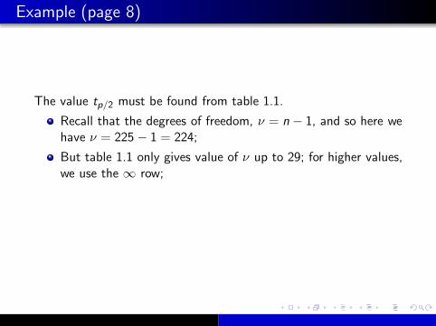
The value tp/2 must be found from table 1.1.

Example (page 8)

The value tp/2 must be found from table 1.1.

Recall that the degrees of freedom, ν = n − 1, and so here wehave ν = 225 − 1 = 224;

Example (page 8)

The value tp/2 must be found from table 1.1.

Recall that the degrees of freedom, ν = n − 1, and so here wehave ν = 225 − 1 = 224;

But table 1.1 only gives value of ν up to 29; for higher values,we use the ∞ row;

Example (page 8)

The value tp/2 must be found from table 1.1.

Recall that the degrees of freedom, ν = n − 1, and so here wehave ν = 225 − 1 = 224;

But table 1.1 only gives value of ν up to 29; for higher values,we use the ∞ row;

Since we require a 95% confidence interval, we read down the5% column, giving a t value of 1.96.

Example (page 8)

Thus, the 95% confidence interval for µ is found as

Example (page 8)

Thus, the 95% confidence interval for µ is found as

16450 ± 1.96 ×√

13505625/225, i.e.

Example (page 8)

Thus, the 95% confidence interval for µ is found as

16450 ± 1.96 ×√

13505625/225, i.e.

16450 ± 480.2.

Example (page 8)

Thus, the 95% confidence interval for µ is found as

16450 ± 1.96 ×√

13505625/225, i.e.

16450 ± 480.2.

So, the 95% confidence interval is (£15969.80,£16930.20).

Example (page 9)

95% confidence interval for female income

Again, the true population variance, σ2, is unknown, and so wehave case 2. Thus,

Example (page 9)

95% confidence interval for female income

Again, the true population variance, σ2, is unknown, and so wehave case 2. Thus,

x̄ ± tp/2 ×

√

s2/n.

Example (page 9)

95% confidence interval for female income

Again, the true population variance, σ2, is unknown, and so wehave case 2. Thus,

x̄ ± tp/2 ×

√

s2/n.

Now,

x̄ = 13220,

s2 = 30502

= 9302500, and

n = 190.

Example (page 9)

Again, since the sample size is large, we use the ∞ row of table1.1 to obtain the value of tp/2, giving:

Example (page 9)

Again, since the sample size is large, we use the ∞ row of table1.1 to obtain the value of tp/2, giving:

13220 ± 1.96×√

9302500/190, i.e.

Example (page 9)

Again, since the sample size is large, we use the ∞ row of table1.1 to obtain the value of tp/2, giving:

13220 ± 1.96×√

9302500/190, i.e.

13220 ± 1.96× 221.27, i.e.

Example (page 9)

Again, since the sample size is large, we use the ∞ row of table1.1 to obtain the value of tp/2, giving:

13220 ± 1.96×√

9302500/190, i.e.

13220 ± 1.96× 221.27, i.e.

13220 ± 433.69.

Example (page 9)

Again, since the sample size is large, we use the ∞ row of table1.1 to obtain the value of tp/2, giving:

13220 ± 1.96×√

9302500/190, i.e.

13220 ± 1.96× 221.27, i.e.

13220 ± 433.69.

So, the 95% confidence interval is (£12786.31,£13653.69).

Example (page 9)

Since the 95% confidence intervals for males and females do not

overlap, there is evidence to suggest that males’ and females’incomes, on average, are different.

Further, it appears that male card holders earn more than women.

But note that the dataset is rather old...