lecture 2: linear and quadratic classifiers
TRANSCRIPT
Introduction to Pattern AnalysisRicardo Gutierrez-OsunaTexas A&M University
1
LECTURE 2: Linear and quadratic classifiers
g Part 1: Bayesian Decision Theoryn The Likelihood Ratio Testn Maximum A Posteriori and Maximum Likelihoodn Discriminant functions
g Part 2: Quadratic classifiersn Bayes classifiers for normally distributed classesn Euclidean and Mahalanobis distance classifiersn Numerical example
g Part 3: Linear classifiersn Gradient descentn The perceptron rulen The pseudo-inverse solutionn Least mean squares
Introduction to Pattern AnalysisRicardo Gutierrez-OsunaTexas A&M University
2
Part 1: Bayesian Decision Theory
Introduction to Pattern AnalysisRicardo Gutierrez-OsunaTexas A&M University
3
The Likelihood Ratio Test (1)g Assume we are to classify an object based on the
evidence provided by a measurement (or feature vector) x
g Would you agree that a reasonable decision rule would be the following?
n "Choose the class that is most ‘probable’ given the observed feature vector x”
n More formally: Evaluate the posterior probability of each class P(ωi|x) and choose the class with largest P(ωi|x)
Introduction to Pattern AnalysisRicardo Gutierrez-OsunaTexas A&M University
4
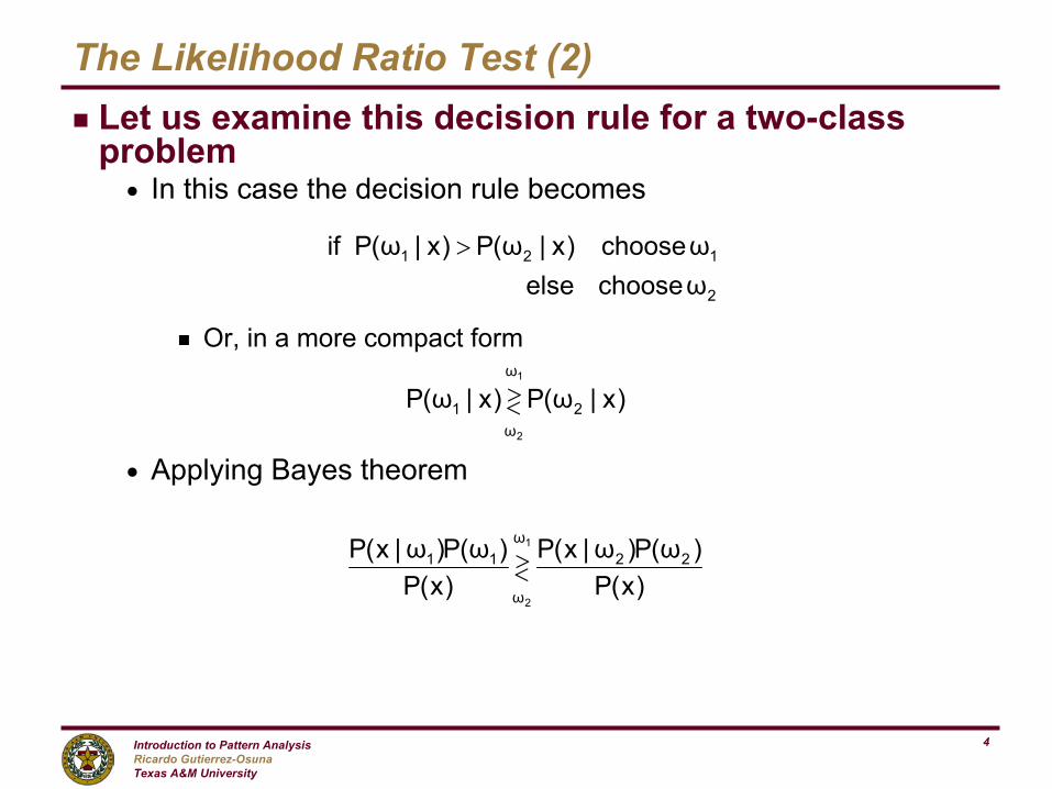
The Likelihood Ratio Test (2)g Let us examine this decision rule for a two-class
problemn In this case the decision rule becomes
g Or, in a more compact form
n Applying Bayes theorem
2
121
ωchooseelseωchoose)x|ω(P)x|ω(Pif >
)x|ω(P)x|ω(P 2
ω
ω1
1
2
<>
)x(P)ω(P)ω|x(P
)x(P)ω(P)ω|x(P 22ω
ω
111
2
<>
Introduction to Pattern AnalysisRicardo Gutierrez-OsunaTexas A&M University
5
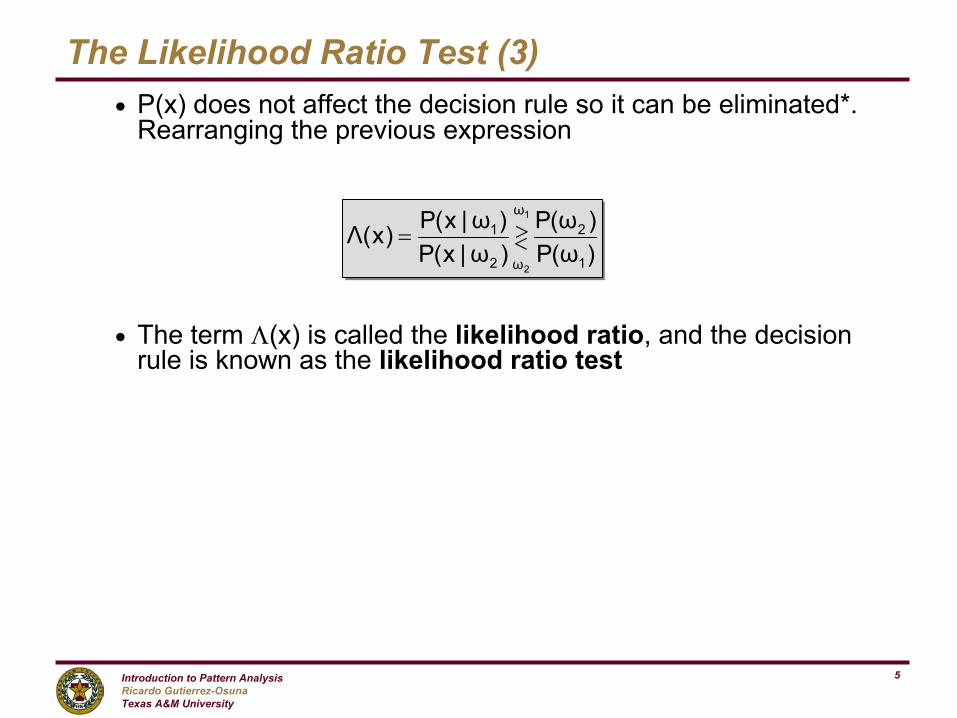
The Likelihood Ratio Test (3)n P(x) does not affect the decision rule so it can be eliminated*.
Rearranging the previous expression
n The term Λ(x) is called the likelihood ratio, and the decision rule is known as the likelihood ratio test
)ω(P)ω(P
)ω|x(P)ω|x(P)x(Λ
1
2ω
ω2
11
2
<>=
Introduction to Pattern AnalysisRicardo Gutierrez-OsunaTexas A&M University
6
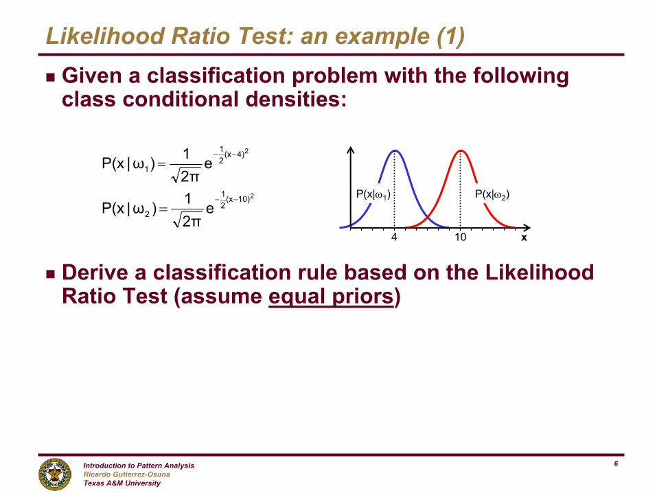
Likelihood Ratio Test: an example (1)g Given a classification problem with the following
class conditional densities:
g Derive a classification rule based on the Likelihood Ratio Test (assume equal priors)
2
2
10)(x21
2
4)(x21
1
e2π1)ω|P(x
e2π1)ω|P(x
−−
−−
=
=
x
P(x|ω1) P(x|ω2)
4 10
Introduction to Pattern AnalysisRicardo Gutierrez-OsunaTexas A&M University
7
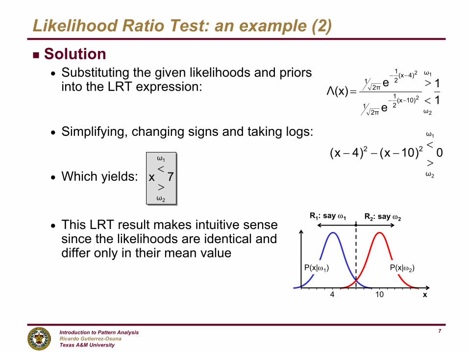
Likelihood Ratio Test: an example (2)g Solution
n Substituting the given likelihoods and priors into the LRT expression:
n Simplifying, changing signs and taking logs:
n Which yields:
n This LRT result makes intuitive sense since the likelihoods are identical and differ only in their mean value
11
e
eΛ(x)
1
2
2
2 ω
ω10)(x
21
2π1
4)(x21
2π1
<>
=−−
−−
0)10x()4x(1
2
ω
ω
22
><
−−−
7x1
2
ω
ω><
R1: say ω1
x
R2: say ω2
P(x|ω1) P(x|ω2)
4 10
Introduction to Pattern AnalysisRicardo Gutierrez-OsunaTexas A&M University
8
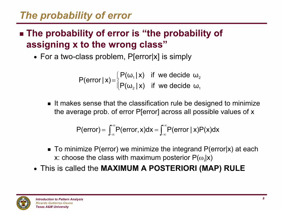
The probability of error
g The probability of error is “the probability of assigning x to the wrong class”n For a two-class problem, P[error|x] is simply
g It makes sense that the classification rule be designed to minimize the average prob. of error P[error] across all possible values of x
g To minimize P(error) we minimize the integrand P(error|x) at each x: choose the class with maximum posterior P(ωi|x)
n This is called the MAXIMUM A POSTERIORI (MAP) RULE
=12
21
ωdecideweifx)|P(ωωdecideweifx)|P(ω
x)|P(error
∫∫+∞
∞−
+∞
∞−== x)P(x)dx|P(errorx)dxP(error,P(error)
Introduction to Pattern AnalysisRicardo Gutierrez-OsunaTexas A&M University
9
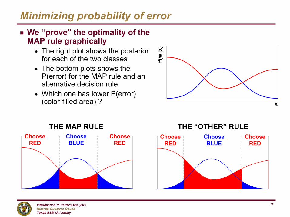
Minimizing probability of errorg We “prove” the optimality of the
MAP rule graphicallyn The right plot shows the posterior
for each of the two classesn The bottom plots shows the
P(error) for the MAP rule and an alternative decision rule
n Which one has lower P(error) (color-filled area) ? x
P(w
i|x)
ChooseRED
ChooseBLUE
ChooseRED
THE MAP RULEChoose
REDChooseBLUE
ChooseRED
THE “OTHER” RULE
Introduction to Pattern AnalysisRicardo Gutierrez-OsunaTexas A&M University
10
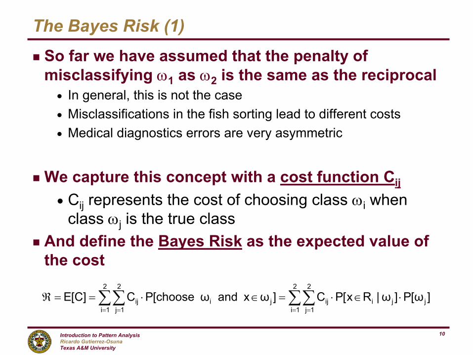
The Bayes Risk (1)
g So far we have assumed that the penalty of misclassifying ω1 as ω2 is the same as the reciprocaln In general, this is not the casen Misclassifications in the fish sorting lead to different costs n Medical diagnostics errors are very asymmetric
g We capture this concept with a cost function Cij
n Cij represents the cost of choosing class ωi when class ωj is the true class
g And define the Bayes Risk as the expected value of the cost
∑∑∑∑= == =
⋅∈⋅=∈⋅==ℜ2
1i
2
1jjjiij
2
1i
2
1jjiij ]ω[P]ω|Rx[PC]ωxandωchoose[PC]C[E
Introduction to Pattern AnalysisRicardo Gutierrez-OsunaTexas A&M University
11
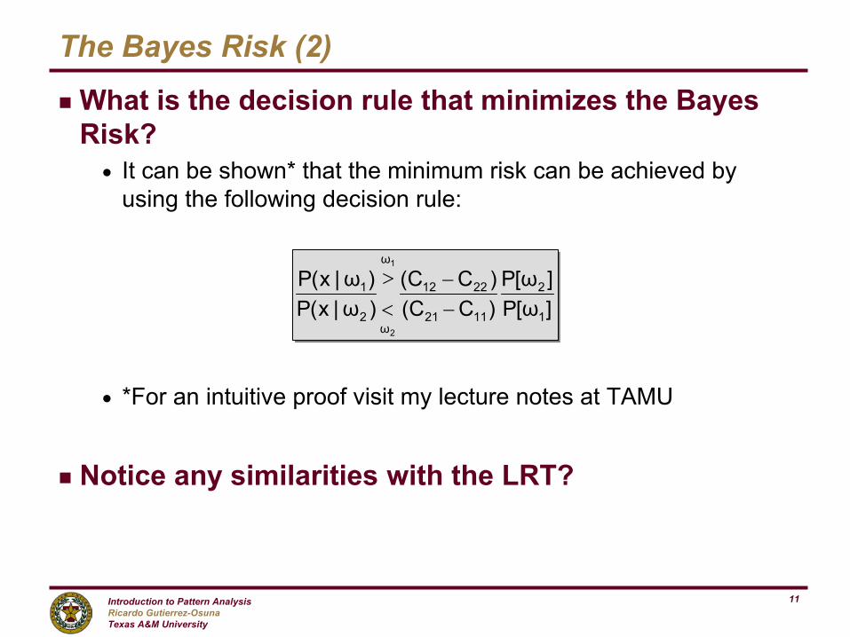
The Bayes Risk (2)
g What is the decision rule that minimizes the Bayes Risk?n It can be shown* that the minimum risk can be achieved by
using the following decision rule:
n *For an intuitive proof visit my lecture notes at TAMU
g Notice any similarities with the LRT?
]ω[P]ω[P
)CC()CC(
)ω|x(P)ω|x(P
1
2
1121
2212
ω
ω2
1
1
2
−−
<>
Introduction to Pattern AnalysisRicardo Gutierrez-OsunaTexas A&M University
12
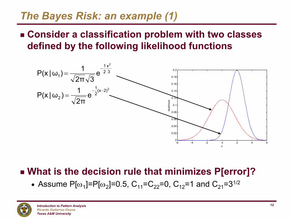
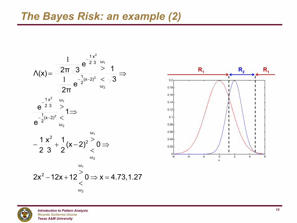
The Bayes Risk: an example (1)
g Consider a classification problem with two classes defined by the following likelihood functions
g What is the decision rule that minimizes P[error]?n Assume P[ω1]=P[ω2]=0.5, C11=C22=0, C12=1 and C21=31/2
2
2
2)(x21
2
3x
21
1
e2π1)ω|P(x
e32π
1)ω|P(x
−−
−
=
=
-6 -4 -2 0 2 4 60
0.02
0.04
0.06
0.08
0.1
0.12
0.14
0.16
0.18
0.2
x
likel
ihoo
d
Introduction to Pattern AnalysisRicardo Gutierrez-OsunaTexas A&M University
13
The Bayes Risk: an example (2)
1.274.73,x01212x2x
02)(x21
3x
21
1e
e
31
e2π
e32πΛ(x)
1
2
1
2
1
2
2
2
1
2
2
2
ω
ω
2
ω
ω
22
ω
ω2)(x
21
3x
21
ω
ω2)(x
21
3x
21
=⇒<>
+−
⇒<>
−+−
⇒<>
⇒<>
=
−−
−
−−
−
1
1
-6 -4 -2 0 2 4 60
0.02
0.04
0.06
0.08
0.1
0.12
0.14
0.16
0.18
0.2
x
R1R2R1
Introduction to Pattern AnalysisRicardo Gutierrez-OsunaTexas A&M University
14
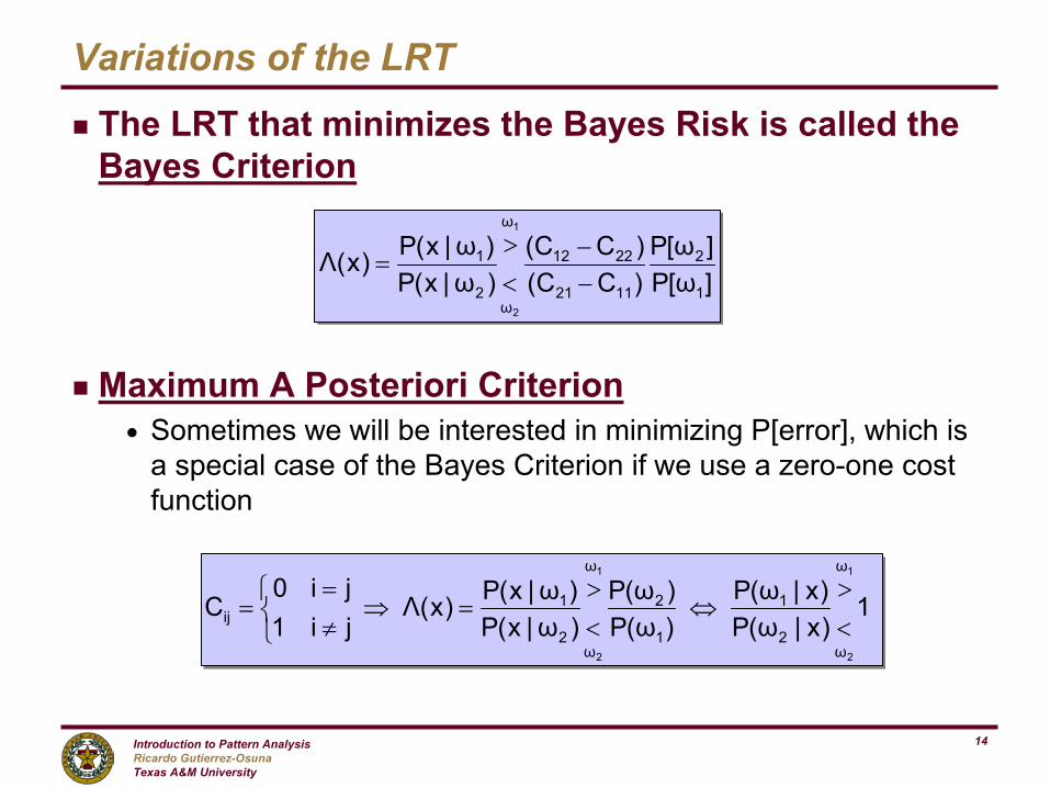
g The LRT that minimizes the Bayes Risk is called the Bayes Criterion
g Maximum A Posteriori Criterionn Sometimes we will be interested in minimizing P[error], which is
a special case of the Bayes Criterion if we use a zero-one cost function
Variations of the LRT
]ω[P]ω[P
)CC()CC(
)ω|x(P)ω|x(P)x(Λ
1
2
1121
2212
ω
ω2
1
1
2
−−
<>
=
1)x|ω(P)x|ω(P
)ω(P)ω(P
)ω|x(P)ω|x(P)x(Λ
ji1ji0
C1
2
1
2
ω
ω2
1
1
2
ω
ω2
1ij <
>⇔
<>
=⇒
≠=
=
Introduction to Pattern AnalysisRicardo Gutierrez-OsunaTexas A&M University
15
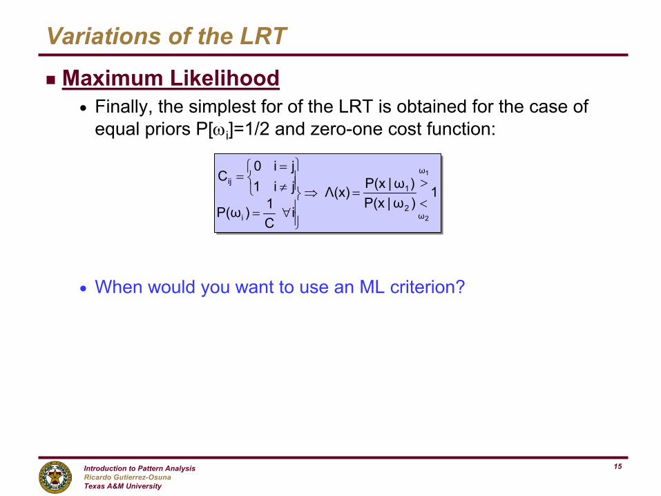
g Maximum Likelihoodn Finally, the simplest for of the LRT is obtained for the case of
equal priors P[ωi]=1/2 and zero-one cost function:
n When would you want to use an ML criterion?
Variations of the LRT
1)ω|P(x)ω|P(xΛ(x)
iC1)P(ω
ji1ji0
C 1
2
ω
ω2
1
i
ij
<>
=⇒
∀=
≠=
=
Introduction to Pattern AnalysisRicardo Gutierrez-OsunaTexas A&M University
16
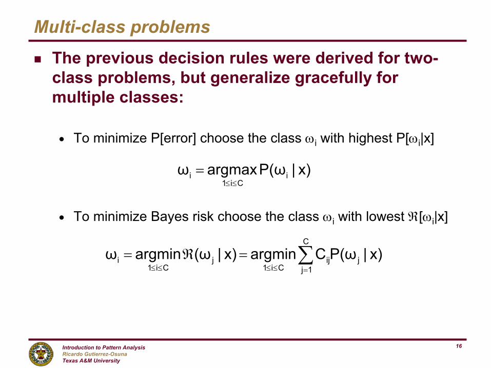
Multi-class problems
g The previous decision rules were derived for two-class problems, but generalize gracefully for multiple classes:
n To minimize P[error] choose the class ωi with highest P[ωi|x]
n To minimize Bayes risk choose the class ωi with lowest ℜ[ωi|x]
∑=≤≤≤≤
=ℜ=C
1jjij
Ci1j
Ci1i x)|P(ωCargminx)|(ωargminω
x)|P(ωargmaxω iCi1
i≤≤
=
Introduction to Pattern AnalysisRicardo Gutierrez-OsunaTexas A&M University
17
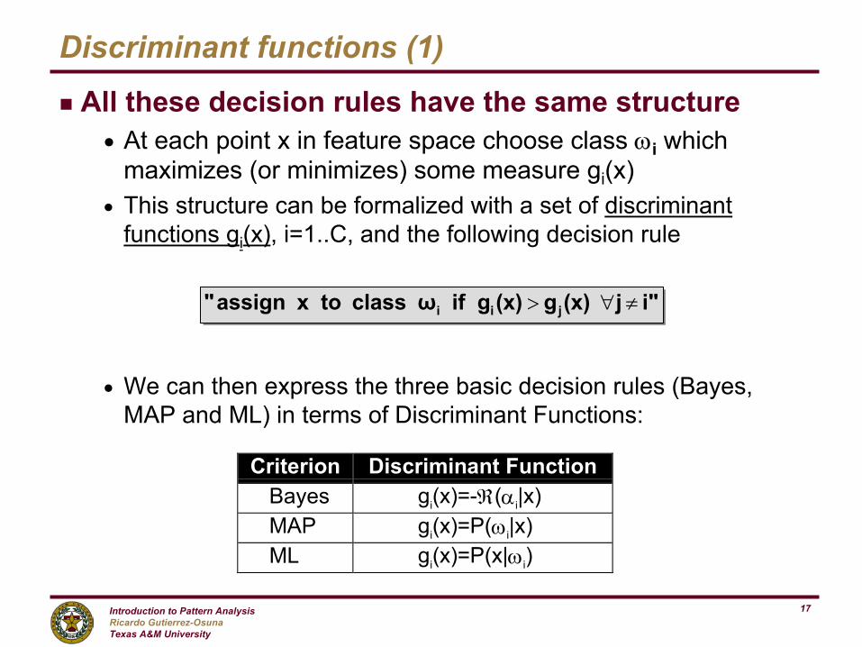
Discriminant functions (1)
g All these decision rules have the same structuren At each point x in feature space choose class ωi which
maximizes (or minimizes) some measure gi(x)n This structure can be formalized with a set of discriminant
functions gi(x), i=1..C, and the following decision rule
n We can then express the three basic decision rules (Bayes, MAP and ML) in terms of Discriminant Functions:
i"j(x)g(x)gifωclasstoxassign" jii ≠∀>
Criterion Discriminant FunctionBayes gi(x)=-ℜ(αi|x)MAP gi(x)=P(ωi|x)ML gi(x)=P(x|ωi)
Introduction to Pattern AnalysisRicardo Gutierrez-OsunaTexas A&M University
18
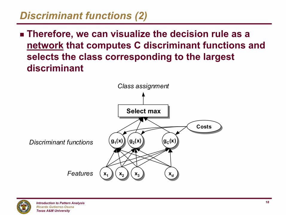
Discriminant functions (2)
g Therefore, we can visualize the decision rule as a network that computes C discriminant functions and selects the class corresponding to the largest discriminant
x2x2 x3
x3 xdxd
g1(x)g1(x)
x1x1
g2(x)g2(x) gC(x)gC(x)
Select maxSelect max
CostsCosts
Class assignment
Discriminant functions
Features
Introduction to Pattern AnalysisRicardo Gutierrez-OsunaTexas A&M University
19
Recapping…
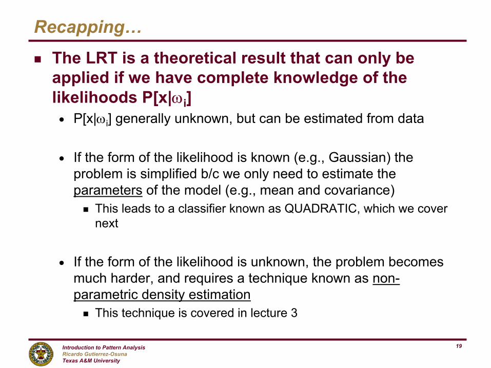
g The LRT is a theoretical result that can only be applied if we have complete knowledge of the likelihoods P[x|ωi]n P[x|ωi] generally unknown, but can be estimated from data
n If the form of the likelihood is known (e.g., Gaussian) the problem is simplified b/c we only need to estimate the parameters of the model (e.g., mean and covariance)g This leads to a classifier known as QUADRATIC, which we cover
next
n If the form of the likelihood is unknown, the problem becomes much harder, and requires a technique known as non-parametric density estimationg This technique is covered in lecture 3
Introduction to Pattern AnalysisRicardo Gutierrez-OsunaTexas A&M University
20
Part 2: Quadratic classifiers
Introduction to Pattern AnalysisRicardo Gutierrez-OsunaTexas A&M University
21
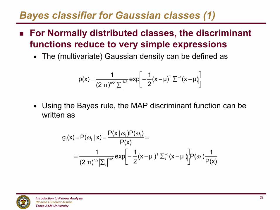
Bayes classifier for Gaussian classes (1)
g For Normally distributed classes, the discriminant functions reduce to very simple expressionsn The (multivariate) Gaussian density can be defined as
n Using the Bayes rule, the MAP discriminant function can be written as
−∑−−
∑= − µ)(xµ)(x
21exp
π)(21p(x) 1T
1/2n/2
P(x)1)P()µ(x)µ(x
21exp
π)(21
P(x)))P(|P(xx)|P((x)g
iiT
i1/2n/2
iiii
ω
ωωω
−∑−−
∑=
===
−1i
i
Introduction to Pattern AnalysisRicardo Gutierrez-OsunaTexas A&M University
22
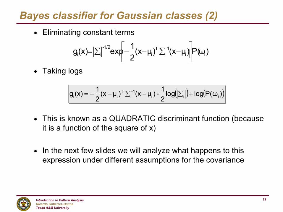
Bayes classifier for Gaussian classes (2)n Eliminating constant terms
n Taking logs
n This is known as a QUADRATIC discriminant function (because it is a function of the square of x)
n In the next few slides we will analyze what happens to this expression under different assumptions for the covariance
( ) ( ))ωP(loglog21-)µ(x)µ(x
21(x)g iii
1i
Tii +∑−∑−−= −
)ωP()µ(x)µ(x21exp(x)g ii
1i
Ti
1/2-ii
−∑−−∑= −
Introduction to Pattern AnalysisRicardo Gutierrez-OsunaTexas A&M University
23
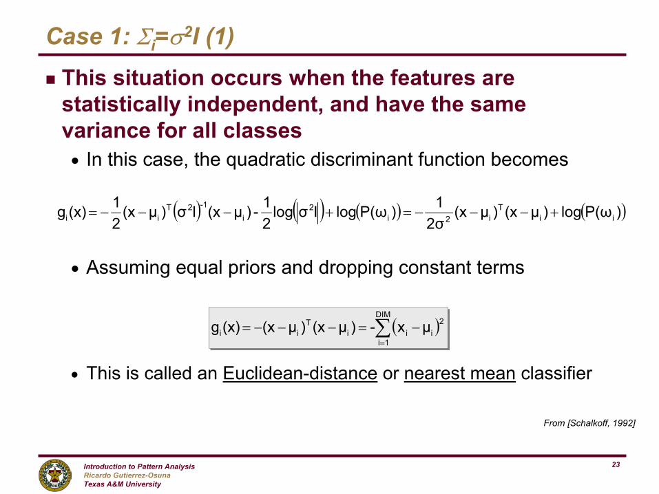
Case 1: Σi=σ2I (1)g This situation occurs when the features are
statistically independent, and have the same variance for all classesn In this case, the quadratic discriminant function becomes
n Assuming equal priors and dropping constant terms
n This is called an Euclidean-distance or nearest mean classifier
( ) ( ) ( ) ( ))P(ωlog)µ(x)µ(x2σ
1)P(ωlogIσlog21-)µ(xIσ)µ(x
21(x)g ii
Ti2i
2i
-12Tii +−−−=+−−−=
( )∑=
−=−−−=DIM
1i
2iii
Tii µx-)µ(x)µ(x(x)g
From [Schalkoff, 1992]
Introduction to Pattern AnalysisRicardo Gutierrez-OsunaTexas A&M University
24
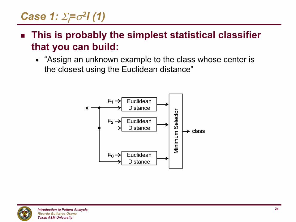
Case 1: Σi=σ2I (1)g This is probably the simplest statistical classifier
that you can build:n “Assign an unknown example to the class whose center is
the closest using the Euclidean distance”
µ1
Min
imum
Sel
ecto
r
µ2
µC
class
xEuclidean Distance
Euclidean Distance
Euclidean Distance
µ1
Min
imum
Sel
ecto
r
µ2
µC
class
xEuclidean Distance
Euclidean Distance
Euclidean Distance
Introduction to Pattern AnalysisRicardo Gutierrez-OsunaTexas A&M University
25
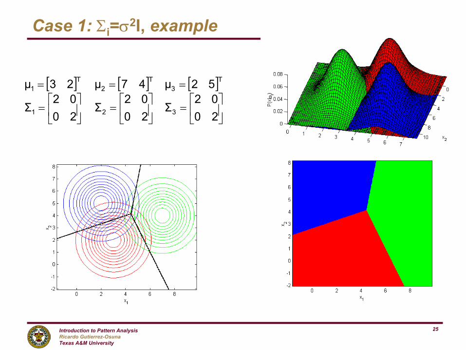
Case 1: Σi=σ2I, example
[ ] [ ] [ ]
=
=
=
===
2002
Σ2002
Σ2002
Σ
52µ47µ23µ
321
T3
T2
T1
Introduction to Pattern AnalysisRicardo Gutierrez-OsunaTexas A&M University
26
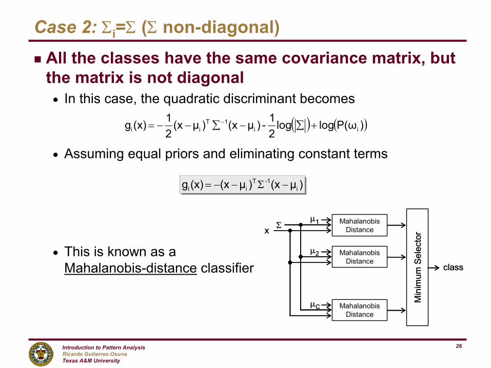
Case 2: Σi=Σ (Σ non-diagonal)g All the classes have the same covariance matrix, but
the matrix is not diagonaln In this case, the quadratic discriminant becomes
n Assuming equal priors and eliminating constant terms
n This is known as a Mahalanobis-distance classifier
( ) ( ))P(ωloglog21-)µ(x)µ(x
21(x)g ii
1Tii +∑−∑−−= −
)µ(x)µ(x(x)g i-1T
ii −Σ−−=
µ1
Min
imum
Sel
ecto
r
µ2
µC
class
xMahalanobis
Distance
Mahalanobis Distance
Mahalanobis Distance
Σµ1
Min
imum
Sel
ecto
r
µ2
µC
class
xMahalanobis
Distance
Mahalanobis Distance
Mahalanobis Distance
Σ
Introduction to Pattern AnalysisRicardo Gutierrez-OsunaTexas A&M University
27
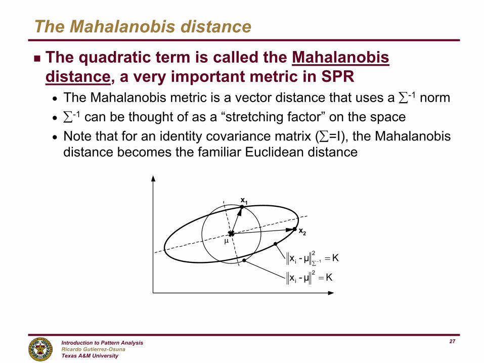
The Mahalanobis distance
g The quadratic term is called the Mahalanobis distance, a very important metric in SPRn The Mahalanobis metric is a vector distance that uses a ∑-1 normn ∑-1 can be thought of as a “stretching factor” on the spacen Note that for an identity covariance matrix (∑=I), the Mahalanobis
distance becomes the familiar Euclidean distance
µx2
x1
Κ µ-x 2i =
K µ-x 2i 1 =−∑
Introduction to Pattern AnalysisRicardo Gutierrez-OsunaTexas A&M University
28
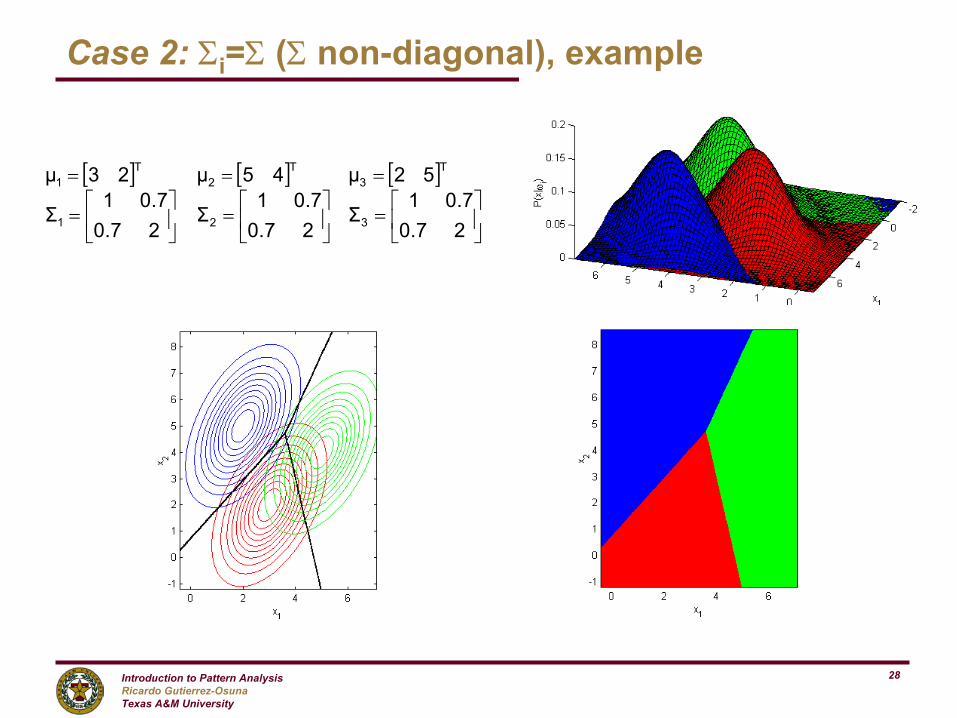
[ ] [ ] [ ]
=
=
=
===
27.07.01
Σ27.07.01
Σ27.07.01
Σ
52µ45µ23µ
321
T3
T2
T1
Case 2: Σi=Σ (Σ non-diagonal), example
Introduction to Pattern AnalysisRicardo Gutierrez-OsunaTexas A&M University
29
[ ] [ ] [ ]
=
−
−=
−
−=
===
35.05.05.0
Σ7111
Σ2111
Σ
52µ45µ23µ
321
T3
T2
T1
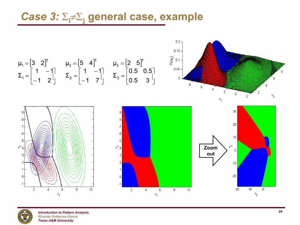
Case 3: Σi≠Σj general case, example
Zoomout
Introduction to Pattern AnalysisRicardo Gutierrez-OsunaTexas A&M University
30
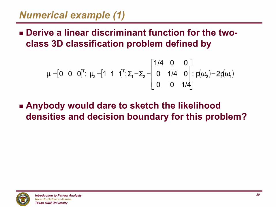
Numerical example (1)
g Derive a linear discriminant function for the two-class 3D classification problem defined by
g Anybody would dare to sketch the likelihood densities and decision boundary for this problem?
[ ] [ ] ( ) ( )1221T
2T
1 ω2pωp;1/40001/40001/4
ΣΣ ;111µ;000µ =
====
Introduction to Pattern AnalysisRicardo Gutierrez-OsunaTexas A&M University
31
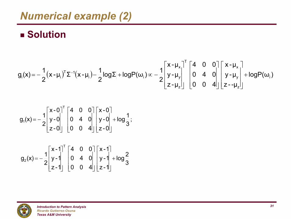
Numerical example (2)
g Solution
( ) ( ) )logP(ω-µ-zµ-yµ-x
400040004
µ-zµ-yµ-x
21)logP(ωΣlog
21µ-xΣµ-x
21(x)g i
z
y
xT
z
y
x
ii1T
ii +
−∝+−−= −
32log
1-z1-y1-x
400040004
1-z1-y1-x
21(x)g
31log
0-z0-y0-x
400040004
0-z0-y0-x
21(x)g
T
2
T
1
+
−=
+
−= ;
Introduction to Pattern AnalysisRicardo Gutierrez-OsunaTexas A&M University
32
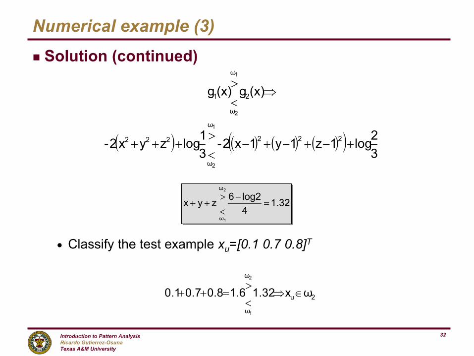
Numerical example (3)
g Solution (continued)
n Classify the test example xu=[0.1 0.7 0.8]T
( ) ( ) ( ) ( )( )32log1z1y1x2-
31logzyx2-
(x)g(x)g
222
ω
ω
222
2
ω
ω
1
2
1
2
1
+−+−+−<>
+++
⇒<>
1.324log26 zyx
1
2
ω
ω
=−
<>
++
2u
ω
ω
ωx1.321.6 0.80.70.11
2
∈⇒<>
=++
Introduction to Pattern AnalysisRicardo Gutierrez-OsunaTexas A&M University
33
Conclusions
g The Euclidean distance classifier is Bayes-optimal* ifn Gaussian classes and equal covariance matrices proportional to
the identity matrix and equal priors
g The Mahalanobis dist. classifier is Bayes-optimal ifn Gaussian classes and equal covariance matrices and equal
priors
*Bayes optimal means that the classifier yields the minimum P[error], which is the best ANY classifier can achieve
Introduction to Pattern AnalysisRicardo Gutierrez-OsunaTexas A&M University
34
Part 3: Linear classifiers
Introduction to Pattern AnalysisRicardo Gutierrez-OsunaTexas A&M University
35
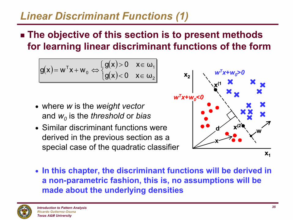
Linear Discriminant Functions (1)
g The objective of this section is to present methods for learning linear discriminant functions of the form
n where w is the weight vectorand w0 is the threshold or bias
n Similar discriminant functions were derived in the previous section as a special case of the quadratic classifier
n In this chapter, the discriminant functions will be derived in a non-parametric fashion, this is, no assumptions will be made about the underlying densities
x1
x2
wx
wTx+w0>0
wTx+w0<0
x(1
x(2d
x1
x2
wx
wTx+w0>0
wTx+w0<0
x(1
x(2d
( ) ( )( )
∈<∈>
⇔+=2
10
T
ωx0xgωx0xg
wxwxg
Introduction to Pattern AnalysisRicardo Gutierrez-OsunaTexas A&M University
36
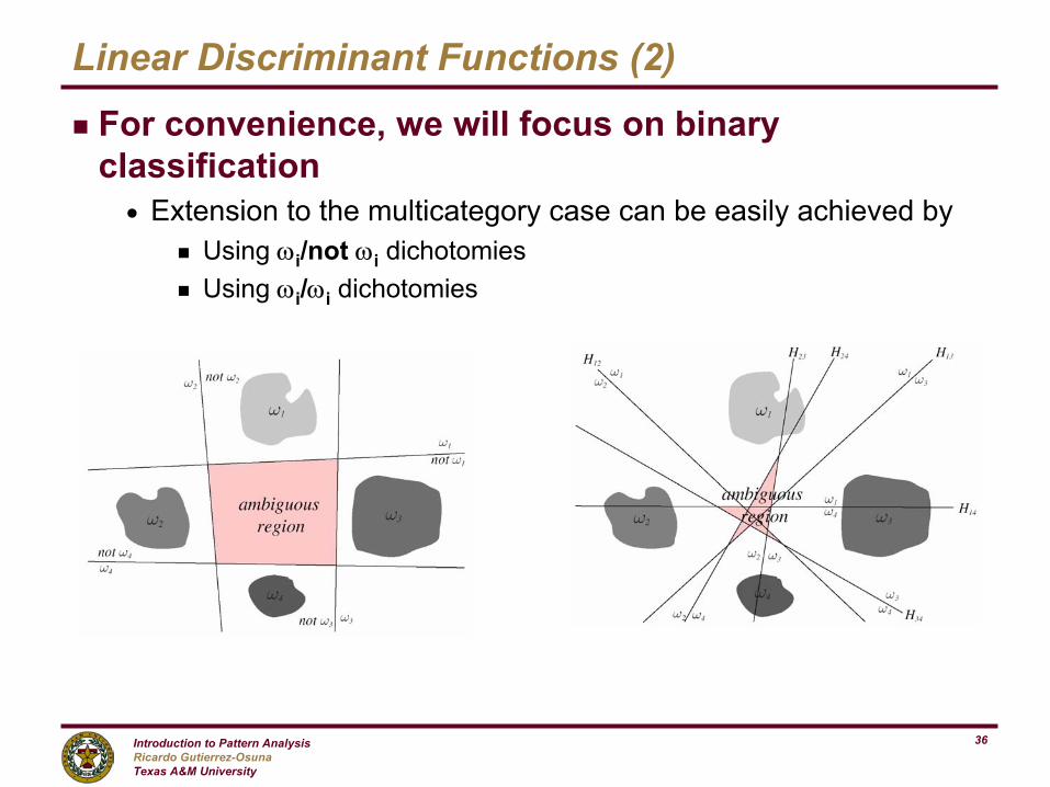
Linear Discriminant Functions (2)
g For convenience, we will focus on binary classificationn Extension to the multicategory case can be easily achieved by
g Using ωi/not ωi dichotomiesg Using ωi/ωi dichotomies
Introduction to Pattern AnalysisRicardo Gutierrez-OsunaTexas A&M University
37
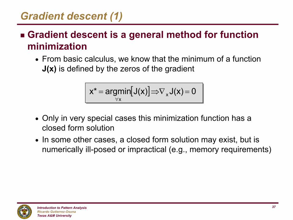
Gradient descent (1)
g Gradient descent is a general method for function minimization n From basic calculus, we know that the minimum of a function
J(x) is defined by the zeros of the gradient
n Only in very special cases this minimization function has a closed form solution
n In some other cases, a closed form solution may exist, but is numerically ill-posed or impractical (e.g., memory requirements)
[ ] 0J(x)J(x)argminx* xx
=⇒∇=∀
Introduction to Pattern AnalysisRicardo Gutierrez-OsunaTexas A&M University
38
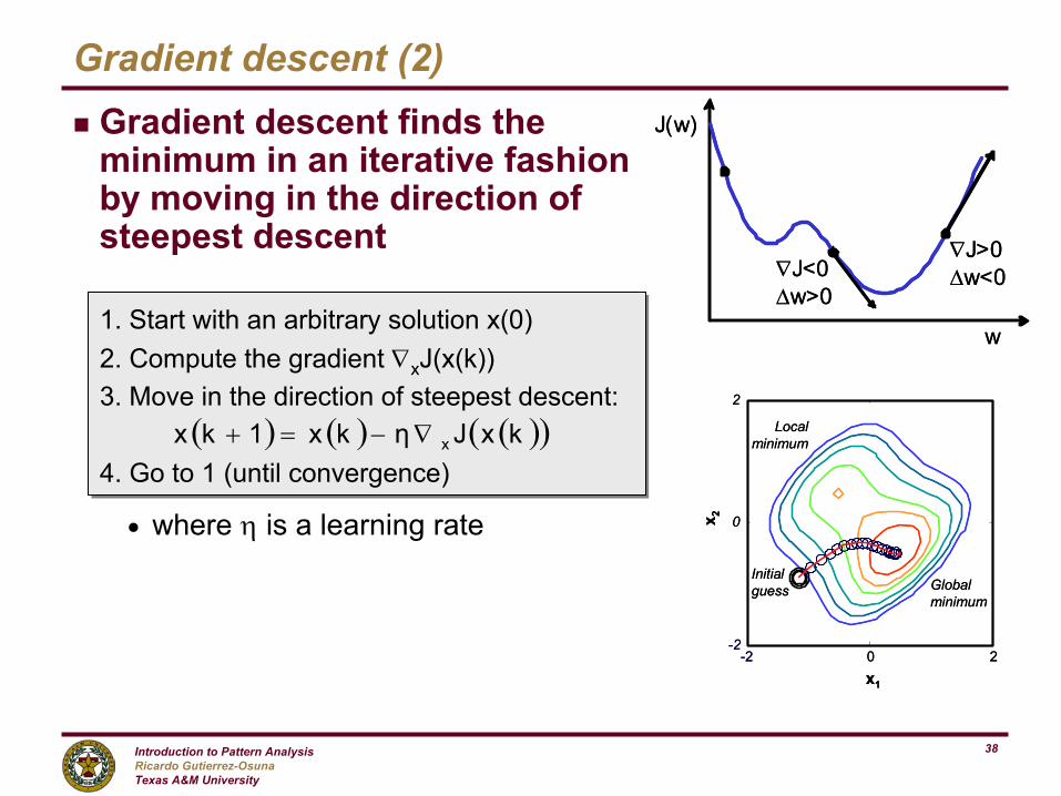
Gradient descent (2)g Gradient descent finds the
minimum in an iterative fashion by moving in the direction of steepest descent
n where η is a learning rate
1. Start with an arbitrary solution x(0)2. Compute the gradient ∇xJ(x(k))3. Move in the direction of steepest descent:
4. Go to 1 (until convergence)
1. Start with an arbitrary solution x(0)2. Compute the gradient ∇xJ(x(k))3. Move in the direction of steepest descent:
4. Go to 1 (until convergence)( ) ( ) ( )( )kxJηkx1kx x∇−=+
-2 0 2-2
0
2
x1
x 2
Initialguess Global
minimum
Localminimum
-2 0 2-2
0
2
x1
x 2
Initialguess Global
minimum
Localminimum
J(w)
w
∇J<0∆w>0
∇J>0∆w<0
J(w)
w
∇J<0∆w>0
∇J>0∆w<0
Introduction to Pattern AnalysisRicardo Gutierrez-OsunaTexas A&M University
39
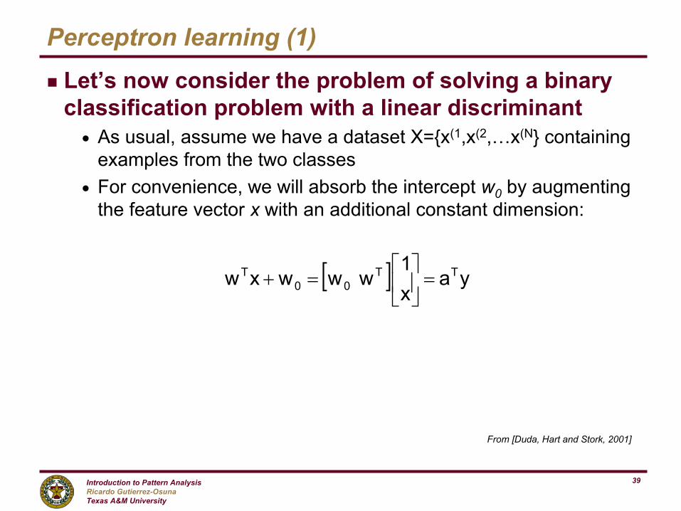
Perceptron learning (1)
g Let’s now consider the problem of solving a binary classification problem with a linear discriminantn As usual, assume we have a dataset X={x(1,x(2,…x(N} containing
examples from the two classesn For convenience, we will absorb the intercept w0 by augmenting
the feature vector x with an additional constant dimension:
[ ] yax1
wwwxw TT00
T =
=+
From [Duda, Hart and Stork, 2001]
Introduction to Pattern AnalysisRicardo Gutierrez-OsunaTexas A&M University
40
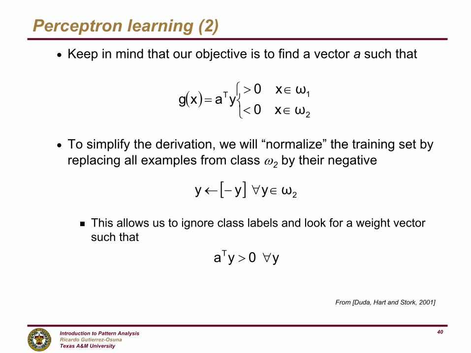
Perceptron learning (2)n Keep in mind that our objective is to find a vector a such that
n To simplify the derivation, we will “normalize” the training set by replacing all examples from class ω2 by their negative
g This allows us to ignore class labels and look for a weight vector such that
y0yaT ∀>
[ ] 2ωyyy ∈∀−←
From [Duda, Hart and Stork, 2001]
( )
∈<∈>
=2
1T
ωx0ωx0
yaxg
Introduction to Pattern AnalysisRicardo Gutierrez-OsunaTexas A&M University
41
Perceptron learning (3)
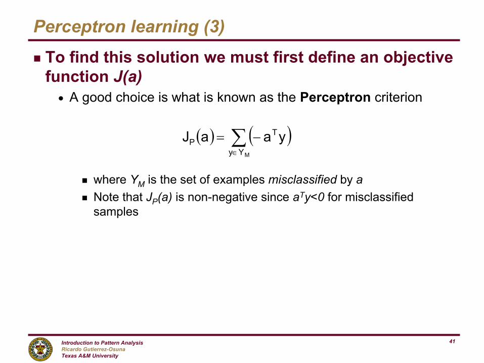
g To find this solution we must first define an objective function J(a)n A good choice is what is known as the Perceptron criterion
g where YM is the set of examples misclassified by ag Note that JP(a) is non-negative since aTy<0 for misclassified
samples
( ) ( )∑∈
−=MΥy
TP yaaJ
Introduction to Pattern AnalysisRicardo Gutierrez-OsunaTexas A&M University
42
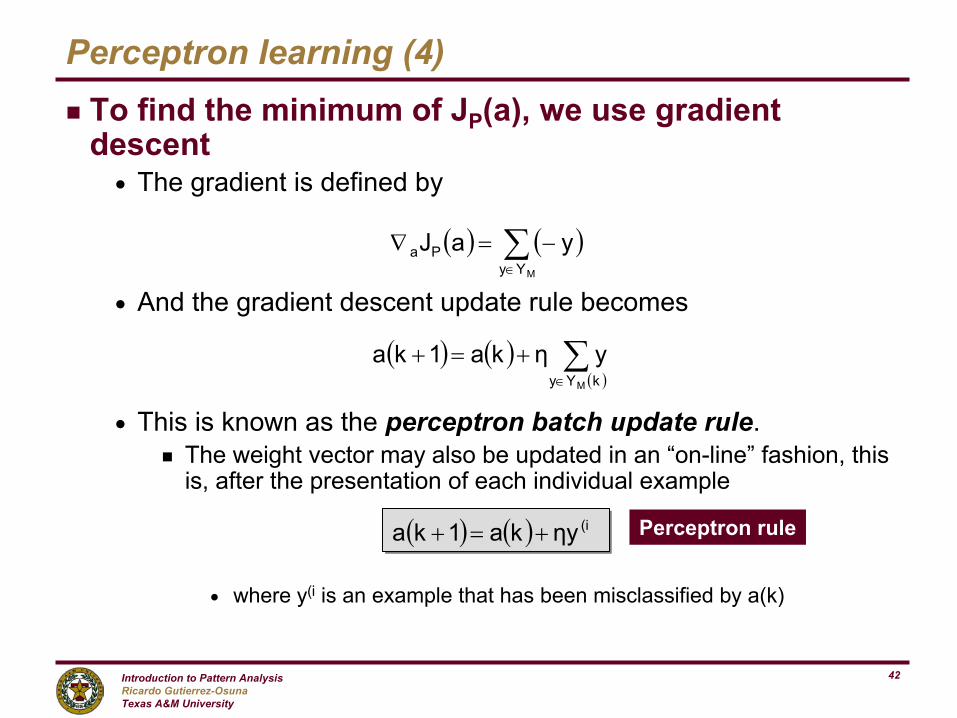
Perceptron learning (4)g To find the minimum of JP(a), we use gradient
descentn The gradient is defined by
n And the gradient descent update rule becomes
n This is known as the perceptron batch update rule. g The weight vector may also be updated in an “on-line” fashion, this
is, after the presentation of each individual example
n where y(i is an example that has been misclassified by a(k)
( ) ( )∑∈
−=∇MΥy
Pa yaJ
( ) ( )( )
∑∈
+=+kΥy M
yηka1ka
( ) ( ) (iηyka1ka +=+ Perceptron rule
Introduction to Pattern AnalysisRicardo Gutierrez-OsunaTexas A&M University
43
Perceptron learning (5)
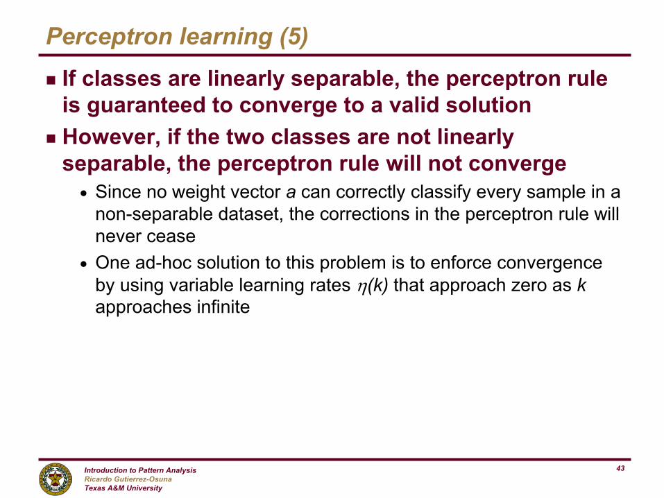
g If classes are linearly separable, the perceptron rule is guaranteed to converge to a valid solution
g However, if the two classes are not linearly separable, the perceptron rule will not convergen Since no weight vector a can correctly classify every sample in a
non-separable dataset, the corrections in the perceptron rule will never cease
n One ad-hoc solution to this problem is to enforce convergence by using variable learning rates η(k) that approach zero as kapproaches infinite
Introduction to Pattern AnalysisRicardo Gutierrez-OsunaTexas A&M University
44
Perceptron learning example
g Consider the following classification problemn class ω1 defined by feature vectors x={[0, 0]T, [0, 1]T}; n class ω2 defined by feature vectors x={[1, 0]T, [1, 1]T}.
g Apply the perceptron algorithm to build a vector ‘a’that separates both classes. n Use learning rate η=1 and a(0) =[1, -1, -1]T.n Update the vector ‘a’ on a per-example basisn Present examples in the order in which they were given above.n Draw a scatterplot of the data, and the separating line you found
with the perceptron rule.
Introduction to Pattern AnalysisRicardo Gutierrez-OsunaTexas A&M University
45
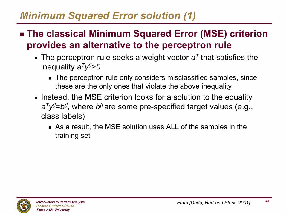
Minimum Squared Error solution (1)
g The classical Minimum Squared Error (MSE) criterion provides an alternative to the perceptron rulen The perceptron rule seeks a weight vector aT that satisfies the
inequality aTy(i>0g The perceptron rule only considers misclassified samples, since
these are the only ones that violate the above inequalityn Instead, the MSE criterion looks for a solution to the equality
aTy(i=b(i, where b(i are some pre-specified target values (e.g., class labels)
g As a result, the MSE solution uses ALL of the samples in the training set
From [Duda, Hart and Stork, 2001]
Introduction to Pattern AnalysisRicardo Gutierrez-OsunaTexas A&M University
46
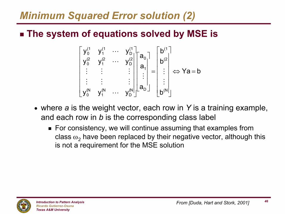
Minimum Squared Error solution (2)
g The system of equations solved by MSE is
n where a is the weight vector, each row in Y is a training example, and each row in b is the corresponding class label
g For consistency, we will continue assuming that examples from class ω2 have been replaced by their negative vector, although this is not a requirement for the MSE solution
bYa
b
bb
a
aa
yyy
yyyyyy
(N
(2
(1
D
1
0
N(D
N(1
N(0
(2D
2(1
2(0
(1D
(11
(10
=⇔
=
M
MM
L
MMM
MMM
L
L
From [Duda, Hart and Stork, 2001]
Introduction to Pattern AnalysisRicardo Gutierrez-OsunaTexas A&M University
47
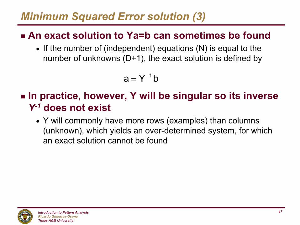
Minimum Squared Error solution (3)
g An exact solution to Ya=b can sometimes be found n If the number of (independent) equations (N) is equal to the
number of unknowns (D+1), the exact solution is defined by
g In practice, however, Y will be singular so its inverse Y-1 does not existn Y will commonly have more rows (examples) than columns
(unknown), which yields an over-determined system, for which an exact solution cannot be found
bYa 1−=
Introduction to Pattern AnalysisRicardo Gutierrez-OsunaTexas A&M University
48
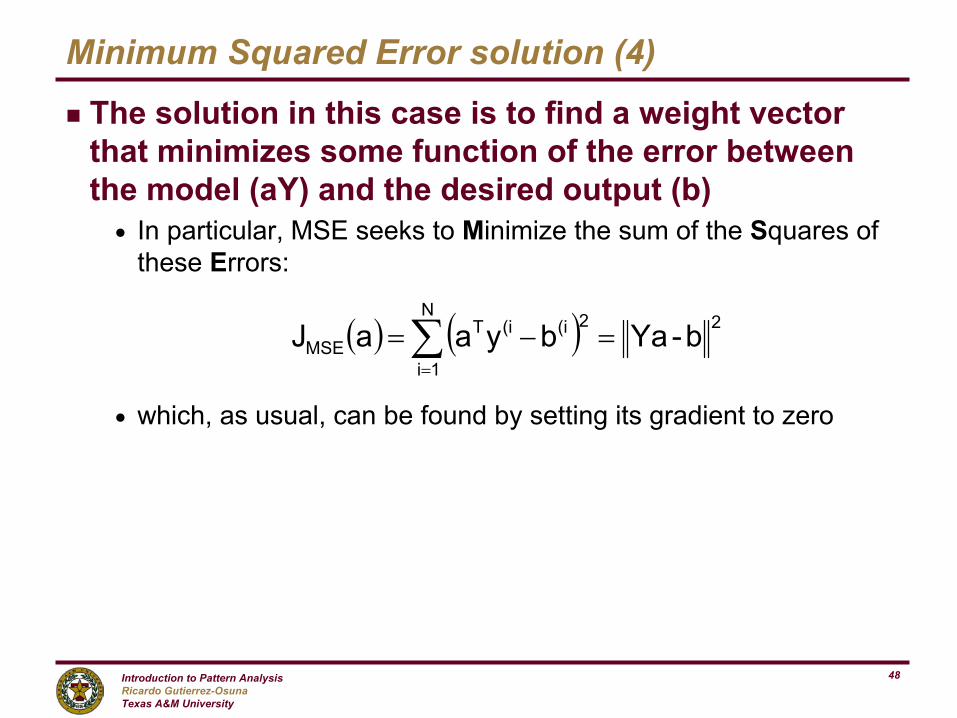
Minimum Squared Error solution (4)
g The solution in this case is to find a weight vector that minimizes some function of the error between the model (aY) and the desired output (b)n In particular, MSE seeks to Minimize the sum of the Squares of
these Errors:
n which, as usual, can be found by setting its gradient to zero
( ) ( ) 2N
1i
2(i(iTMSE b-YabyaaJ =−=∑
=
Introduction to Pattern AnalysisRicardo Gutierrez-OsunaTexas A&M University
49
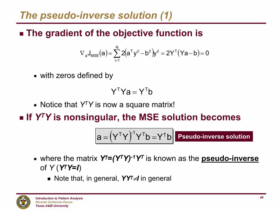
The pseudo-inverse solution (1)
g The gradient of the objective function is
n with zeros defined by
n Notice that YTY is now a square matrix!
g If YTY is nonsingular, the MSE solution becomes
n where the matrix Y†=(YTY)-1YT is known as the pseudo-inverseof Y (Y†Y=I)
g Note that, in general, YY†≠I in general
( ) ( ) ( ) 0bYa2Yybya2aJ TN
1i
(i(i(iTMSEa =−=−=∇ ∑
=
bYYaY TT =
( ) bYbYYYa †T-1T == Pseudo-inverse solution
Introduction to Pattern AnalysisRicardo Gutierrez-OsunaTexas A&M University
50
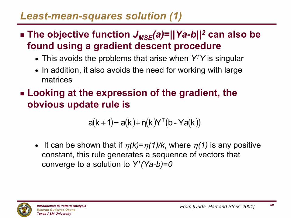
Least-mean-squares solution (1)
g The objective function JMSE(a)=||Ya-b||2 can also be found using a gradient descent proceduren This avoids the problems that arise when YTY is singularn In addition, it also avoids the need for working with large
matrices
g Looking at the expression of the gradient, the obvious update rule is
n It can be shown that if η(k)=η(1)/k, where η(1) is any positive constant, this rule generates a sequence of vectors that converge to a solution to YT(Ya-b)=0
( ) ( ) ( ) ( )( )kYa-bYkηka1ka T+=+
From [Duda, Hart and Stork, 2001]
Introduction to Pattern AnalysisRicardo Gutierrez-OsunaTexas A&M University
51
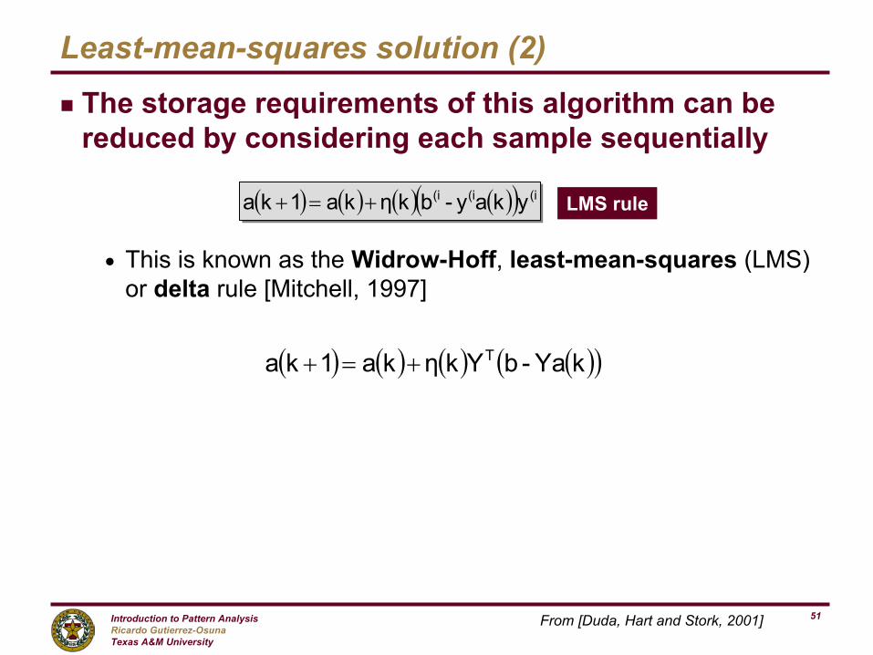
Least-mean-squares solution (2)
g The storage requirements of this algorithm can be reduced by considering each sample sequentially
n This is known as the Widrow-Hoff, least-mean-squares (LMS) or delta rule [Mitchell, 1997]
( ) ( ) ( ) ( )( )kYa-bYkηka1ka T+=+
( ) ( ) ( ) ( )( ) (i(i(i ykay-bkηka1ka +=+ LMS rule
From [Duda, Hart and Stork, 2001]